Improving robustness and reliability of phase-sensitive fMRI analysis using Temporal Off-resonance Alignment of Single-echo Timeseries (TOAST)

Abstract

Echo Planar Imaging (EPI), often utilized in functional MRI (fMRI) experiments, is well known for its vulnerability to inconsistencies in the static magnetic field (B₀). Correction for these field inhomogeneities usually involves measuring the magnetic field at a single time point, and using this static information to correct a series of images collected over the course of one or multiple experiments. However, common phenomena, such as respiration and motion, change the characteristics of the B₀ field homogeneity in a time-dependent and often unpredictable manner, rendering previous field measurements invalid. The effects of these changes are particularly large in the image phase, due to its direct and sensitive relationship to the magnetic field, and methods utilizing complex information can suffer enormously. This dependence can be exploited to estimate the temporal dynamics of the B₀ field. Use of this information to correct fMRI data can provide more effective motion correction, reduce temporal “noise,” and can substantially restore statistically significant power to complex fMRI data analysis. All of the necessary information is embedded in complex EPI images, and results indicate this is a robust way to improve the quality of fMRI data, especially when used with complex analysis.

Introduction

Experiments in functional MRI (fMRI) often involve single-shot gradient echo echo-planar imaging (GE-EPI) pulse sequences to maximize acquisition speed and blood oxygenation level dependent (BOLD) contrast (Ogawa et al. 1990). However, inhomogeneities in the static magnetic field can result in severe artifacts, most notably image warping and signal loss. Correcting these errors has been a consistent field of research. In general, this correction is a two-step process, involving estimation of the spatially dependent main field offsets followed by image correction based on the estimated map. The field map can be calculated in a variety of ways (Jezzard and Balaban, 1995; Reber et al., 1998; Kannengiesser et al., 1999), often with two or more reference images acquired at different echo time (TE) values (Jezzard and Balaban, 1995). In practice, the field offsets are assumed to be temporally invariant, justifying the correction of an entire time series of images with a single map. Although large scale inhomogeneities are generally constant over experimental time series, this assumption fails when considering sensitive phase data due to the small scale changes associated with the resonance offset caused by the breathing cycle (Van de Moortele et al., 2002; Barry and Menon, 2005) and slight changes in the orientation of tissue boundaries. The former is unavoidable in vivo, and subject movement, whether inside or outside the field of view, can cause non-negligible changes in the magnetic field due to reorientation of the aforementioned susceptibility profile. When the field changes, so does the induced warping, which can have significant consequences. For example, this warping and its associated voxel intensity modulation can cause less reliable bulk motion correction (Jezzard and Clare, 1999). In addition, spatial specificity is sacrificed as the point spread function associated with the off-resonance changes (Robson et al., 1997). These phenomena are well known and often have non-negligible effects, most notably additional temporal (non-white) “noise” that reduces strength and specificity of activation statistics. Accompanying phase changes can have similar detrimental impact on complex, or phase sensitive activation models (Menon, 2002; Rowe and Logan, 2004). In depth performance analysis of these methods and identification of their sensitivity to these potentially large phase variations has resulted in the recognition of the potential value of correcting for off-resonance dynamics (Nencka and Rowe, 2007). An alternative method involves a model for magnitude activation in complex data, and has been developed to account for phase variations (Rowe, 2005). However, it can be difficult to provide valid regressors for phase, and even when properly modeled, dynamic image warping artifacts still remain, currently making this a less attractive solution.

Current methods to combat the problem of temporal field variations include low resolution field mapping with a type of dual-echo single-shot EPI (Roopchansingh et al., 2003), zero-order field offset correction using only a pair of navigator echoes (Jesmanowicz et al., 1993; Van de Moortele et al., 2002), and real-time magnetic field shimming based on a priori knowledge of the field changes resulting from a regular phenomena (Van Gelderen et al., 2007). While each of these provides certain benefits, issues exist preventing their widespread use. Each method struggles to provide field maps with a combination of high resolution, SNR and spatial order to be useful to correct for commonly unpredictable and nonlinear temporal field dynamics. Alternatively, effects from certain field variations may be removable without either field measurements or shimming by monitoring physiologic phenomena that influence field changes, such as breathing rate. Signal components at the measured frequencies can then be retrospectively accounted for (Hu et al., 1995). This method not only requires the acquisition of physiologic information but may remove signal of interest aliased to the frequency of the physiologic fluctuations while failing to remove “noise” due to field changes arising from unmonitored sources.

One of the most common methods of field map estimation involves acquiring images at different echo times and comparing the difference in phase evolution between the two (Jezzard and Balaban, 1995). Given two images I₁ and I₂, with echo times TE₁ and TE ₂ respectively, the general equation for the estimated resonance offset in a voxel at location (m,n), denoted by Δω̑ (m,n) (radians/sec), can be written as

$$\mathrm{\Delta }\stackrel{⌢}{\omega }(m,n)=\frac{arg(I_2(m,n)I_1^{\ast }(m,n))}{({TE}_2-{TE}_1)}$$ (1.1)

where I_i (m, n) represents the complex value of the voxel with coordinates (m,n) in image i, * denotes complex conjugation, and the arg operator returns the phase angle of its argument. The SNR of Δω̑(m,n) is proportional to the ratio of TE₂ − TE₁ (referred to as ΔTE) divided by the geometric mean of the standard deviation of the phase noise in the two images. Thus, increasing the difference in echo times decreases variation in the field map, but with such an increase, complicated phase wrapping can occur, along with an offsetting increase in phase variance resulting from the longer TE. These issues require the echo time difference be kept relatively short and multiple references are sometimes acquired to achieve the necessary accuracy (Reber et al., 1998), inherently requiring more time. For these reasons, it is not surprising that previous evaluation of methods based on Equation (1.1) for dynamic field mapping has not produced promising results (Hutton et al., 2002).

The recent method of Lamberton et al. (2007), which also utilizes Equation (1.1) has been described which utilizes the assumption of invariance of the RF pulse phase (and thus the initial spin phase, Φ₀) from shot to shot to alleviate the need for two unique images at each time point to calculate the corresponding field map. Rather, because Φ₀ is the same for all images, it can be used for reference (as I₁ is in Equation (1.1)) as the image phase at TE = 0. Additionally, this method provides a maximum ΔTE without increasing the echo time of each acquired image. However, because the static field will likely cause the phase of each image to wrap many times over the course of TE, complicated phase unwrapping procedures are necessary to find the correct phase accumulation in reference to the initial phase. In order to apply the method, an initial measurement of Φ₀ is also required before acquiring the image time series.

The method of Lamberton et al. (2007) can be extended to find the difference, δω̑, between the resonance offset during acquisition of the t^th image, Δω_t, and the average resonance offset during the entire series acquisition, $\overline{\mathrm{\Delta }\omega }$, rather than attempting to directly calculate the absolute resonance offset at each time point. Further analysis yields

$$\delta {\stackrel{⌢}{\omega }}_t(m,n)=\frac{arg\left\{I_t(m,n){\displaystyle \sum _{j=1}^N}\frac{I_j^{\ast }(m,n)}{\mid I_j(m,n)\mid }\right\}}{TE}$$ (1.2)

for a series of N images with identical TE. This provides two significant advantages over the method as presented by Lamberton et al. (2007). First, while ΔTE remains TE, the phase of I_t will not normally differ by >2π from the average image phase (represented by the summation in Equation (1.2)), which removes the need for any phase unwrapping. Second, correction for temporal variations in off-resonance (using the δω̑_t measurements) can be performed without any reference at all, as δω̑_t does not depend on Φ₀. While a static effect would remain in this case, a single measurement of Δω (similarly to Lamberton et al. (2007)) provides the means to fully correct every image in a series with no need to apply any phase unwrapping. The benefit of the proposed method is mostly realized through the convenience of avoiding phase unwrapping and the ability to correct for field dynamics in the absence of any reference. Performance of the methods, determined by the accuracy of the measured fields, should be very similar, except when phase is incorrectly unwrapped, as both otherwise share similar sources of error.

Theory

The proposed method relies on the assumption that the initial spin phase, Φ₀, remains constant throughout the acquisition of a series of images, although the value of Φ₀ is inconsequential. The validity of this assumption is a significant topic of Lamberton et al. (2007), and is well addressed in the literature. It is also true that, in general, any multi-shot imaging modality requires RF pulse consistency from shot to shot and as a result, Φ₀ is almost always necessarily assumed to be constant through time. Other field mapping methods making this assumption are commonly used with a great degree of success (Reber et al., 1998; Zeng et al., 2004), further illustrating its practical validity.

Let the value of Φ₀ represents the phase of an image, I₀, acquired with TE = 0. In other words, Φ₀ (m, n) = arg(I₀ (m, n)), where I₀ (m, n) is the complex value of the voxel with coordinates (m,n). The value of Φ₀ is assumed to be unknown, but constant from acquisition to acquisition in a series of N images, with each image in the series having echo time TE. Then from Eq. (1.1), the estimated magnetic field offset in the voxel with coordinates (m,n) in the t^th image, represented as Δω̑_t (m, n) (radians/sec) can be written as

$$\mathrm{\Delta }{\stackrel{⌢}{\omega }}_t(m,n)=\frac{arg(I_t(m,n)I_0^{\ast }(m,n))}{TE}.$$ (2.1)

The average estimated magnetic field offset present during the entire series acquisition in the voxel with coordinates (m,n), represented as $\overline{\mathrm{\Delta }\stackrel{⌢}{\omega }(m,n)}$, (in radians/sec) can be similarly written as

$$\overline{\mathrm{\Delta }\stackrel{⌢}{\omega }(m,n)}=\frac{arg(\overline{I(m,n)}{I}_0^{\ast }(m,n))}{TE}$$ (2.2)

$$\overline{I(m,n)}=\sum _{j=1}^N\frac{I_j(m,n)}{\mid I_j(m,n)\mid }.$$ (2.3)

Given the unknown nature of I₀, neither Eq. (2.1) nor Eq. (2.2) can be calculated directly. However, by writing Δω̑_t (m, n) in terms of $\overline{\mathrm{\Delta }\stackrel{⌢}{\omega }(m,n)}$ plus some offset, δω̑_t (m, n),

$$\mathrm{\Delta }\stackrel{⌢}{\omega }(m,n)=\overline{\mathrm{\Delta }\stackrel{⌢}{\omega }(m,n)}+\delta {\stackrel{⌢}{\omega }}_t(m,n)$$ (2.4)

it is possible to solve for δω̑_t (m, n) by combining Eqns. (2.1–2.4), and rearranging the variables to arrive at Eq. (1.2), which does not directly depend on I₀ (m, n).

Materials and Methods

Simulation

A computer simulation was designed in Matlab (The Mathworks, Natick, MA, USA) to test the potential benefits of the time varying magnetic field correction on an fMRI series. First, gradient waveforms were generated for the given imaging parameters (GE-EPI, 96×96 matrix, TE = 42.7 ms, BW = 125 kHz, echo spacing = 0.708 ms, FOV = 24 cm). Maps of spin density, transverse relaxation time and main magnetic field offset, denoted as ρ(x, y), $T_2^{\ast }(x,y)$ and ΔB₀ (x, y) respectively, were provided as input, and the k-space signal based on these three input maps and the generated gradient waveforms, G_x and G_y, was output according to

$$S(m\mathrm{\Delta }t)=\sum _{q=-N_x/2}^{N_x/2-1}\sum _{r=-N_y/2}^{N_y/2-1}\rho (q\mathrm{\Delta }x,r\mathrm{\Delta }y)e^{\left(-\frac{m\mathrm{\Delta }t}{T_2^{\ast }(q\mathrm{\Delta }x,r\mathrm{\Delta }y)}\right)}{e}^{i\gamma \left(\sum _{w=0}^m(G_x(w\mathrm{\Delta }t)q\mathrm{\Delta }x+G_y(w\mathrm{\Delta }t)r\mathrm{\Delta }y)+\mathrm{\Delta }{B}_0(q\mathrm{\Delta }x,r\mathrm{\Delta }y)\right)}.$$ (3.1)

where N_x and N_y are the number of discrete points in ρ along the x and y dimensions. After acquisition of S, the samples are placed accordingly in the 2D k-space matrix for image reconstruction. In Eq. (3.1), Δt is not necessarily the sampling interval, but is the resolution with which the summation in the exponential is computed. The values of m at which samples are actually recorded are not necessarily sequential, and will be determined by the gradient sequence and other parameters. As Δx, Δy and Δt approach zero, the summations become better estimations of the integral representing the theoretical signal, but computation time grows quickly. With larger values, some error is induced through inability to properly account for k-space truncation and poorer modeling of the continuous image acquisition process.

Two different series of 276 images were created in this way using the same, temporally constant, ρ(x, y) map for each series. In each series, identical magnitude and/or phase “activations” were simulated by locally modulating the value of $T_2^{\ast }$ for magnitude change and ΔB₀ for phase change in a block design pattern (20 repetitions rest followed by 16 epochs of 8 repetitions active and 8 repetitions rest). Six different combinations of activation types and sizes were considered, indicated by pairs of $T_2^{\ast }$ and ΔB₀ changes in the first two columns of Table 1. Each combination was simulated in 6 different 3 voxel by 3 voxel regions, shown in Fig. 1(a). The use of the various locations is directed at averaging out the influence of differences in spatial contrast, size of field variations, and field gradients in the field offset.

Table 1.

Simulation parameters and results

$\mathrm{\Delta }{\text{T}}_{2-}^{\ast }$ (ms)	ΔB0 (nT)	CNR1,2	ΔΦ (°)	Series A (control)						Series B, static correction						Series B, dynamic correction
				z-statistics1		${\beta }_0^1$	β11 × 107	${\beta }_2^1\times {10}^2$	σ1 × 102	z-statistics1		${\beta }_0^1$	${\beta }_1^1\times {10}^7$	${\beta }_2^1\times {10}^2$	σ1 × 102	z-statistics1		${\beta }_0^1$	${\beta }_1^1\times {10}^7$	${\beta }_2^1\times {10}^2$	σ1 × 102
				MO	CP					MO	CP					MO	CP
.432	0	1.24	0	4.09	4.12	.408	.49	2.68	1.08	3.71	1.18	.406	−4.56	2.58	1.15	3.91	3.66	.410	4.77	2.72	1.14
.216	9.17	.49	6	1.61	.941	.407	−1.88	1.06	1.08	1.64	.70	.405	−4.36	1.10	1.15	1.62	1.04	.408	4.92	1.14	1.14
.432	4.58	1.19	3	3.90	3.27	.408	1.99	2.56	1.08	3.63	1.14	.406	−4.70	2.51	1.15	3.73	3.11	.409	4.92	2.62	1.14
0	4.58	.07	3	−.25	−.24	.406	.84	−.15	1.08	−.16	.38	.404	−4.29	−.14	1.15	−.14	−.12	.407	4.88	−.09	1.14
.432	9.17	1.01	6	3.59	2.19	.408	−.67	2.38	1.08	3.48	1.06	.406	−4.35	2.41	1.15	3.50	2.29	.409	4.76	2.47	1.14
.216	4.58	.56	3	1.83	1.52	.407	−.92	1.20	1.08	1.75	.76	.405	−4.48	1.19	1.15	1.79	1.49	.408	4.92	1.25	1.14

¹Average value over all regions of interest.

²CNR = β₂/(2*σ).

Figure 1.

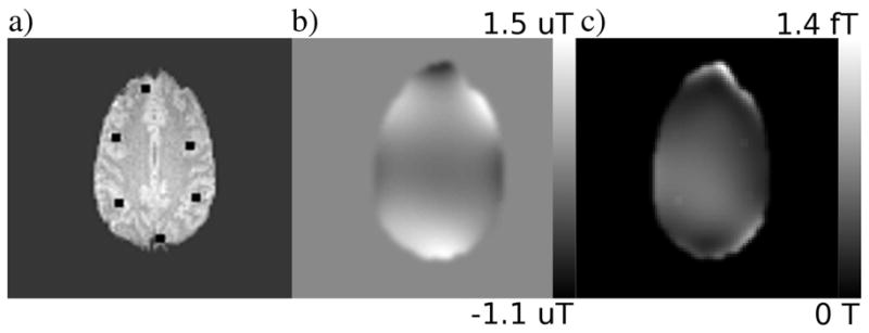
Spin density map, ρ, used for simulation (a). Regions of simulated activation are represented by black squares. The global, static field offset applied in simulation and the variance of the simulated dynamic field used in simulation are shown in b and c, respectively.

The first of the two series (series A) was simulated under the influence of an additional global, static, ΔB₀ field, which is shown in Fig. 1(b). The second series (series B) was simulated under the influence of a global, time variant, δB₀ field in addition to the aforementioned static field, so that the total field present was ΔB₀ + δB₀. The variance of the time variant field is shown in Fig. 1(c). All fields used for simulation were taken from fields modeled directly from experimental data of a human subject performing a deep breathing task at 0.167 Hz. The initial value of the δB₀ map for series B was equal to zero so that the initial field offset was identical for series A and B and equal to ΔB₀. In order to measure this initial field inhomogeniety, an additional 10 images were simulated using this initial ΔB₀ time point only, and images 2, 4, 6, 8 and 10 had the TE increased to 47.2 ms.

The only difference between series A and series B is the time varying portion of the magnetic field offset. As such, series A serves as a control, allowing for determination of the effect of the time varying field as well as the quality of the correction.

Series A was corrected for static field inhomogeneities using an initial measurement of the field offset, Δω̑₁, acquired with the first 5 pairs of simulated images using Eq. (1.1). Series B was corrected two different ways, first identically to the static correction for series A, and secondly using a dynamic field correction, using maps of δω̑_i calculated with Eq. (3.1). Subsequently, Δω̑_i was calculated for images 11 through 286 (the first 10 images were discarded after being used to find Δω̑₁ as described above), and a fourth order polynomial was fit to each Δω̑_i map, helping to eliminate spatially varying random noise. Additionally, this process prevented the removal of the local high spatial frequency ΔB₀ modulations so that phase activations remained in the corrected time series. As a final processing step, the polynomial field models were allowed to smoothly fall to zero outside the object area by applying a mask over the imaged object, which had been previously dilated and smoothed by a Gaussian filter with FHWM of 4 voxels.

Once magnetic field estimations had been made using the proposed method, the appropriate corrections were applied using the Simulated Phase Rewinding (SPHERE) method (Kadah and Hu, 1997). In the static case, the initial Δω̑₁ map was applied to each image, while the Δω̑_i map was used to correct the i^th image in the dynamic case. This provided a direct means to evaluate the effects of dynamic correction.

Activation statistics were calculated for each corrected time series using two different methods. The first method, most typically used, analyzes only the magnitude of the image time series, and is thus termed the magnitude-only (MO) method (Bandettini et al., 1993; Rowe and Logan, 2005). This was implemented with a general linear model (GLM) with regression for constant and linear trends, as well as for the task reference function, which was equal to 1 during stimulus and −1 during rest. The second method used was the complex constant phase (CP) method (Rowe and Logan, 2004). This technique has been shown to bias against voxels containing phase changes, useful due to their likely association with venous macrovasculature (Menon, 2002; Nencka and Rowe, 2007). Comparisons between the activation statistics (z-statistics) from the different time series were made in order to gain insight into (i) how temporal variations in ΔB₀ affect the activation statistics, and (ii) the effectiveness of the dynamic field calculation (and subsequent correction) method in restoring the original activation.

Phantom

A spherical phantom filled with SiO₂ oil was imaged to evaluate the potential of the proposed dynamic field mapping method to correct for the effects of a time varying magnetic field offset in a controlled environment. The experiment was performed using a GE Signa LX 3T scanner (General Electric, Milwaukee, WI) with a GE-EPI pulse sequence (8 axial slices, 64×64 matrix, TE = 44.1 ms, TR = 1 s, flip angle = 45°, BW = 125 kHz, echo spacing = 0.624 ms, FOV = 24 cm, slice thickness = 3.8 mm, 276 repetitions). During the acquisition of the images, perturbations in the main field were induced by manually moving a bottle filled with water along Inferior-Superior axis at a rate of 0.2 Hz. These field perturbations would mimic those seen with motion outside of the field of view, such as breathing. This is in contrast to motion within the field of view, which would also cause field changes, but is not simulated here. The perturbation frequency of 0.2 Hz was chosen to estimate the breathing rate, but perturbation rate should not affect the results, as long as intra-acquisition effects remain small. The peak-to-peak displacement of the bottle was approximately 20 cm, and it was brought as close to the phantom as possible without entering the field of view.

In this case, no initial reference of an absolute field offset map was calculated, i.e. only the maps of δω̑_i were estimated and applied, as correction for δω̑_i alone should reduce effects of the temporal variations in Δω.

The raw estimated maps were processed in an identical fashion to that described in the simulation methods and the SPHERE method of correction was used as well.

Human

Two separate experiments were performed with a human subject to evaluate the dynamic field map corrections in vivo in two different situations where temporal changes in the magnetic field were likely to occur. Experiments were both performed using the same GE 3T scanner as for the phantom experiment. A GE-EPI pulse sequence was used for both experiments (9 axial slices, 96×96 matrix, TE = 42.8 ms, TR = 1 s, flip angle = 45°, BW = 125 kHz, echo spacing = 0.768 ms, FOV = 24 cm, slice thickness = 2.5 mm, 296 repetitions). Even repetitions up to repetition 20 had an increased TE of 47.8 ms and were used in Eq. (1.1) for calculation of Δω̑₁. The first 20 repetitions were subsequently discarded, leaving the last 276 repetitions for further analysis. Smaller voxel size (and thus longer TE) was used to increase the effect of the field variations, which are smaller in these experiments than in the phantom.

Each experiment involved a combination of two tasks. The task common to both was visually cued bilateral finger tapping (the “functional” task), which followed a simple block design (20 s off, 16 epochs of 8 s on, 8 s off, for 0.0625 Hz task on/off frequency, starting at repetition 21). In the first experiment, the second task was deep, heavy breathing at a rate of 0.167 Hz. The second experiment replaced the heavy breathing with opening and closing of the jaw at the same rate. In each case, the timing of the second task was cued visually along with the “functional” task cue. The purpose of the second, “field modulating” task, was to modulate the main field at a known rate in order to make the effects on the time series clear and to allow more straightforward evaluation of the correction.

The experimental design provides an initial estimate of the field offset, Δω̑₁, and thus, both static and dynamic correction were performed in the same manner as described for the simulation. Again, the SPHERE method was used to apply the correction.

Following the correction for the magnetic field offset, each corrected image series was motion corrected using the AFNI (Cox, 1996) 3dvolreg program. Motion correction was applied to the magnitude images only, as is usually the case. Available motion correction techniques are not optimized for complex valued data and are thus not applied. The evaluation of such techniques, although necessary, is beyond the scope of this manuscript.

The processing resulted in four time series for each experiment: static field corrected with and without motion correction; dynamic field corrected with and without motion correction. Activation statistics using both the MO and CP methods were computed in the same manner as described for the simulation, only in this case, the first 10 images were discarded to allow the magnetization to reach steady state and the task reference function was delayed 4 seconds to account for hemodynamic delay. Because motion correction was applied only to magnitude data, complex activation statistics were not calculated after applying the motion correction.

Results

Simulation

In order to analyze the effects of the time varying magnetic field as well as the quality of the correction method, 100 iterations of each image series were processed, each with the addition of random, normally distributed noise added to both the real and imaginary channels of the simulated k-space signal. The amplitude of the added noise was such that the maximum contrast to noise ratio in the magnitude signal was approximately 1. Because six different combinations of magnitude and or phase activations were used, a total of 600 iterations of each series were performed, with 100 iterations for each of the different activation sizes in each region.

The statistics generated for Figure 2 originate from images simulated with a unique activation type from Table 1 in each region (iterated 100 times). The top left ROI (Fig. 1(a)) contains the combination from the first row of Table 1 (no ΔB₀ change) and the regions were assigned the remaining combinations, down the rows of Table 1, in clockwise order. The mean values (z-statistics, beta coefficients) are computed from 100 samples, and the power being referred to is the percentage of times a voxel was active above a p = 0.01 unadjusted threshold.

Figure 2.

fMRI statistics resulting from simulated activation. z-statistic maps shown with an unadjusted threshold of p < 0.01. All power maps shown with threshold of power ≥ 5%. Rows labeled a–h.

The nearly total lack of voxels with a mean CP z-statistic above threshold (Fig. 2(d)) as well an almost complete loss of power (Fig. 2(f)) after static correction alone is precisely the expected result in the presence of the time variant field. Additionally, the losses appear nearly completely recoverable after dynamic correction. The observed detrimental effects, which are not accounted for by the static correction, can be attributed to phase changes caused by the variable field, which are greatly reduced by the dynamic corrections. Such variations will result in abnormally high complex residuals, reducing statistical significance in voxels that have no true physiologically related phase changes. Dynamic warping and shifting in the image from field variations can be visualized through the regression beta coefficients of the static images (Figs. 2(g) and (h)). The regression attempts to model the signal changes due to these effects, which are most apparent from elevated beta coefficients in areas of high spatial contrast, such as the object boundaries. Again, these undesirable signal components are largely diminished after dynamic correction.

The effect on MO activations and power (Figs 2(a) through (c)) is not as clear, but comparison of the two correction methods against the control suggests that the field variations reduce the precision and accuracy of the calculated activations, with evidence provided in Fig. 3 and Fig. 4. The data displayed in these figures, as well as that used in the following analysis, comes only from voxels within the six ROIs after expanding the regions by 2 voxels on each side. The apparent tighter clustering of points around a 45° line in Fig. 3 and narrower error distributions in Fig. 4 with correction suggest that the statistics tend more often toward the control (expected) value than without. To confirm this, concordance correlation coefficients (Lin, 1989) between the control and both the static and dynamic mean MO activation z-statistics were computed to determine the reproducibility of the true (control) activations in each, resulting in values of 0.902 (Z = 1.485, p = 0.069) and 0.919 (Z = 1.58, p = 0.057) respectively. High coefficients (low p-values) suggest the presence of a one-to-one relationship between data sets, in contrast to the Pearson correlation coefficient, which detects any linear relationship. These results provide evidence for better reproducibility in dynamically corrected images. Additionally, the variance of the mean MO z-statistic error (from the control) in the static and dynamic results were ${\stackrel{⌢}{\sigma }}_{\mathit{stat}}^2=0.623$ and ${\stackrel{⌢}{\sigma }}_{\mathit{dyn}}^2=0.512$ respectively, with a hypothesis test of ${\text{H}}_0:{\sigma }_{\mathit{stat}}^2\le {\sigma }_{\mathit{dyn}}^2$ vs. ${\text{H}}_{\text{a}}:{\sigma }_{\mathit{stat}}^2>{\sigma }_{\mathit{dyn}}^2$ resulting in p = 0.0018 (F(899, 899) = 1.215). Additionally, the variances of the error in the power are ${\stackrel{⌢}{\sigma }}_{\mathit{stat}}^2=199.74$ and ${\stackrel{⌢}{\sigma }}_{\mathit{dyn}}^2=174.91$, and the same test results in p = .0233 (F(899, 899) = 1.142). It is also important to note that t-tests for non-zero mean of the error in all of these cases is not significant. This evidence strongly suggests that 1) on average, MO statistics in dynamically corrected data will have less variation about the true value, and 2) with correction, the probability that voxels will be above the threshold chosen here will be closer to the probability of being above threshold in the absence of any changing field.

Figure 3.

Scatter plots of mean MO z-statistics for static correction vs. control (a) and dynamic correction vs. control (b). Also shown, a scatter plot of mean CP z-statistics for the dynamic correction vs. control (c). Points are color coded by the amount of variation of the dependent variable from the control (small variation = dark blue, large variation = red).

Figure 4.

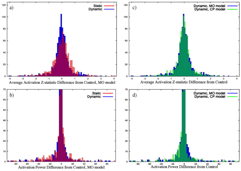
Histograms of static and dynamic mean MO Z-statistic error, defined as difference from control (a), static and dynamic MO power error (b), MO and CP Z-statistic error after dynamic correction (c), and MO and CP power error after dynamic correction (d). Voxels were included in the analysis in contained by regions defined by expanding the active ROIs (see Fig. 1(a)) by 2 voxels on each side.

Similar comparison can be made between the two statistical models with dynamic correction. The dynamic and control mean CP z-statistics have a concordance correlation coefficient of 0.911 (Z = 1.53, p = 0.063), indicating reproducibility similar to that of the MO statistics. A test of ${\text{H}}_0:{\sigma }_{\mathit{dyn},MO}^2\le {\sigma }_{\mathit{dyn},CP}^2$ vs. ${\text{H}}_{\text{a}}:{\sigma }_{\mathit{dyn},MO}^2>{\sigma }_{\mathit{dyn},CP}^2$, where ${\sigma }_{\mathit{dyn},CP}^2$ and ${\sigma }_{\mathit{dyn},MO}^2$ represent the CP and MO power error variances, does not provide a significant result ( ${\stackrel{⌢}{\sigma }}_{\mathit{dyn},MO}^2=174.91,{\stackrel{⌢}{\sigma }}_{\mathit{dyn},CP}^2=165.00$, F(899, 899) = 1.06, p = 0.193). However, the same test with ${\sigma }_{\mathit{dyn},CP}^2$ and ${\sigma }_{\mathit{dyn},MO}^2$ equal to the mean CP and MO z-statistic error variances respectively, results in p<0.005 ( ${\stackrel{⌢}{\sigma }}_{\mathit{dyn},MO}^2=0.512,{\stackrel{⌢}{\sigma }}_{\mathit{dyn},CP}^2=0.390$, F(899, 899) = 1.312), providing evidence supporting a reduction in statistical error variation across voxels for the CP model when used in conjunction with the dynamic correction.

The validity of previous analysis using the F-test for difference in variance between populations relies on normally distributed and independent populations. The distributions in Fig. 4 appear normally distributed and correlations between populations were moderate (r < 0.45) in all cases, with the exception of the final test between the mean CP and MO z-statistic error variances after dynamic correction (r = 0.975). Correlation between populations will reduce the significance of these tests, however the large sample sizes used will diminish the effect. To appropriately qualify the significance of the results, the null distribution of the random variables was verified for every test case by Monte Carlo simulation (10,000 iterations).

Phantom

The variance of the induced field perturbations is shown in Figure 5(a). The effect these magnetic field dynamics have on the series of phantom images can be visualized well through the voxel power spectra. Fig. 6 displays the power spectrum of the magnitude signal from a particularly affected voxel, emphasizing the large component at approximately 0.2 Hz corresponding to the frequency of the field perturbations. The voxel-wise amplitude of the power spectrum at 0.2 Hz (Figs. 7(a) and (b)) gives a good indication of the effect of the time varying field in both the magnitude and the phase through time. Two important things are made clear by these images. First, the most affected voxels in the magnitude power spectra occur in areas of high spatial contrast along the phase encoding direction (top to bottom), as expected. Second, the stronger amplitude in the power spectra near the bottom of the image reveals the origination of the applied field perturbations.

Figure 5.

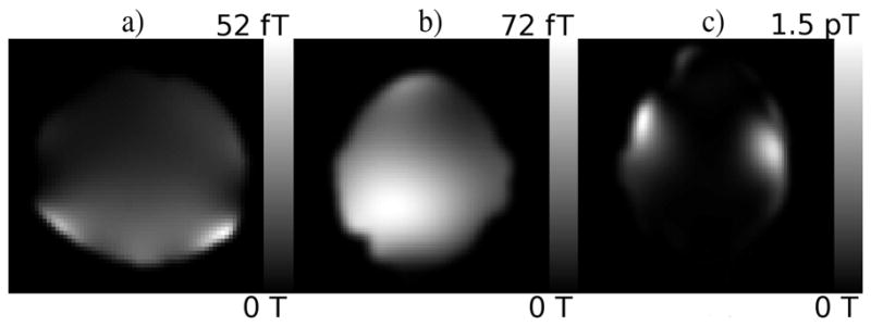
Maps of the temporal variance in the estimated magnetic field during the phantom, human with heavy breathing, and human with jaw motion experiments are shown in a, b and c respectively.

Figure 6.

Power spectra of a single voxel time series with and without correction. The same plot is shown full scale (a) and at reduced scale (b).

Figure 7.

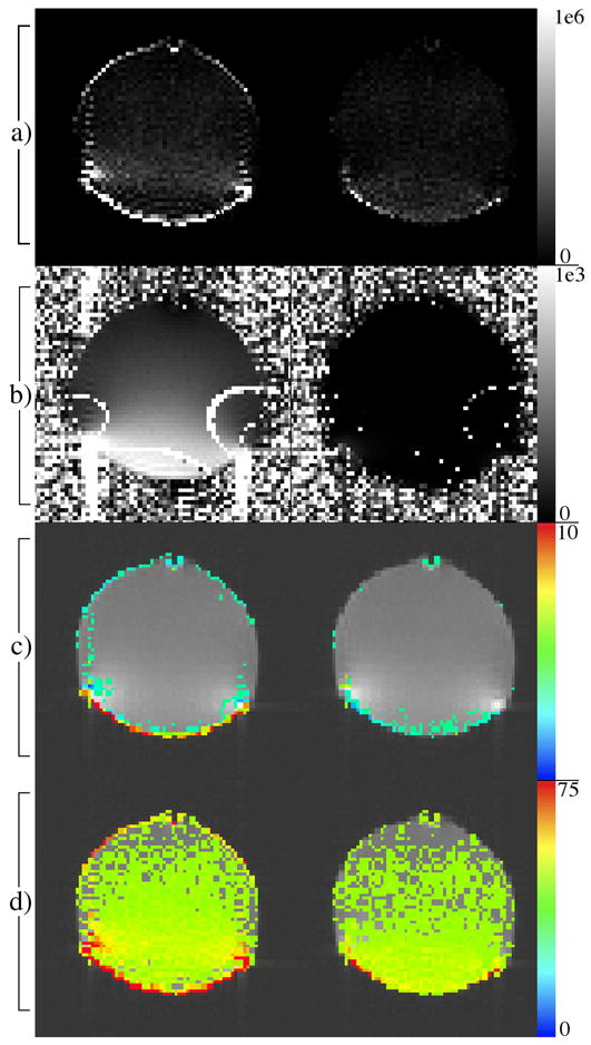
Voxel-wise maps shown are amplitudes of the magnitude (row a) and phase (row b) power spectra at 0.2 Hz, regression coefficients of a 0.2 Hz sine wave (row c) and mean squared error of a regression fit of a constant and linear reference (row d). Row c and row d shown with threshold of 2 and 17.5 respectively. Images on the right and left correspond to data with and without dynamic correction respectively.

Further evidence of the effect of the temporal field perturbations is provided through two regression analyses. The first fit a 0.2 Hz sinusoid, including regressors for a constant and linear trend. The sinusoid phase was determined by the 0.2 Hz component in the image phase time course. The sinusoid regression coefficients (Fig. 7(c)), whose values indicate the effect of the field variations on the voxel magnitude, are largest in areas of high spatial contrast, in agreement with the previous data. In the second regression the sinusoid reference was removed and the variance of the residuals (shown in Fig. 7(d)) was used as the indicator of the size of the effect of the changing field, with larger residuals implying larger effect. These results are consistent with the previous evidence.

The desired consequence of the dynamic correction is reduced signal characteristics correlating with applied field perturbations while maintaining a similar level of noise. This is demonstrated by reduction of the large 0.2 Hz peak in the power spectrum (Fig. 6, Fig. 7(a) and (b)), and Fig. 6 shows reduction in several smaller structural components, while the noise floor appears consistent. The results of the regression analyses are similar. Specifically, Fig. 7(d) further suggests that no additional signal is induced by the correction, which would increase the residuals shown here.

Human

The temporal variance in the estimated magnetic field is shown for the heavy breathing and jaw motion experiments in Figures 5(b) and (c). The activation z-statistic maps computed for both the MO and CP models (Fig. 8) show recovery of CP activation statistics after correcting for the dynamic field as suggested by simulation. At a false discovery rate (FDR) corrected threshold for multiple comparisons (Logan and Rowe, 2004) of p < 0.05, practically all of the complex activation is eliminated in the static case for both experiments. Also corroborating simulated results, dynamic correction has a less obvious impact on the MO activations. Activation maps (not shown) resulting from the same finger-tapping task with no intentional field perturbations showed similar results, although the change in the complex activation was not quite as dramatic. Although the correction appears to provide little at the provided threshold in this case, further analyses gives evidence for a benefit of dynamic correction in the magnitude of the image time series which could lead to more significantly improved activation statistics for tasks with less robust active response or requiring motion nearer to the imaging field of view.

Figure 8.

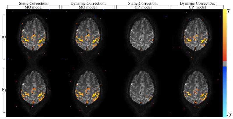
Activation maps (z-statistic) corresponding to a finger tapping task in a single slice in experiments where the subject was asked to additionally breath heavily at 0.167 Hz (row a) or open and close their mouth at 0.167 Hz (row b). Voxels were considered active at a FDR corrected threshold of p < 0.05.

The power in the magnitude signal at 0.167 Hz (Fig. 9) illustrates how the dynamic correction reduces the effect of the time varying field. In both experiments, the dynamic correction alone reduces the unwanted signal component. However, both field perturbation tasks are likely accompanied by correlated head motion within the field of view, which will not be removed by any field correction. Therefore, it’s not surprising that the best results in both cases result from performing dynamic field correction followed by bulk motion correction. Results of the heavy breathing experiment (Fig. 9(a)) suggest that field changes were relatively constant spatially, and a very small amount of breathing related head motion occurred. The slight improvement resulting from motion correction, indicated by reduction in the 0.167 Hz signal power, even after dynamic correction, is evidence for the presence of true motion. However, the ability of motion correction alone to provide similar results is likely due to spatial constancy in field variations, which would manifest as apparent bulk motion and is thus correctable as such. With jaw motion (Fig. 9(b)), field changes predictably had more spatial variability, preventing motion correction from performing as well without the dynamic field correction.

Figure 9.

Maps of the 0.167 Hz peak amplitude in the voxel-wise magnitude power spectrum from experiments involving heavy subject breathing at 0.167 Hz (row a) or subject jaw motion (open/close) at 0.167 Hz (row b) computed after various combinations of field and motion corrections.

A multiple regression analysis was performed as well, which fit a 0.167 Hz sinusoid in addition to the constant, linear and finger tapping task reference functions used for the activation models (Figs. 10(a) and (b)). These results are in good agreement with the previous data, and support the same conclusions.

Figure 10.

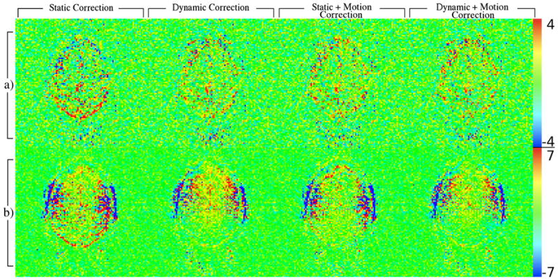
Maps of the regression coefficients for 0.167 Hz sine wave from experiments involving heavy subject breathing at 0.167 Hz (row a) or jaw motion (open/close) at 0.167 Hz (row b) computed after various combinations of field and motion corrections.

Finally, quality of the bulk motion correction parameters calculated by 3dvolreg was evaluated using the root mean square (RMS) error between each volume repetition in the series and the volume used as the base for alignment. A paired t-test of H₀: μ_ERR,stat = μ_ERR,dyn vs. H_a: μ_ERR,stat ≠ μ_ERR,dyn, where μ_ERR,stat and μ_ERR,dyn are the mean RMS error after static and dynamic correction respectively, resulted in p ≪ 0.0001 (t = 6.24) in the heavy breathing experiment and p ≪ 0.0001 (t = 12.73) in the jaw motion experiment. This significantly supports the conclusion that dynamic correction improves subsequent motion correction and, predictably, benefit is increased as the field changes become more spatially inconsistent.

Discussion

The results of our investigations consistently show how temporal changes in the magnetic field can largely confound statistics that rely on models of phase that do not account for these effects. More interestingly, the strikingly positive results of dynamic correction for complex data analysis are demonstrated with a similar consistency, and similar benefits would be expected when using other phase sensitive statistical models (Menon, 2002; Rowe et al., 2007). Additionally, evidence suggests the dynamic correction improves the ability to perform motion correction and can reduce temporal magnitude signal components likely induced by temporal field variations. This is especially true in areas most susceptible to these changes, such as areas of high spatial contrast along the phase encoding direction. However, the data shown reveals little change in the MO activations after performing the correction. When the variation in the magnetic field is relatively constant over space, as often results from breathing, motion correction alone provides comparable results to the dynamic correction in the magnitude signal. However, when the field changes with significant spatial variability, bulk motion correction alone was not able to match the performance of the dynamic field correction. In either case, however, motion correction was improved when applied after the dynamic correction. Also, the indirect effect of bulk motion on phase cannot be removed with bulk motion correction, but the dynamic correction accomplishes this as well.

Better results may be achievable by utilizing more effective correction methods than SPHERE. The inverse approaches (Munger et al., 2000; Liu and Ogawa, 2006) have shown the ability to provide improved intensity correction, especially in the presence of large field gradients. These techniques require field maps estimated in non-warped space, which is not the case for this method, preventing their use. However, investigation into methods of applying these or similar techniques to dynamic field mapping is underway.

This straightforward method requires no additional reference scan, specialized pulse sequences or hardware. In addition, it can be applied to any previously acquired GE-EPI data set where complex data is available. It is, however, only applicable to single shot GE-EPI and can be applied retrospectively. Neglecting computation time, the summation in Eq. (1.2), representing the average phase of all images, could be computed as a running average to enable pseudo-real-time application of the corrections. Possibly the most important potential drawback is the dependence on the temporal invariance in the phase of the radio frequency pulse. However, nearly every multi-shot imaging method relies on this invariance to hold true. However, extreme amounts of movement within the transmit coil can alter its loading and thus the homogeneity of the B₁ field phase. This is unlikely to occur within the range of routine scans (Lamberton et al., 2007), even those requiring small amounts of head movement.

Conclusion

The proposed method for measuring and subsequent correction of MRI time series for effects of temporal dynamics in the main (static) magnetic field has shown impressive ability to restore statistical power to the complex constant phase fMRI activation model. Simulation results also indicate that the dynamic correction results in more robust activation statistics, which more reliably represent the true underlying activation. While it is difficult to directly conclude this from experimental data, there is clear evidence showing reduction in undesired signal components correlating strongly with known temporal magnetic field variations, suggesting this to be the case.

References

- Bandettini PA, Jesmanowicz A, Wong EC, Hyde JS. Processing strategies for time-course data sets in functional MRI of the human brain. Magn Reson Med. 1993;30:161–173. doi: 10.1002/mrm.1910300204. [DOI] [PubMed] [Google Scholar]
- Barry RL, Menon RS. Modeling and suppression of respiration-related physiological noise in echo-planar functional magnetic resonance imaging using global and one-dimensional navigator echo correction. Magn Reson Med. 2005;54:411–8. doi: 10.1002/mrm.20591. [DOI] [PubMed] [Google Scholar]
- Cox RW. AFNI: Software for analysis and visualization of functional magnetic resonance neuroimages. Computers and Biomedical Research. 1996;29:162–173. doi: 10.1006/cbmr.1996.0014. [DOI] [PubMed] [Google Scholar]
- Hu X, Le TH, Parrish T, Erhard P. Retrospective estimation and correction of physiological fluctuation in functional MRI. Magn Reson Med. 1995;34:201–212. doi: 10.1002/mrm.1910340211. [DOI] [PubMed] [Google Scholar]
- Hutton C, Bork A, Josephs O, Deichmann R, Ashburner J, Turner R. Image distortion correction in fMRI: A quantitative evaluation. NeuroImage. 2002;16:217–240. doi: 10.1006/nimg.2001.1054. [DOI] [PubMed] [Google Scholar]
- Jesmanowicz A, Wong EC, Hyde JS. Phase correction of EPI using internal reference lines. Proc. of the 12th Annual Meeting of SMRM; New York. 1993. p. 1239. [Google Scholar]
- Jezzard P, Balaban RS. Correction for geometric distortion in echo planar images from B0 field variations. Magn Reson Med. 1995;34:65–73. doi: 10.1002/mrm.1910340111. [DOI] [PubMed] [Google Scholar]
- Jezzard P, Clare S. Sources of distortion in functional MRI data. Hum Brain Mapp. 1999;8:80–85. doi: 10.1002/(SICI)1097-0193(1999)8:2/3<80::AID-HBM2>3.0.CO;2-C. [DOI] [PMC free article] [PubMed] [Google Scholar]
- Kadah YM, Hu X. Simulated phase evolution rewinding (SPHERE): a technique for reducing B0 inhomogeneity effects in MR images. Magn Reson Med. 1997;38:615–627. doi: 10.1002/mrm.1910380416. [DOI] [PubMed] [Google Scholar]
- Kannengiesser SA, Wang Y, Haacke EM. Geometric distortion correction in gradient-echo imaging by use of dynamic time warping. Magn Reson Med. 1999;42:585–590. doi: 10.1002/(sici)1522-2594(199909)42:3<585::aid-mrm22>3.0.co;2-a. [DOI] [PubMed] [Google Scholar]
- Lamberton F, Delcroix N, Grenier D, Mazoyer B, Joliot M. A new EPI-based dynamic field mapping method: application to retrospective geometrical distortion corrections. J Magn Reson Imaging. 2007;26:747–755. doi: 10.1002/jmri.21039. [DOI] [PubMed] [Google Scholar]
- Lin LI. A concordance correlation coefficient to evaluate reproducibility. Biometrics. 1989;45:255–268. [PubMed] [Google Scholar]
- Liu G, Ogawa S. EPI image reconstruction with correction of distortion and signal losses. J Magn Reson Imaging. 2006;24:683–689. doi: 10.1002/jmri.20672. [DOI] [PubMed] [Google Scholar]
- Logan BR, Rowe DB. An evaluation of thresholding techniques in fMRI analysis. NeuroImage. 2004;22:95–108. doi: 10.1016/j.neuroimage.2003.12.047. [DOI] [PubMed] [Google Scholar]
- Menon RS. Postacquisition suppression of large-vessel BOLD signals in high-resolution fMRI. Magn Reson Med. 2002;47:1–9. doi: 10.1002/mrm.10041. [DOI] [PubMed] [Google Scholar]
- Munger P, Crelier GR, Peters TM, Pike GB. An inverse problem approach to the correction of distortion in EPI images. IEEE Trans Med Imaging. 2000;19:681–689. doi: 10.1109/42.875186. [DOI] [PubMed] [Google Scholar]
- Nencka AS, Rowe DB. Reducing the unwanted draining vein BOLD contribution in fMRI with statistical post-processing methods. NeuroImage. 2007;37:177–188. doi: 10.1016/j.neuroimage.2007.03.075. [DOI] [PubMed] [Google Scholar]
- Ogawa S, Lee TM, Kay AR, Tank DW. Brain magnetic resonance imaging with contrast dependent on blood oxygenation. Proc Natl Acad Sci USA. 1990;87:9868–9872. doi: 10.1073/pnas.87.24.9868. [DOI] [PMC free article] [PubMed] [Google Scholar]
- Reber PJ, Wong EC, Buxton RB, Frank LR. Correction of off resonance-related distortion in echo-planar imaging using EPI-based field maps. Magn Reson Med. 1998;39:328–330. doi: 10.1002/mrm.1910390223. [DOI] [PubMed] [Google Scholar]
- Robson MD, Gore JC, Constable RT. Measurement of the point spread function in MRI using constant time imaging. Magn Reson Med. 1997;38:733–740. doi: 10.1002/mrm.1910380509. [DOI] [PubMed] [Google Scholar]
- Roopchansingh V, Cox RW, Jesmanowicz A, Ward BD, Hyde JS. Single-shot magnetic field mapping embedded in echo-planar time-course imaging. Magn Reson Med. 2003;50:839–843. doi: 10.1002/mrm.10587. [DOI] [PubMed] [Google Scholar]
- Rowe DB. Modeling both the magnitude and phase of complex-valued fMRI data. NeuroImage. 2005;(25):1310–1324. doi: 10.1016/j.neuroimage.2005.01.034. [DOI] [PubMed] [Google Scholar]
- Rowe DB, Logan BR. A complex way to compute fMRI activation. NeuroImage. 2004;23:1078–1092. doi: 10.1016/j.neuroimage.2004.06.042. [DOI] [PubMed] [Google Scholar]
- Rowe DB, Logan BR. Complex fMRI analysis with unrestricted phase is equivalent to a magnitude-only model. NeuroImage. 2005;24:603–606. doi: 10.1016/j.neuroimage.2004.09.038. [DOI] [PubMed] [Google Scholar]
- Rowe DB, Meller CP, Hoffmann RG. Characterizing phase-only fMRI data with an angular regression model. J Neurosci Methods. 2007;161:331–341. doi: 10.1016/j.jneumeth.2006.10.024. [DOI] [PMC free article] [PubMed] [Google Scholar]
- Van de Moortele PF, Pfeuffer J, Glover GH, Ugurbil K, Hu X. Respiration-induced B0 fluctuations and their spatial distribution in the human brain at 7 Tesla. Magn Reson Med. 2002;47:888–895. doi: 10.1002/mrm.10145. [DOI] [PubMed] [Google Scholar]
- Van Gelderen P, de Zwart JA, Starewicz P, Hinks RS, Duyn JH. Real-time shimming to compensate for respiration-induced B0 fluctuations. Magn Reson Med. 2007;57:362–368. doi: 10.1002/mrm.21136. [DOI] [PubMed] [Google Scholar]
- Zeng H, Gatenby JC, Zhao Y, Gore JC. New approach for correcting distortions in echo planar imaging. Magn Reson Med. 2004;52:1373–1378. doi: 10.1002/mrm.20297. [DOI] [PubMed] [Google Scholar]