Model‐based clustering of meta‐analytic functional imaging data

Abstract

We present a method for the analysis of meta‐analytic functional imaging data. It is based on Activation Likelihood Estimation (ALE) and subsequent model‐based clustering using Gaussian mixture models, expectation‐maximization (EM) for model fitting, and the Bayesian Information Criterion (BIC) for model selection. Our method facilitates the clustering of activation maxima from previously performed imaging experiments in a hierarchical fashion. Regions with a high concentration of activation coordinates are first identified using ALE. Activation coordinates within these regions are then subjected to model‐based clustering for a more detailed cluster analysis. We demonstrate the usefulness of the method in a meta‐analysis of 26 fMRI studies investigating the well‐known Stroop paradigm. Hum Brain Mapp, 2008. © 2007 Wiley‐Liss, Inc.

INTRODUCTION

Functional neuroimaging has become a powerful tool in cognitive neuroscience, which enables us to investigate the relationship between particular cortical activations and cognitive tasks performed by a test subject or patient. However, the rapidly growing number of imaging studies still provides a quite variable picture, in particular of higher‐order brain functioning. Considerable variation can be observed in the results of imaging experiments addressing even closely related experimental paradigms. The analysis of the consistency and convergence of results across experiments is therefore a crucial prerequisite for correct generalizations about human brain functions. This calls for analysis techniques on a meta‐level, i.e. methods that facilitate the post‐hoc combination of results from independently performed imaging studies. Moreover, functional neuroimaging is currently advancing from the simple detection and localization of cortical activation to the investigation of complex cognitive processes and associated functional relationships between cortical areas. Such research questions can no longer be addressed by the isolated analysis of single experiments alone, but necessitate the consolidation of results across different cognitive tasks and experimental paradigms. This again makes meta‐analyses an increasingly important part in the evaluation of functional imaging results. Several methodological approaches to the automated meta‐analysis of functional imaging data have recently been proposed, for example, by Turkeltaub et al. (2002); Chein et al. (2002); Nielsen and Hansen (2004); Nielsen (2005); Neumann et al. (2005); Lancaster et al. (2005) and Laird et al. (2005a).

In coordinate‐based meta‐analyses activation coordinates reported from independently performed imaging experiments are analyzed in search of functional cortical areas that are relevant for the investigated cognitive function. In this article we propose to apply a combination of Activation Likelihood Estimation (ALE) and model‐based clustering to this problem. The former is a form of kernel density estimation, which was recently adapted for the automated meta‐analysis of functional imaging data (Chein et al., 2002; Turkeltaub et al., 2002). The latter provides a general framework for finding groups in data by formulating the clustering problem in terms of the estimation of parameters in a finite mixture of probability distributions (Everitt et al., 2001; Fraley and Raftery, 2002). In the context of functional imaging, mixture modeling has been used previously for the detection of brain activation in single‐subject functional Magnetic Resonance Imaging (fMRI) data. For example, Everitt and Bullmore (1999) modeled a test statistic estimated at each voxel as mixture of central and non‐central χ ² distributions. This approach was extended by Hartvig and Jensen (2000) to account for the spatial coherency of activated regions. Penny and Friston (2003) used mixtures of General Linear Models in a spatio‐temporal analysis in order to find clusters of voxels showing task‐related activity.

The combination of model‐based clustering and ALE presented in this article should be viewed as an extension rather than a replacement of ALE, which is currently the state‐of‐the‐art approach to the meta‐analysis of functional imaging data. ALE is based on representing activation maxima from individual experiments by three‐dimensional Gaussian probability distributions from which activation likelihood estimates for all voxels can be inferred. These estimates are then compared to a null‐distribution derived from permutations of randomly placed activation maxima. Successful application of ALE has been demonstrated by Chein et al. (2002); Turkeltaub et al. (2002); Wager et al. (2004), and by several authors contributing to Fox et al. (2005). However, one drawback of the method in its current form is its strong dependency on the standard deviation of the Gaussian. Choosing the standard deviation too small results in many small activation foci which cover only a small part of the original input data and do not carry significantly more information than provided by the individual activation maxima alone. In contrast, using a large standard deviation results in activation foci, which represent more of the original activation maxima. However, as will be seen in our experimental data, the size of such foci can by far exceed the extent of corresponding activations typically found in single fMRI studies. Such ALE foci might thus comprise more than one functional unit. This can be observed, in particular, in studies with a very inhomogeneous distribution of activation coordinates. In this case a certain adaptiveness of the method or a hierarchical approach would be desirable.

We propose to alleviate this problem by first applying ALE to the original data and then subjecting activation maxima lying within the resulting activation foci to further clustering. Using a large standard deviation of the Gaussian in the first step yields a new set of activation maxima from which coordinates with no other activation maxima in their vicinity are removed. The subsequent model‐based clustering then explores the statistical distribution of the remaining coordinates.

Model‐based clustering assumes that the observed data are generated by a finite mixture of underlying probability distributions. Each probability distribution corresponds to a cluster. Our particular implementation closely follows the general model‐based clustering approach proposed by Fraley and Raftery (2002). This approach considers mixtures of multivariate Gaussians. Maximum likelihood estimation of the mixture models is performed via the expectation‐maximization (EM) algorithm (Hartley, 1958; Dempster et al., 1977), which determines the parameters of the mixture components as well as the posterior probability for a data point to belong to a specific component or cluster. Since a suitable initialization is critical in the successful application of EM, hierarchical agglomerative clustering is performed as an initializing step.

Varying the parameterization of the covariance matrix of a Gaussian mixture provides a set of models with different geometric characteristics, reaching from spherical components of equal shape and volume to ellipsoidal components with variable shape, volume, and orientation (Banfield and Raftery, 1993). We use a set of 10 different parameterizations. The best parameterization of the model and the optimal number of clusters are determined using the Bayesian Information Criterion (BIC) (Schwarz, 1978).

In the following, we provide the methodological background of ALE, Gaussian mixture models, and BIC for model selection. We then present experimental data showing the application of the method in a meta‐analysis of 26 fMRI experiments investigating the well‐known Stroop paradigm.

METHODS

ALE

ALE, concurrently but independently developed by Turkeltaub et al. (2002) and Chein et al. (2002), was among the first methods aimed at modeling cortical areas of activation from meta‐analytic imaging data. It was recently extended by Laird et al. (2005a) to account for multiple comparisons and to enable statistical comparisons between two or more meta‐analyses. Moreover, it has been used in combination with replicator dynamics for the analysis of functional networks in meta‐analytic functional imaging data (Neumann et al., 2005). For the presented meta‐analysis, ALE was implemented as part of the software package LIPSIA (Lohmann et al., 2001).

In ALE, activation maxima are modeled by three‐dimensional Gaussian probability distributions centered at their Talairach coordinates. Specifically, the probability that a given activation maximum lies within a particular voxel is

(1)

where σ is the standard deviation of the distribution and d is the Euclidean distance of the voxel to the activation maximum. For each voxel, the union of these probabilities calculated for all activation maxima yields the ALE. In regions with a relatively high density of reported activation maxima, voxels will be assigned a high ALE in contrast to regions where few and widely spaced activation maxima have been reported.

From the resulting ALE maps, one can infer whether activation maxima reported from different experiments are likely to represent the same functional activation. A non‐parametric permutation test is utilized to test against the null‐hypothesis that the activation maxima are spread uniformly throughout the brain. Given some desired level of significance α, ALE maps are thresholded at the 100(1−α)th percentile of the null‐distribution. Topologically connected voxels with significant ALE values are then considered activated functional regions.

The extent and separability of the resulting regions critically depends on the choice of σ in Eq. (1). As observed, for example, by Derrfuss et al. (2005), decreasing σ leads to smaller regions of significant voxels and to an increase in the number of discrete above threshold regions which, however, represent only few of the original activation maxima. Increasing σ has the opposite effect with larger regions representing more of the original data. Most commonly σ is chosen to correspond to the size of spatial filters typically applied to fMRI data. In previously published ALE analyses (see Fox et al. (2005) for some examples) we found σ to vary between 9.4 and 10 mm FWHM, in rare cases 15 mm were used. In the vast majority of analyses, the standard deviation of the Gaussian was set to 10 mm FWHM. As we view ALE as a pre‐processing step to model‐based clustering, the activation likelihood should not be estimated too conservatively. Therefore, we use a relatively large standard deviation of σ = 5 mm, corresponding to 11.8 mm FWHM.

Model‐Based Clustering

ALE leads to a reduced list of activation maxima containing only those maxima which have one or more other maxima in their vicinity. These coordinates are then subjected to clustering based on a finite mixture of probability distributions. Here, we will closely follow the procedure suggested by Fraley and Raftery (1998, 2002), who propose a group of Gaussian mixture models, maximum likelihood estimation via EM, hierarchical agglomeration as initial clustering, and model and parameter selection via BIC. In the following, the individual parts of the clustering procedure are described in detail. These parts were implemented for our application using the software package MCLUST (Fraley and Raftery, 1999, 2003).

Gaussian Mixture Models

For n independent multivariate observations x = (x ₁, …, x_n), the likelihood of a mixture model with M components or clusters can be written as

(2)

where f _k is the density of the cluster k with parameter vector θ _k, and p = (p ₁,…,p _M) is the vector of mixing proportions with p _k ≥ 0 and ∑_k p _k = 1. Since any distribution can be effectively approximated by a mixture of Gaussians (Silverman, 1985; Scott, 1992), the probability density function is most commonly represented by

(3)

for d‐dimensional data with mean μ _k and covariance matrix Σ_k. Geometrical features of the components can be varied by parameterization of the covariance matrices Σ_k. Banfield and Raftery (1993) suggest various parameterizations through the eigenvalue decomposition

(4)

D _k is the matrix of eigenvectors, A _k is a diagonal matrix with elements that are proportional to the eigenvalues of Σ_k such that |A _k| = 1, and λ _k is a scalar. Treating D _k, λ _k, and A _k as independent parameters and keeping them either constant or variable across clusters varies the shape, volume, and orientation of the components. In the simplest case Σ_k = λI, all clusters are spherical and of equal size. The least constraint case given in Eq. (4) accounts for ellipsoidal clusters of variable shape, volume, and orientation. All parameterizations available in MCLUST and applied to our experimental data are presented in Table I. The first two models have spherical, all other models have ellipsoidal components, whereby components in models with diagonal covariance matrices (c–f) are oriented along the coordinate axes. Models with identical matrix A for all components have equally shaped components, whereas models with identical λ for all components have components of the same volume.

Table I.

Parameterization of the covariance matrices

Parameterization	Components
	Shape	Volume	Orientation
a) Σk = λI	Equal	Equal	—
b) Σk = λ k I	Equal	Variable	—
c) Σk = λA	Equal	Equal	Along the coordinate axes
d) Σk = λ k A	Equal	Variable	Along the coordinate axes
e) Σk = λkA k	Variable	Equal	Along the coordinate axes
f) Σk = λ k A k	Variable	Variable	Along the coordinate axes
g) Σk = λDAD T	Equal	Equal	Equal
h) Σk = λD k AD k T	Equal	Equal	Variable
i) Σk = λ k D k AD k T	Equal	Variable	Variable
k) Σk = λ k D k A k D k T	Variable	Variable	Variable

The table shows the different parameterizations applied in model‐based clustering. It can be seen that A _k accounts for the shape of a component, λ _k for its volume, and D _k for its orientation. Table adapted from Table I in Fraley and Raftery (1999).

Maximum Likelihood Estimation

Maximum likelihood estimation of a Gaussian mixture model as defined in Eqs. (2) and (3) can be performed via the widely used EM algorithm, which provides a general approach to parameter estimation in incomplete data problems (Dempster et al., 1977; Hartley, 1958; Neal and Hinton, 1998). In general, given a likelihood function L(θ|y) = Π f (y _i|θ), for parameters θ and data y = (y ₁, …, y _n), we wish to find such that

In the presence of some hidden data z such that y = (x,z) with x observed and z unobserved, we can equivalently maximize the so‐called complete‐data log likelihood and find such that

Starting from an initial guess, the EM algorithm proceeds by alternately estimating the unobservable data z and the unknown parameters θ. Specifically, in the E‐step, the algorithm calculates the expected value of the complete‐data log likelihood with respect to z given x and the current estimate of θ. In the M‐step, this expected value is maximized in terms of θ, keeping z fixed as computed in the previous E‐step.

In our application, the complete data y = (y ₁, …, y _n), consists of y _i = (x _i,z _i) where each x _i is a three‐dimensional vector containing coordinates of activation maxima in Talairach space and z _i = (z _i1,…,z _iM) is the unknown membership of x _i in one of the M clusters, i.e.

With the density of observation x _i given z _i written as Π_k f _k(x _i|μ _k,Σ_k)^zik, the complete‐data log likelihood in our problem can be formulated as

(5)

assuming that each z _i is independently and identically distributed according to a multinomial distribution of one draw from M categories with probabilities p ₁, …, p _M (Fraley and Raftery, 1998).

Maximum likelihood estimation is performed by alternating between the calculation of z _ik given x _i, μ _k, and Σ_k (E‐step) and maximizing Eq. (5) with respect to μ _k, Σ_k, and p _k with z _ik fixed (M‐step). Mathematical details of the algorithm are given in Appendix A. The EM algorithm terminates after the difference between successive values of ℓ falls below some threshold ϵ, which in our application was set to ϵ = 0.00001. The value of z _ik at the maximum of Eq. (5) is the estimated probability that x _i belongs to cluster k, and the maximum likelihood classification of x _i is the cluster k, with

Initialization by Hierarchical Agglomeration

Following the suggestion by Fraley and Raftery (1998), we employ model‐based hierarchical agglomeration provided in MCLUST as initializing partitioning method. This method tends to yield reasonable clusterings in the absence of any information about a possible clustering inherent in the data (Fraley and Raftery, 2002).

Hierarchical agglomeration techniques typically start with a pre‐defined number of clusters and in each step merge the two closest clusters into a new cluster, thereby reducing the number of clusters by one. The implementation used here starts with n clusters, each containing a single observation x _i. Then, two clusters are chosen such that merging them increases the so‐called classification likelihood, given as

(6)

with f _k(x _i) given in Eq. (3). The vector c = (c ₁, …, c _n) encodes the classification of the data, i.e. c _i = k, if x _i is classified as member of cluster k. For an unrestricted covariance matrix as defined in Eq. (4), approximately maximizing the classification likelihood (6) amounts to minimizing

where n _k is the number of elements in cluster k and W _k is the within‐cluster scattering matrix of cluster k as defined in Eq. (8) in Appendix A (Banfield and Raftery, 1993). Computational issues on this clustering procedure are discussed in detail by Banfield and Raftery (1993) and Fraley (1998), in particular regarding the initial stages with a single data point in each cluster, which leads to |W| = 0.

From the values of c at the maximum of C, initializations for the unknown membership values z _ik are derived, and first estimates for the parameters of the Gaussian components can be obtained from an M‐step of the EM algorithm as described in Appendix A.

Model Selection via BIC

A problem of most clustering techniques is to determine the number of clusters inherent in the data. One common technique in model‐based clustering is to apply several models with different pre‐defined numbers of components and subsequently choose the best model according to some model selection criterion. For models with equal number of parameters, the simplest approach is to compare estimated residual variances. This is not applicable, however, when models with varying number of parameters are considered.

An advantage of using mixture models for clustering is that approximate Bayes factors can be used for model selection. Bayes factors were developed originally as a Bayesian approach to hypothesis testing by Jeffreys (1935, 1961). In the context of model comparison, a Bayes factor describes the posterior odds for one model against another given equal prior probabilities. It is determined from the ratio of the integrated likelihoods of the models. In conjunction with EM for maximum likelihood estimation, the integrated likelihood of a model can be approximated under certain regularity conditions by the BIC (Schwarz, 1978), which is defined as

(7)

where is the maximized mixture log likelihood of the model, m is the number of independent parameters of the model, and n the number of data points. With this definition, a large BIC value provides strong evidence for a model and the associated number of clusters.

The relationship between Bayes factors and BIC, the regularity conditions, and the use of Bayes factors for model comparison are discussed in more detail, e.g., by Kass and Raftery (1995). They also provide guidelines for the strength of evidence for or against some model: A difference of less than 2 between the BIC of two models corresponds to weak, a difference between 2 and 6 to positive, between 6 and 10 to strong, and a difference greater than 10 to very strong evidence for the model with the higher BIC value.

Putting Things Together

Taking together the individual parts described above, our algorithm for deriving activated functional regions from meta‐analytic imaging data can be summarized as follows:

• 1Given a list of coordinates encoding activation maxima in Talairach space from a number of individual studies, calculate ALEs for all voxels using a large standard deviation of the Gaussian. Determine those coordinates that fall within the regions above the ALE threshold.
• 2Determine a maximum number of clusters M. Perform hierarchical agglomeration for up to M clusters using the reduced coordinate list obtained in Step 1 as input, thereby approximately maximizing the classification likelihood as defined in Eq. (6).
• 3For each parameterization and number of clusters of the model as defined in Eq. (5) perform EM, using the classification obtained in Step 2 as initialization.
• 4Calculate the BIC for each parameterization and number of clusters in the model according to Eq. (7)
• 5Choose the parameterization and number of clusters with a decisive maximum BIC value as solution according to the guidelines above.

Experimental Data

Our method was applied in a meta‐analysis of 26 fMRI experiments employing the well‐known Stroop paradigm (Stroop, 1935). A list of included studies is given in Appendix B. The Stroop paradigm is designed to investigate interference effects in the processing of a stimulus while a competing stimulus has to be suppressed. For example, subjects are asked to name a color word, say “red,” which is presented on a screen in the color it stands for (congruent condition) or in a different color (incongruent condition). Other variants of the Stroop paradigm include the spatial word Stroop task (the word “above” is written below a horizontal line), the counting Stroop task (the word “two” appears three times on the screen) and the object‐color Stroop task (an object is presented in an atypical color, e.g. a blue lemon).

This particular paradigm was chosen as a test case for our method, because the interference effect and the associated cortical activations are known to be produced very reliably. Activations are most commonly reported in the left inferior frontal region, the left inferior parietal region, and the left and right anterior cingulate (Banich et al., 2000; Liu et al., 2004; McKeown et al., 1998). Our own previous meta‐analysis based on ALE and subsequent application of replicator dynamics (Neumann et al., 2005) revealed a frontal network including the presupplementory motor area (preSMA), the inferior frontal sulcus (IFS) extending onto the middle frontal gyrus, the anterior cingulate cortex (ACC) of both hemispheres, and the inferior frontal junction area (IFJ). Other frequently reported areas include frontopolar cortex, occipital cortex, fusiform gyrus, and insula (Laird et al., 2005b; Zysset et al., 2001).

Despite the high agreement in the reported activated areas, the actual location of associated coordinates in Talairach space differs widely between studies. For example, the left IFJ was localized in previous studies at Talairach coordinates x between −47 and −35, y between −4 and 10, and z between 27 and 40 (Brass et al., 2005; Derrfuss et al., 2004, 2005; Neumann et al., 2005). Such high variability makes the classification of the data into distinct functional units difficult.

We applied our analysis to data extracted from the BrainMap database (Fox and Lancaster, 2002). This database provides Talairach coordinates of activation maxima from functional neuroimaging experiments covering a variety of experimental paradigms and imaging modalities. At the time of writing the database contained over 27,500 activation coordinates reported in 790 papers.

Searching the database for fMRI experiments investigating the Stroop interference task resulted in 26 peer‐reviewed journal publications. Within these studies, 728 Talairach coordinates for activation maxima were found. The majority of these coordinates (550 out of 728) represented the Stroop interference effect, i.e. significant activation found for the contrasts incongruent ≥ congruent, incongruent ≥ control, or incongruent + congruent ≥ control. As control condition, either the presentation of a neutral object (e.g. “XXXX” instead of a color word) or a simple visual fixation were used. Fifty‐five coordinates were marked as deactivation in the database, i.e. they represent the contrast congruent ≥ incongruent. The remaining coordinates were reported to represent other contrasts such as the contrast between different Stroop modalities or a conjunction of Stroop interference, spatial interference, and the Flanker task. Note that 26 coordinates came from a meta‐analysis on Stroop interference, nine coordinates represented the interference effect in pathological gamblers, and all remaining coordinates were taken from group studies with healthy subjects.

As the focus of our work is on the development of meta‐analysis tools rather than the investigation of the Stroop paradigm, all 728 coordinates were subjected to the subsequent analysis without any further selection. This not only enabled us to test our method on a reasonably large data set, it also introduced some “realistic” noise into our data.

Plots of all coordinates projected onto a single axial, sagittal, and coronal slice are shown in the top row of Figure 1. Coordinates reported from different studies are represented by different colors. As can be seen, activation maxima are distributed over large parts of the cortex, although some areas with a higher density of activation coordinates are already apparent, in particular in the left lateral prefrontal cortex and the medial frontal cortex. These can be seen more clearly in the example slices in the bottom row of Figure 1.

Figure 1.

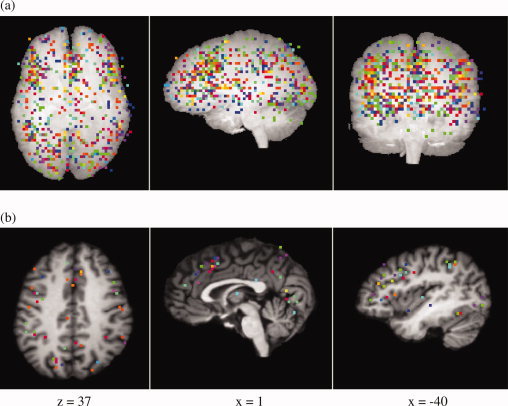
(a) 728 activation coordinates which were included in the analysis, projected onto three orthogonal single coronal, sagittal, and axial slices. (b) Three example slices showing activation coordinates projected onto an individual brain. Slices were chosen to show cortical areas which are frequently reported as significantly activated in the Stroop task (ACC, IFJ, preSMA). Activation coordinates from the same study are plotted in the same color. [Color figure can be viewed in the online issue, which is available at www.interscience.wiley.com.]

Experimental Results

Activation coordinates were first subjected to an ALE analysis with standard deviations of σ = 5 mm, corresponding to 11.8 mm FWHM. The null distribution was derived from 1,000 iterations of randomly placing 728 activation coordinates over a mask brain volume defined by the minimum and maximum Talairach coordinates in the original data set. The brain mask spanned a volume of 61,408 voxels, each 3 × 3 × 3 mm³ in size. As suggested by Turkeltaub et al. (2002), the resulting ALE map was thresholded at an α‐level of α = 0.01%. This corresponded to an ALE threshold of 0.0156. Figure 2 shows sagittal and axial example slices of the ALE map containing only voxels above threshold.

Figure 2.

ALE maps derived from 728 activation coordinates reported for the Stroop paradigm. The ALE map was thresholded at α = 0.01% yielding a maximum ALE value of ALEmax = 0.049. Axial and sagittal slices correspond to the example slices shown in Figure 1b. [Color figure can be viewed in the online issue, which is available at www.interscience.wiley.com.]

The ALE analysis yielded 13 regions of topologically connected voxels above threshold, which covered a total volume of 54,810 mm³ and contained 210 of the original activation maxima. Table II shows size, maximum ALE value, location of the center in Talairach space, and the number of original activation coordinates covered by the detected ALE regions.

Table II.

ALE regions obtained for 728 activation maxima

Volume	Max ALE	Location	Number of coordinates
19,494	0.05	L(−44 6 33)	66
13,716	0.05	R(1 18 39)	49
9,882	0.04	R(43 9 30)	36
6,048	0.03	L(−41 −51 45)	25
3,105	0.03	L(−38 −72 3)	16
1,134	0.02	L(−47 −54 −3)	7
297	0.02	R(49 −45 30)	3
324	0.02	L(−5 36 −3)	2
297	0.02	R(46 −51 −6)	1
189	0.02	R(10 −60 15)	2
162	0.02	R(7 −75 −9)	1
81	0.02	R(19 48 21)	1
81	0.02	R(37 −72 −3)	1

The table shows ALE regions and the number of activation coordinates falling within these regions as result of the ALE analysis of 728 activation maxima representing 26 Stroop studies. Regions are ordered by size.

Note that the four largest regions cover 89.65% (49,140 mm³) of the total ALE regions' volume. They contain 83.8% of all above‐threshold coordinates. This can be explained by the very inhomogeneous distribution of the original input coordinates: More than 40% of the original activation maxima fell within regions spanned by the minimum and maximum Talairach coordinates of the four largest ALE regions. The remaining coordinates were distributed more evenly over other parts of the cortex.

Note further that some smaller regions surviving the ALE threshold contain only single activation maxima. This seems counterintuitive at first, as a single coordinate should not result in a relatively high ALE value. However, imagine, for example, a situation where three coordinates are arranged in a “row,” i.e. at three voxels in the same row of a slice with one voxel between them. The voxel in the middle will get a higher empirical ALE value than the ones at both ends, as it has two other coordinates in close distance (only two voxels away) whereas the other two voxels have one coordinate in close distance and another one four voxels further away. Depending on the distribution of other coordinates, thresholding the ALE values could now shape the surviving ALE region such that only the coordinate in the middle will be inside the region, whereas the value at the other two voxels might just be too small to survive the thresholding. Thus, ALE regions containing only a single coordinate are caused by very small groups of activation maxima that are quite isolated from the remaining ones. The fact that some of our ALE regions contain only a single coordinate indicates that all remaining activation coordinates, not surviving the thresholding, are very isolated from each other. They can therefore be regarded as noise.

Despite the use of a very small α‐level in ALE thresholding, some of the determined ALE foci clearly exceed the size of cortical activations typically found in these regions for the Stroop paradigm (see, e.g. Zysset et al. (2001) for a comparison). Moreover, as seen in Figure 2, within such foci, in particular in the left prefrontal cortex, sub‐maxima of ALE values are visible, indicating a possible sub‐clustering of the represented activation coordinates. All above‐threshold activation coordinates were therefore subjected to model‐based clustering as the second part of our method.

Hierarchical agglomeration of the above‐threshold coordinates was first performed for up to 30 clusters. Using the results as initialization for the EM algorithm, models as defined in Eq. (5) with the parameterizations introduced in Section Model‐Based Clustering with up to 30 clusters were then applied to the data set, and BIC values were calculated for each number of clusters and parameterization.

The three models with λ _k = λ, i.e. models with components of equal volume, outperformed the remaining models, which all allowed for components of variable volume. This seems counterintuitive at first, as a more variable model would be expected to fit the data better than a more restricted one. However, as described above, the BIC value penalizes model complexity, which is larger for models with variable components than for models with equal components. Thus, for our data, allowing the components' volume to vary did not increase the log likelihood of the models sufficiently in order to justify the increased number of model parameters. Note also that for very large cluster numbers, some more variable models failed to provide a clustering due to the singularity of the associated covariance matrices. This was not the case for models with fewer free parameters, however.

Figure 3 shows plots of the BIC values of the best three models for up to 30 clusters. BIC values of these models are very similar, in particular for models with more than 20 clusters. The right side shows an enlarged plot of the BIC values for models with 20 up to 25 clusters. All three models yielded the highest BIC value when applied with 24 clusters. The more complex models with ellipsoidal components slightly outperformed the spherical one, whereby the difference between a variable and a fixed orientation of the components was negligible.

Figure 3.

Plot of the BIC values of the best three models for up to 30 clusters (left) and enlarged plot of the BIC values for the best three models with cluster numbers between 20 and 25 (right). [Color figure can be viewed in the online issue, which is available at www.interscience.wiley.com.]

Figure 4 shows the results of the model‐based clustering exemplified for the two largest ALE regions, which were situated in the left lateral prefrontal cortex (left LPFC) and the medial frontal cortex (MFC), respectively (cf. Table II). The categorization of activation coordinates within the left LPFC is shown in five consecutive sagittal functional slices at Talairach coordinates between x = −34 and x = −46. The coordinates in this ALE region were subdivided into five groups in anterior‐posterior and superior‐inferior direction. In the most posterior and superior part of the region a further division in lateral‐medial direction can be observed (shown in green and blue). Interestingly, cluster centers of the more anterior and inferior clusters corresponded closely to the sub‐maxima in the ALE focus visible in Figure 2. However, the division of posterior and superior parts of the region into two clusters could not have been predicted from the ALE sub‐maxima. The same holds for the clustering of coordinates in the MFC, where no sub‐maxima could be observed in the ALE map. The categorizations of coordinates in the MFC is shown in the right panel of Figure 4 in four consecutive sagittal slices. The best model provided four clusters, again dividing the region in anterior‐posterior and superior‐inferior direction. Thus, model‐based clustering revealed some additional structure in the data that would have remained undetected when using ALE alone. To get some feeling for the actual shape of the clusters and their relative location, the extracted clusters are presented again in views from different angles in Figure 5.

Figure 4.

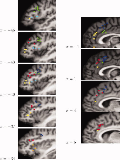
Left: Clustering results for the largest ALE region (left LPFC), shown in five consecutive sagittal slices. The clustering yielded five clusters (shown in green, light blue, yellow, red, and blue), dividing the region primarily in anterior‐posterior and superior‐inferior direction. The most posterior and superior part of the region was further divided in lateral‐medial direction. An additional cluster centered around the left insula can be seen in orange at x= −34. These coordinates were not part of the largest ALE region. Right: Results for the second largest ALE region (MFC) shown in four consecutive sagittal slices. Clustering yielded four clusters (blue, green, yellow, red), again dividing the region in anterior‐posterior and superior‐inferior direction. Note that the single coordinate shown in orange at x = −1 was not part of the second largest ALE region. [Color figure can be viewed in the online issue, which is available at www.interscience.wiley.com.]

Figure 5.

Clustering results, on the left for the largest ALE region (left LPFC) and on the right for the second largest ALE region (MFC). Clusters are shown in a sagittal view (top) corresponding to the view in Figure 4 and twice turned around the y axis by a few degrees in order to visualize the shape and separation of the clusters. Colors correspond to the colors in Figure 4. [Color figure can be viewed in the online issue, which is available at www.interscience.wiley.com.]

The robustness of our method against noisy input data was tested in a post‐hoc analysis including only the 550 activation coordinates that truly represented the Stroop interference effect. The results did not significantly differ from the results of the original analysis. The noise in the original input data thus did not have a noteworthy impact on the results of the model‐based clustering.

DISCUSSION

ALE facilitates the detection of cortical activation from activation maxima reported in independently performed functional imaging studies. The resulting areas reflect the distribution of activation maxima over the cortex. In particular, clusters of activation maxima in a region reflect the likely involvement of this region in processing a cognitive task, whereas isolated activation maxima are regarded as noise.

Our analysis shows that the extent of ALE regions can vary considerably due to the heterogeneous distribution of the input data across different parts of the cortex. As seen in Table II and Figure 2, the size of some ALE foci obtained in the first step of our analysis by far exceeded the extent of comparable activations reported in single fMRI experiments. For example, activation maxima reported by Zysset et al. (2001) for two separated activations in the posterior (Tal: −38, 5, 30) and the anterior (Tal: −38, 35, 5) inferior frontal sulcus are both located within the same ALE region in our analysis. This is caused by the high number of activation coordinates within this region together with their high spatial variability. Moreover, within the largest ALE focus located in the left LPFC, sub‐maxima could be observed, indicating a possible sub‐clustering of the region.

One simple way to separate several areas within such a large ALE region would be the choice of a higher ALE threshold. However, this is problematic if a whole brain analysis is performed, since ALE values in other regions might be significantly lower despite a high concentration of activation coordinates. For example, in Figure 2b a cluster of activation coordinates can clearly be seen in the anterior part of the left intraparietal sulcus. However, the resulting ALE focus representing no less than 25 activation coordinates has a maximum ALE value of only 0.027 in comparison to 0.05 in the left LPFC. Thus, by simply choosing a higher ALE threshold, some clusters of activation coordinates might remain undetected.

We tried to alleviate this problem by following a hierarchical approach. In a first step, ALE is used to identify regions with high concentration of activation coordinates. In a second step, large ALE regions are further investigated in search for a possible sub‐division.

Applying this two‐step procedure to activation maxima from 26 Stroop experiments first resulted in relatively large ALE regions, in particular in the frontal lobe (cf. Fig. 2). This is in line with earlier findings on frontal lobe activity, in particular in a meta‐analysis by Duncan and Owen (2000) who reported cortical regions of large extent to be recruited by a variety of cognitive tasks. However, in contrast to this study, our analysis pointed to a possible further sub‐clustering of these areas. The two largest ALE regions found in the left lateral prefrontal cortex and the medial frontal wall were partitioned into five and four clusters, respectively. While our exploratory analysis technique does not have the power to associate specific cognitive functions to these clusters, this finding could serve as a hypothesis for a further functional specialization of these regions.

The main directions of the clustering were in parallel to the coordinate axes, primarily in anterior‐posterior and superior‐inferior direction. This corresponds well with recent results from single‐subject and group analyses obtained from a variety of analysis techniques as well as from other meta‐analyses, see e.g. Neumann et al. (2006); Forstmann et al. (2005); Koechlin et al. (2003); Müller et al. (2003) for LPFC, and Forstmann et al. (2005) and Amodio and Frith (2006) for MFC clustering.

It is important to be clear about the implicit assumptions made in the application of our analysis technique. Meta‐analyses are aimed at consolidating results from several studies in order to find general mechanisms related to a particular task, class of paradigms, etc. Thus, if we want to generalize the findings of any meta‐analysis, we must assume that the data extracted from the included studies are a representative sample of all the data collected for the investigated phenomenon. Note, however, that this must be assumed in any empirical analysis relying on sampled data. A second, closely related, assumption specific to clustering activation coordinates is that the inherent distribution of activation for the investigated phenomenon is completely represented by the investigated data.

In a meta‐analysis, these assumptions are sometimes hard to meet because of the selective publication of activation coordinates from particular cortical regions, a problem often referred to as “publication or literature bias.” In the majority of experimental studies, only a specific aspect of a paradigm or a particular cortical region are investigated and, consequently, some significantly activated regions found for a stimulus might be neglected in the publication of the results. This can result in overemphasizing some regions while neglecting others, which in turn can lead to a nonrepresentative distribution of our input data. A careful and informed selection of studies included in such an analysis and the inclusion of as much data as possible is thus indispensable.

For our example analysis we used a very large data set, in order to reduce the effects of the publication bias. Note, however, that our method also works for smaller analyses. For very small numbers of activation maxima, the maximum number of clusters might have to be reduced, to avoid singularity problems in the estimation of the covariance matrix. Moreover, for very small or very homogeneously distributed data sets, the problem of very large ALE regions might not arise in the first place. In this case, the results of the model‐based clustering should not differ significantly from the application of ALE alone.

The clustering technique presented here is purely data‐driven. That is, the results are exclusively derived from the spatial distribution of the input data and restricted only by the constraints on the geometry of the mixture model components. Here, additional constraints such as anatomical or cytoarchitectonic boundaries between cortical regions are conceivable. How such constraints can be incorporated into the mathematical framework of mixture modeling is a question that will be addressed in future work.

As noted earlier, in ALE the extent and number of above threshold clusters critically depend on the choice of a suitable standard deviation of the Gaussian. Nielsen and Hansen (2002) offer an interesting approach to this problem by optimizing the standard deviation of a Gaussian kernel when modeling the relation between anatomical labels and corresponding focus locations. Similar to ALE, activation maxima are modeled by three‐dimensional Gaussian probability distributions and the standard deviation is optimized by leave‐one‐out cross validation (Nielsen and Hansen, 2002). In our hierarchical approach, the choice of σ is less critical and the use of a large standard deviation is feasible, as ALE is used only as a pre‐processing step for model‐based clustering. We can thus make use of as much information present in the data as possible. Note that the use of an even larger standard deviation did not have any effect on the choice of activation coordinates entering the second step of our analysis, although some ALE regions were merged and slightly extended. The results of the model‐based clustering for a larger standard deviation would therefore be identical to the results presented here for σ = 5 mm.

A second parameter, influencing the outcome of an ALE analysis, is the size of the mask volume used for deriving the null‐hypothesis. Clearly, the size of the volume has some influence on the ALE threshold corresponding to the desired α‐level. Therefore, the mask volume chosen should match the volume spanned by the empirical activation maxima included in the analysis. In our example, the activation coordinates obtained from the database were distributed over the entire brain volume, including subcortical regions and even some white matter. We therefore chose as a mask the entire volume of a brain, normalized to the standard size provided by the software package LIPSIA (Lohmann et al., 2001). The distribution of the random activation foci was then restricted to the area spanned by the minimum and maximum Talairach coordinates of the 728 empirical maxima. Note, however, that the particular choice of the mask volume is less critical than might appear at first sight. This is due to the large ratio between the empirical maxima and the number of voxels in the mask (in our analysis 728 and 61,408 voxels, respectively). For example, reducing the mask volume by 1/2 in our example analysis would change the ALE threshold only from 0.0156 to 0.018. The resulting thresholded ALE map would still contain the vast majority of the activation maxima that exceed the threshold when the full mask volume is used. This shows that slight variations in the mask volume do not significantly change the outcome of the subsequent model‐based clustering.

Note that in our example data, ALE values were not corrected for multiple comparison (Laird et al., 2005a). Rather, as suggested in the original work by Turkeltaub et al. (2002), values were thresholded at a very small α‐level of 0.01% (P = 0.0001) to protect from family‐wise Type I errors. Correction was omitted for the sake of simplicity, keeping in mind that (1) in our approach ALE serves as a pre‐processing step to model‐based clustering and therefore should not be performed too conservatively, and (2) the aim of model‐based clustering is the sub‐clustering of large ALE foci which would in any case survive the correction procedure. Moreover, Laird and colleagues, when introducing multiple comparison correction for ALE, compared it to uncorrected thresholding with small thresholds and observed: “It is clear that thresholding the ALE maps at P < 0.0001 (uncorrected) produced results that most closely matched the FDR‐corrected results (Laird et al., 2005a, p. 161).” This confirms our own empirical observation that correcting ALE values, though statistically sound, in practical terms often amounts to using a smaller threshold without correction, as was done in the example provided here. However, we wish to point out that model‐based clustering can in principle be applied to any activation coordinates. Thus, there are no restrictions on using it in conjunction with ALE values corrected for multiple comparisons.

The second step of our analysis procedure pertains to fitting Gaussian mixtures to the activation coordinates that survived the ALE threshold in the first analysis step. Although Gaussians are the most commonly used components in mixture modeling, they have a well‐known limitation: Gaussian mixture models have a relatively high sensitivity to outliers which can lead to an over‐estimation of the number of components (Svensén and Bishop, 2004). However, we would argue that this is not a critical issue in our particular application, since such outliers are removed by ALE before the actual clustering.

Like in many clustering problems, the true number of clusters for a given set of activation maxima is not known in advance. This can be problematic as most clustering techniques require the number of clusters to be pre‐specified. In the model‐based clustering approach suggested here, this problem is solved by fitting a set of models with different numbers of clusters to the data and applying a model selection criterion afterwards. The use of the BIC as model selection criterion allows us to select the best number of clusters and the model parameterization simultaneously. Like most model selection criteria, the BIC follows the principle of Occam's razor and favors from two or more candidate models the model that fits the data sufficiently well in the least complex way. In our context, this idea can be expressed formally using the estimated log likelihood of the models and a fixed penalizing term encoding the number of parameters of each model. Here, alternative approaches such as the Akaike Information Criterion (AIC) (Akaike, 1973) or the Deviance Information Criterion (DIC) (Spiegelhalter et al., 2002) are conceivable. AIC, for example, is strongly related to BIC as it only differs in the simpler penalty term 2 m (cf. Eq. 7). This means, however, that for large sample sizes, AIC tends to favor more complex models compared to BIC. Other conceivable strategies include model selection procedures based on data‐driven rather than fixed penalty terms (e.g. Shen and Ye, 2002), or stochastic methods which allow an automatic determination of the number of components in the process of modelling (e.g. Abd‐Almageed et al., 2005; Richardson and Green, 1997; Svensén and Bishop, 2004). The application of different model selection criteria and their influence on the result of the clustering will be one direction of future research.

Finally, note the relationship of different parameterizations of the Gaussians to other clustering criteria. For example, for the spherical model Σ_k = λI, maximizing the complete‐data log likelihood in Eq. (5) refers to minimizing the standard k‐means clustering criterion tr(W) where W is the within‐cluster scatter matrix as defined in Eq. (A1) and Eq. (A2) in Appendix A. Maximizing the likelihood of the ellipsoidal model Σ_k = λDAD ^T is related to the minimization of det(W). Thus, allowing the parameterization of the covariance matrices to vary, model‐based clustering encompasses and generalizes a number of classical clustering procedures.¹ The general problems of choosing an appropriate clustering technique and the optimal number of clusters are then formulated as model selection problem (Fraley and Raftery, 2002).

CONCLUSION

We have presented a new method for the coordinate‐based meta‐analysis of functional imaging data that facilitates the clustering of activation maxima obtained from independently performed imaging studies. The method provides an extension to ALE and overcomes two of its drawbacks: the strong dependency of the results on the chosen standard deviation of the Gaussian and the relatively large extent of some ALE regions for very inhomogeneously distributed input data. When applied in a meta‐analysis of 26 comparable fMRI experiments, the method resulted in functional regions that correspond well with the literature. Further developments of our method could include the use of different model selection criteria and further constraints on the model components incorporating additional anatomical or cytoarchitectonic information.

APPENDIX A.

EM for Gaussian mixture models

Given a Gaussian mixture model for incomplete data as defined in Eqs. (3) and (5), maximum likelihood estimation via the EM algorithm is performed by alternating between the two following steps until some convergence criterion is met:E‐step

M‐step

with

The calculation of Σ_k in the M‐step depends on the parameterization and differs for the investigated models. Let W _k be the within‐cluster scattering matrix of cluster k

(A1)

and

(A2)

Then, the covariance matrices of the densities are calculated as follows (for details see Celeux and Govaert 1995).

Given the eigenvalue decomposition W _k = L _kΩ_k L ${}_{\mathit{\text{k}}}^{\mathit{\text{T}}}$ with eigenvalues in Ω_k in decreasing order,

Given the eigenvalue decomposition W _k = L _kΩ_k L ${}_{\mathit{\text{k}}}^{\mathit{\text{T}}}$ with eigenvalues in Ω_k in decreasing order,

Note that in models (d) and (i), estimation of the covariance matrix has to be performed iteratively. The procedure of alternating between E‐ and M‐step is terminated after the relative difference between successive values of l (μ _k, Σ_k,p _k,z _ik|y) are smaller than some threshold ϵ.

APPENDIX B.

Studies Included in the Meta‐Analysis

Studies are listed in the order of extraction from the BrainMap database.

• 1Milham MP, Banich MT (2005): Anterior cingulate cortex: An fMRI analysis of conflict specificity and functional differentiation. Hum Brain Mapp 25:328–335.
• 2Laird AR, McMillan KM, Lancaster JL, Kochunov P, Turkeltaub PE, Pardo JV, Fox PT (2005): A comparison of label‐based review and ALE meta‐analysis in the Stroop task. Hum Brain Mapp 25:6–21.
• 3Potenza MN, Leung HC, Blumberg HP, Peterson BS, Fulbright RK, Lacadie CM, Skudlarski P, Gore JC (2003): An fMRI Stroop task study of ventromedial prefrontal cortical function in pathological gamblers. Am J Psychiatry 160:1990–1994.
• 4Milham MP, Banich MT, Barad V (2003a): Competition for priority in processing increases prefrontal cortex's involvement in top‐down control:An event‐related fMRI study of the stroop task. Cogn Brain Res 17:212–222.
• 5Milham MP, Banich MT, Claus ED, Cohen NJ (2003b): Practice‐related effects demonstrate complementary roles of anterior cingulate and prefrontal cortices in attentional control. NeuroImage 18:483–493.
• 6Fan J, Flombaum JI, McCandliss BD, Thomas KM, Posner MI (2003): Cognitive and brain consequences of conflict. NeuroImage 18:42–57
• 7Mead LA, Mayer AR, Bobholz JA, Woodley SJ, Cunningham JM, Hammeke TA, Rao SM (2002). Neural basis of the Stroop interference task: Response competition or selective attention? J Int Neuropsychol Soc 8:735–742.
• 8Milham MP, Erickson KI, Banich MT, Kramer AF, Webb A, Wszalek TM, Cohen NJ (2002): Attentional control in the aging brain: Insights from an fMRI study of the Stroop task. Brain Cogn 49:277–296.
• 9Peterson BS, Kane MJ, Alexander GM, Lacadie CM, Skudlarski P, Leung HC, May J, Gore JC (2002): An event‐related functional MRI study comparing interference effects in the Simon and Stroop tasks. Cogn Brain Res 13:427–440.
• 10Norris DG, Zysset S, Mildner T, Wiggins CJ (2002): An investigation of the value of spin‐echo‐based fMRI using a Stroop color‐word matching task and EPI at 3 T. NeuroImage 15:719–726.
• 11Bantick SJ, Wise RG, Ploghaus A, Clare S, Smith SM, Tracey I (2002): Imaging how attention modulates pain in humans using functional MRI. Brain 125:310–319.
• 12de Zubicaray GI, Wilson SJ, McMahon KL, Muthiah S (2001): The semantic interference effect in the picture‐word paradigm: An event‐related fMRI study employing overt responses. Hum Brain Mapp 14:218–227.
• 13Banich MT, Milham MP, Jacobson BL, Webb A, Wszalek TM, Cohen NJ, Kramer AF (2001a): Attentional selection and the processing of task‐irrelevant information: Insights from fMRI examinations of the Stroop task. Prog Brain Res 134:459–470.
• 14Milham MP, Banich MT, Webb A, Barad V, Cohen NJ, Wszalek TM, Kramer AF (2001): The relative involvement of anterior cingulate and prefrontal cortex in attentional control depends on nature of conflict. Cogn Brain Res 12:467–473.
• 15Steel C, Haworth EJ, Peters E, Hemsley DR, Sharma TS, Gray JA, Pickering A, Gregory LJ, Simmons A, Bullmore ET, Williams SCR (2001): Neuroimaging correlates of negative priming. Neuroreport 12:3619–3624.
• 16Ruff CC, Woodward TS, Laurens KR, Liddle PF (2001): The role of the anterior cingulate cortex in conflict processing: Evidence from reverse Stroop interference. NeuroImage 14:1150–1158.
• 17Zysset S, Mueller K, Lohmann G, von Cramon DY (2001): Color‐word matching stroop task: Separating interference and response conflict. NeuroImage 13:29–36.
• 18Banich MT, Milham MP, Atchley RA, Cohen NJ, Webb A, Wszalek TM, Kramer AF, Liang ZP, Wright A, Shenker J, Magin R (2001b): FMRI studies of Stroop tasks reveal unique roles of anterior and posterior brain systems in attentional selection. J Cogn Neurosci 12:988–1000.
• 19Banich MT, Milham MP, Atchley RA, Cohen NJ, Webb A, Wszalek TM, Kramer AF, Liang ZP, Barad V, Gullett D, Shah C, Brown C (2000): Prefrontal regions play a dominant role in imposing an attentional ‘set’: Evidence from fMRI. Cogn Brain Res 10:1–9.
• 20MacDonald III AW, Cohen JD, Stenger VA, Carter CS (2000): Dissociating the role of the dorsolateral prefrontal and anterior cingulate cortex in cognitive control. Science 288:1835–1838.
• 21Leung HC, Skudlarski P, Gatenby JC, Peterson BS, Gore JC (2000): An event‐related functional MRI study of the Stroop color word interference task. Cereb Cortex 10:552–560.
• 22Carter CS, MacDonald III AW, Botvinick MM, Ross LL, Stenger VA, Noll DC, Cohen JD (2000): Parsing executive processes: Strategic vs. evaluative functions of the anterior cingulate cortex. Proc Natl Acad Sci 97:1944–1948.
• 23Brown GG, Kindermann SS, Siegle GJ, Granholm E, Wong EC, Buxton RB (1999): Brain activation and pupil response during covert performance of the Stroop Color Word task. J Int Neuropsychol Soc 5:308–319.
• 24Peterson BS, Skudlarski P, Gatenby JC, Zhang H, Anderson AW, Gore JC (1999): An fMRI study of Stroop word‐color interference: Evidence for cingulate subregions subserving multiple distributed attentional systems. Biol Psychiatry 45:1237–1258.
• 25Whalen PJ, Bush G, McNally RJ, Wilhelm S (1998): The emotional counting Stroop paradigm: A functional magnetic resonance imaging probe of the anterior cingulate affective division. Biol Psychiatry 44:1219–1228.
• 26Bush G, Whalen PJ, Rosen BR, Jenike MA, McInerney SC, Rauch SL (1998): The counting Stroop: An interference task specialized for functional neuroimaging‐validation study with functional MRI. Hum Brain Mapp 6: 270–282.

REFERENCES

- Abd‐Almageed W, El‐Osery A, Smith CE ( 2005): Estimating time‐varying densities using a stochastic learning automaton. Soft Comput J 10: 1007–1020. [Google Scholar]
- Akaike H ( 1973): Information theory and an extension of the maximum likelihood principle. In: Proceeding of the Second International Symposium on Information Theory, Budapest. pp 267–281.
- Amodio DA, Frith CD ( 2006): Meeting of minds: The medial frontal cortex and social cognition. Nat Rev Neurosc 7: 268–277. [DOI] [PubMed] [Google Scholar]
- Banfield J, Raftery A ( 1993): Model‐based Gaussian and non‐Gaussian clustering. Biometrics 49: 803–821. [Google Scholar]