

Abstract
Dynamical changes of RNA secondary structures play an important role in the function of many regulatory RNAs. Such kinetic effects, especially in time-variable and externally triggered systems, are usually investigated by means of extensive and expensive simulations of large sets of individual folding trajectories. Here we describe the theoretical foundations of a generic approach that not only allows the direct computation of approximate population densities but also reduces the efforts required to analyze the folding energy landscapes to a one-time preprocessing step. The basic idea is to consider the kinetics on individual landscapes and to model external triggers and environmental changes as small but discrete changes in the landscapes. A “barmap” links macrostates of temporally adjacent landscapes and defines the transfer of population densities from one “snapshot” to the next. Implemented in the BarMap software, this approach makes it feasible to study folding processes at the level of basins, saddle points, and barriers for many nonstationary scenarios, including temperature changes, cotranscriptional folding, refolding in consequence to degradation, and mechanically constrained kinetics, as in the case of the translocation of a polymer through a pore.
Keywords: RNA folding kinetics, barrier tree, dynamic energy landscape, cotranscriptional folding
INTRODUCTION
Dynamic changes of protein structure play an important role in their cellular functions. These include, in particular, the process of folding itself, but also the structural response to oligomerization, chemical modification, ligand binding, and changes in ambient temperature or pH. The investigation of these phenomena plays a central role in protein science in both theory and experiment. Large-scale molecular dynamics (MD) simulations of (re)folding trajectories constitute the major computational approach in this area (Rapaport 2004).
Detailed case studies have demonstrated that nature also exploits the potential of RNA sequences to form multiple alternative metastable structures. These play a role, in particular, in regulating gene expression at the level of the mRNA. One widespread mechanism is the attenuation of transcription found in many bacterial operons related to the biosynthesis of amino acids (Henkin and Yanofsky 2002; Gollnick et al. 2005). Another impressive example is the control of plasmid R1 maintenance in Escherichia coli (for review, see Gerdes and Wagner 2007). RNA thermometers (Narberhaus et al. 2006) are temperature-responsive structural elements located in the 5′-untranslated region of bacterial heat shock and virulence genes. Mechanistically, RNA thermometers regulate the transcription of their respective genes by undergoing temperature-induced structure changes, a widely used regulatory strategy in nature (Klinkert and Narberhaus 2009). It has been shown repeatedly, furthermore, that alternative conformations of the same RNA sequence can perform completely different functions (Baumstark et al. 1997; Perrotta and Been 1998; Schultes and Bartel 2000).
A thorough analysis of the dynamics of RNA folding and refolding is thus a necessary prerequisite for a detailed understanding of the functionality of many RNA molecules. In contrast to protein folding, the secondary structures of nucleic acids provide a level of description that is sufficient to understand the thermodynamics and kinetics of RNA folding (Thirumalai et al. 2001)—at least in a useful approximation. Initially, kinetic folding was used as an attempt to improve RNA structure prediction (Martinez 1984; Mironov et al. 1985; Abrahams et al. 1990; Gultyaev 1991; Tacker et al. 1994). More recently, the focus has shifted toward understanding the conformational changes and the associated folding pathways themselves (for a recent review, see Flamm and Hofacker 2008).
Most kinetic folding algorithms for RNA are some form of discretized Monte Carlo simulations of folding trajectories. The direct analysis of the folding energy landscape presents a viable alternative (Flamm et al. 2002), due to the fact that the lower part of an energy landscape can be accessed efficiently by dynamic programming (Wuchty et al. 1998; Clote 2005). Here, one first constructs a compact representation of the energy landscape in the form of a hierarchical structure termed barrier tree. Recently, coarse-grained landscapes have also been used in conjunction with stochastic sampling algorithms (Tang et al. 2008).
Barrier trees and related tree structures have been developed independently for different classes of disordered systems, including spin glasses (Klotz and Kobe 1994), potential energy surfaces in protein folding (Becker and Karplus 1997; Garstecki et al. 1999), molecular clusters (Wales et al. 1998; Doye et al. 1999), and RNA secondary structures (Flamm et al. 2000). Assuming that the basins of individual local minima are in quasi-equilibrium, the rates between all local minima can be calculated during barrier tree construction, providing an approximated master equation that can be solved explicitly (Wolfinger et al. 2004). This observation provides the starting point for the present contribution.
Often, one is most interested in the refolding of an RNA in response to an external signal. Such a “signal” can be the binding of a ligand, a nucleolytic cleavage, the elongation of the RNA during transcription, a change of the environmental temperature, or some form of mechanical stress. We show here that all of these scenarios can be treated within a single coherent framework, namely, as (a series of) perturbations of the energy landscape on which the folding process operates. This observation will allow us to develop generic tools that allow the efficient evaluation of the refolding kinetics by connecting the coarse-grained tree representations of perturbed landscapes in a suitable way. Before we proceed to three illustrative applications, we will develop the associated theory in detail in the following section.
THEORY
Energy landscapes for RNA folding
The energy landscape of an RNA molecule is, for our purposes, defined on the set Xσ of all secondary structures that can be formed by the sequence σ in such a way that base pairs obey the usual base-pairing rules. As usual, we disregard pseudoknots. It is well known that the size of the set Xσ grows exponentially with the chain length n (see, e.g., Hofacker et al. 1998, and the references therein). The Turner energy rules (Mathews et al. 1999) allow us to compute the energy f(x) for each given secondary structure x ∈ Xσ.
This set of discrete conformations is arranged as a graph by defining a “move set” M, i.e., by specifying which pairs of secondary structures can be interconverted in a single step (see, e.g., Reidys and Stadler 2002, and the references therein). Figure 1 gives a simple example. In Flamm et al. (2000), two move sets are considered for RNA: the simpler case allows only the opening or closing of a single base pair, the more complex approach allows the sliding on one end-point of a pair to a new pairing partner. In both cases, neighboring structures differ by adding and/or removing a single base pair; hence, the size D of the neighborhood of a conformation is at most quadratic in sequence length. This small size of the neighborhoods relative to the huge set of all conformations is crucial for the computational feasibility of our approach.
FIGURE 1.

Move sets for simulations of RNA folding kinetics at secondary structure level. Adjacent conformations differ by insertion or deletion of a single base pair, arranging the secondary structures in an undirected graph.
We remark in passing that lattice models of protein folding have the same formal properties (Wolfinger et al. 2006). The entire machinery described here for RNA folding kinetics can thus be applied also to this class of models.
The set of conformations X, the energy function f(x), and the move set M together define the energy landscape (X,f, M) of our molecule. Conceptually, this energy landscape is closely related to potential energy surfaces (Mezey 1987; Heidrich et al. 1991), which describe the system at the level of spatial coordinates of individual atoms.
Level sets and barrier trees
A cycle or level set at energy level η can be defined as a maximal connected set C ⊆ X such that f(x) ≤ η for all structures x ∈ C. Intuitively, one can interpret the level sets as basins of attraction. When the energy level η is increased, level sets grow, level sets merge, and new level sets emerge. More formally, let Aη and Bη′ be two level sets at levels  . Then, either
  or
or  . This hierarchical structure is naturally represented by a tree. The leaves of this tree are the local minima of the landscape, i.e., those configurations x that do not have neighbors with lower energy. With each leaf/local minimum
  and each energy level η we can thus associate the connected level set Xη[x]. For consistency, we set
  if f(x) > η. The level sets of two local minima and
  thus merge at the level η if
  and
and  for all
  . The interior nodes of the barrier tree correspond to these “merging points.” In the following, we write
  for the barrier tree of the landscape
  . Figure 2 shows a simple example. For further formal details we refer to Flamm et al. (2002).
FIGURE 2.

Schematic representation of an energy landscape and its associated barrier tree. Local minima are labeled with numbers (1–5), saddle points with lowercase letters (a–d). The global minimum is marked with an asterisk.
Given an energy-sorted listing of the L lowest energy configurations of the landscape, the barrier tree can be computed by a flooding algorithm (Flamm et al. 2002). To identify the local minima, the algorithm has to check the neighbors of each configuration in the list, resulting in a time and space complexity of  and
and  , respectively, where
  is the number of neighbors according to the move set. In the case of RNA secondary structures, our model at hand, the energy sorted list can in turn be computed in
  time and
  space using RNAsubopt (Wuchty et al. 1998). L has to be chosen large enough so that all merging points between the level sets of low-lying minima can be found, i.e., the barrier tree becomes connected. In practice, the computation of the barrier tree is limited by available memory, but remains feasible for RNAs up to about 100 nt with moderate computational resources.
Macrostates
Let Π be a partition of X. The classes of Π can be seen as a coarse-graining of the configuration space. For our purposes, it will be of particular interest to consider partitions that are consistent with the energy function in the following sense: If Q ∈ Π then Qη : = {x ∈ Q | f(x) ≤ η} is either empty or a connected set. It follows that every level-set is the union of such “lower parts” of macrostates. In the nondegenerate case, furthermore, each consistent macrostate has a unique local minimum  that may serve as its representative.
For example, we can associate the conformation x ∈ X with the local minimum γ(x) that is reached from x by gradient descent. Again, in nondegenerate landscapes, γ is well defined and the collection
of the gradient basins of local optima forms a partition of X. In degenerate landscapes we can break ties, e.g., stochastically (for further details, see Flamm et al. 2002). Clearly, Πγ is consistent with the energy function, and hence, also with the barrier tree. The local minima of the energy landscape thus act as representatives of the macrostates in this case.
Kinetics on barrier trees
This construction allows us to associate with each local minimum not only its “basin” in the barrier tree but also a macrostate that is consistent with the energy function, and hence, with the barrier tree. In particular, we use here the gradient basins Πγ defined in the previous paragraph.
The dynamics of biopolymer folding, in our discrete picture, is given as a Markov process on X with transition rates of the form
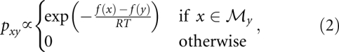 |
where  is the neighborhood of y, i.e., the set of conformations that can be generated from y by applying a move m ∈ M.
As demonstrated in Wolfinger et al. (2004), one can approximate this dynamics by a dynamics on the set of macrostates provided one can argue that the process is approximately equilibrated within each class of Π. A slightly cruder, but computationally much more efficient approximation entails an Arrhenius ansatz using the barrier tree to estimate the activation energies. For any two local minima  we define their transition state energy
  as the energy level at which their associated macrostates merge in the barrier tree, i.e.,
Note that this expression coincides with the more “usual” definition of the barrier height as the minimum of the maximal height of paths connecting and (see, e.g., Nemoto 1988). The advantage of Equation 3 is that it emphasizes that the saddle height can be computed as the merging of cycles within a flooding algorithm (Flamm et al. 2000) instead of the (algorithmically infeasible) optimization over all paths.
Transition rates between macrostates, represented here by the local minima that define them, are then given by the Arrhenius law
 |
where A is a normalization constant. For further details we refer to Wolfinger et al. (2004).
Barmaps
Given a landscape we now may ask how the folding behavior changes if we perturb the landscape. Such perturbations can take a wide variety of forms:
 remains the same, only the energy function is perturbed, f → g. This is the case, e.g., when the temperature or ionic strength of the system is changed.
(X,f) remains the same, but the move set changes
 . This case is of interest when one is interested in the sensitivity of folding kinetics to changes in the underlying mechanistic models, e.g., to assess the impact of shift moves (Wuchty et al. 1998)
X,f, and
 change systematically. Examples are cotranscriptional folding or for experimental manipulations such as pulling an RNA molecule through a pore.
Our goal is to consider these types of changes in a coherent way in the framework of barrier trees. This will allow us to approximate the folding dynamics in time-variable landscapes of various types. Since we model the dynamics at the level of macrostates, we need to investigate how the perturbation of the landscape translates into changes of the barrier trees and their associated macrostates. In other words, we need to construct a map  from the macrostates of to the macrostates of
  .
.
From a mathematical point of view, we first of all need a map  that specifies how the perturbation affects an individual conformation x before it “relaxes” in the modified landscapes. In the first two cases, this map is trivial: It coincides with the identity map,
  , since the set of conformations does not change.
In the case of cotranscriptional folding it is also quite simple: When the next nucleotide is appended to a growing chain, it initially does not interact with the already folded “head” of the molecules, so that x′ is x with an unpaired base appended.
The situation is a bit more complex in scenarios such as translocation of macromolecules through pores, or other mechanical constraints. In the pore case, suppose the RNA moves through the pore from 3′ to 5′, and k is the position directly 5′ of the pore. Then, the RNA structure is composed of two independently folding parts x[1…k] and  , while the interval
  is located within the pore, and hence, inaccessible to base pairing. In the next step, the 5′ part is x[1…k − 1]; if k was paired, the base pair (j,k) now has been opened because nucleotide k is now covered by the pore. The other part is
  , where the first position
  emerges unpaired from the pore. Note that in the pore case, the gradient descent operator γ also needs to be restricted to producing independent structures on both sides of the pore. For simplicity, assume a constant speed of translocation rather than explicitly modeling a pulling force; in the latter case we would have to include the distortion of the energy landscape caused by the pulling force (see, e.g., Gerland et al. 2004).
In the landscape we have again well-defined gradient basins by means of the steepest descent operator γ′ on this landscape. The concatenation  thus maps every local minimum of to a local minimum of the perturbed by first reinterpreting z in the new context and then relaxing it to the local minimum of the associated basin. It therefore implies the desired mapping β that maps macrostates of to the macrostates of . In other words, β maps the leaves of the barrier tree to the leaves of the barrier tree
  . We thus refer to β as the barrier tree map, or barmap for short, Figure 3.
FIGURE 3.

Schematic of the barmap between two consecutive landscapes. Three types of events may occur: (1) two (here, the two left-most minima) local minima in  merge into one; (2) a new minimum (marked by *) appears in
  ; and (3) one-to-one correspondence between minima (as for the right-most minimum here).
Note that, in general, the barmap is neither injective nor surjective: There may be local minima in that are not the image of any local minimum of , while multiple local minima of may be merged into a single minimum of .
Kinetics on time-variable landscapes
The formalism developed in the previous subsections can be exploited to approximate RNA (re)folding kinetics on time-variable landscapes. The idea is to first determine a sequence of barrier trees  together with barmaps
  . These data have to be determined only once. We are then free to choose a sequence {Tk} of time points at which the system proceeds from to
  . This allows us to explore the effects of variations in the speed of transcription, the rate temperature changes, or the pulling force in a manner that is independent of the computationally expensive analysis of the energy landscapes.
Denote by  the initial condition, i.e., the population densities in macrostate on barrier tree
  at time 0. The population density on just before the transition to is
  . The initial condition on the next barrier tree Bk+1 is obtained by collecting for each macrostate the population densities of all those macrostates of the previous barrier tree that map to under the barmap βk. In symbols:
Within the time interval [Tk,Tk+1] we simply have to solve the master equation
with  and the initial conditions described above. Note that the transition matrix
  is by assumption independent of time for each fixed barrier tree. Thus, the expensive part of solving the Master equation, namely the diagonalization of P, is also independent of the time intervals, and thus has to be performed only once for each barrier tree. The computational effort for the diagonalization grows as
  , where N is the number of macrostates. For our applications, N is typically around 1000, allowing diagonalization within a couple of seconds. After these preparatory computations have been performed, the population dynamics for a given schedule {Tk} can be evaluated with a few matrix and vector multiplications. This sets the stage for an in-depth analysis of the interplay of folding dynamics and changes in the energy landscapes without substantial computational costs.
RESULTS
The BarMap software
The BarMap software is implemented as a combination of C programs and Perl scripts that form a pipeline for simulating folding time-dependent energy landscapes. In the first step of the pipeline, all low-energy structures of a landscape are computed using RNAsubopt from the Vienna RNA package. Subsequently, they are analyzed by the barriers program (Flamm et al. 2000). This is done separately for each landscape in the time series and yields both a barrier tree and a matrix of effective transition rates. The bar_map Perl program then computes the barmap β between consecutive barrier trees. Folding dynamics on each landscape are computed by the treekin program (Wolfinger et al. 2004). The final population on the landscape at time step k − 1 is mapped to the the initial population on the landscape at time step k using the barmap βk. A helper Perl script, barmap_simulator, is available that automatically generates the necessary treekin command lines. In order to plot folding dynamics as shown in Figures 4 and 5 the treekin trajectory for the time intervals in which the landscapes is fixed are stitched together using the barmaps βk, k ≥ 1. This is accomplished by the final bmjoin script. An accompanying visualization tool, BarMapViz (Heine et al. 2006) can be used to create movies of barrier tree sequences, facilitating the analysis of the landscape features that are responsible for particular kinetic effects.
FIGURE 4.

Hysteresis effects in an thermosensitive RNA. In this example, the temperature cycles 10 times from 10 to 59°C, as shown at top. The second panel shows a nearly adiabatic temperature change (1015 time units per cycle), such that the system is always near equilibrium. Panels 3 to 5 show increasingly faster temperature cycles, with 105, 104, and 103 time units per cycle. The RNA has different optimal conformations at 10°C (solid black) and 59°C (dashed black), respectively. At high temperatures, furthermore, the minimum energy structure is nearly degenerate, so that an alternative structure (dotted gray) is populated in panels 2 and 3. For the very fast temperature cycle (bottom), the RNA is trapped in the low-temperature structure. Here, the only structural change is the opening of a GU:GU stack at high temperatures (gray area in structure drawing).
FIGURE 5.

Cotranscriptional folding of the E. coli leader RNA of the tRNAphe synthetase operon for two different transcription speeds. For slow transcription (top) the completely transcribed chain shows a nearly zero density for the terminator structure (solid black line), and transcription of the full-length operon proceeds. For fast transcription, most of the fully elongated molecules form the terminator structure (dashed line). Thermodynamic equilibrium is reached only on very long (>1010) time scales.
Source code for the barriers and treekin programs, as well as the bar_map, barmap_simulator, and bmjoin Perl programs, is available from http://www.tbi.univie.ac.at/RNA/Barriers/.
Application 1: A RNA thermometer
Figure 4 shows the refolding dynamics of an artificial RNA thermometer when cycling between a high and low temperature regime. The sequence was designed using the RNA switch designer described by Flamm et al. (2001), taking into account the sequence and structure constraints listed in Waldminghaus et al. (2008). This study demonstrated that in silico design with subsequent in vivo fine-tuning can produce temperature-controlled RNA elements with efficiencies comparable to their natural counterparts. For very slow temperature cycles (top), the molecule behaves adiabatically, effectively reaching thermodynamic equilibrium at each time step. The dynamics is therefore determined entirely by the barrier trees and the connecting barmaps. For intermediate cycling frequencies (104−105 time units per cycle), the system prefers the high-temperature structure. The relaxation time increases with cycling frequency. At even faster cycles, the system is trapped close to the (low temperature) starting conformation, since it does not have sufficient time to refold before the temperature drops again.
Application 2: Cotranscriptional folding
Under cellular conditions, RNA molecules start to fold before transcription is completed. This phenomenon is exploited by many bacteria to regulate the expression of amino acid biosynthesis genes (Yanofsky 2000; Vitreschak et al. 2004; Merino et al. 2008). This RNA-based regulatory strategy by premature termination of transcription, often called transcription attenuation (Henkin and Yanofsky 2002), relies on the selective formation of either of two mutually exclusive RNA secondary structures (the anti-terminator and the terminator) in the nascent transcript. The terminator structure causes premature termination of transcription.
We investigated the cotranscriptional folding dynamics of the leader RNA of the phenylalanine tRNA synthetase operon from E. coli (Fayat et al. 1983) under different transcription speeds, see Figure 5. For slow transcription, when the full-length chain is produced after ∼105 arbitrary time units, the anti-terminator structure is formed (Fig. 5, top left panel). In contrast, under fast transcription conditions (transcription completed already after ∼104 arbitrary time units), the terminator structure is formed (Fig. 5, bottom left panel). Since transcription attenuation operates far from the thermodynamic equilibrium, the kinetic competition between two small stem–loop structures (see blow-up panels on the right) decides whether the full-length leader RNA will eventually end up in the terminator or the anti-terminator structure. This competition early in the folding process is highly sensitive to the speed of transcription. Note, that for very long folding times (∼1011) both cotranscriptional folding scenarios converge, as expected, to the thermodynamic equilibrium, which is dominated by the more stable terminator structure.
In vivo, elongation speed is not constant, but influenced by site-specific pausing of the RNA polymerase and interactions of the nascent RNA with proteins (Pan and Sosnick 2006). The effect of pause sites can easily be included in our approach. One simply needs to specify an appropriate elongation speed profile, i.e., an explicit list of time-points {Tk} for the transitions from one landscape to the next.
Application 3: Refolding during pore translocation
The transport of biopolymers through narrow pores is a fundamental process in life that is often coupled to the dynamics of biopolymer structure formation, e.g., the base-pair unfolding and folding dynamics while an mRNA passes through the ribosome during translation. Translocation of polymers is hindered by an entropic barrier, since the narrow confinement of the pore effectively separates the biopolymer into two independent sections, resulting in a reduction of the chain entropy and, hence, an increase of the free energy of the chain (Muthukumar 2007).
For structured nucleic acids, further kinetic barriers arise, since the molecule has to locally unfold while passing through the pore Bundschuh and Gerland 2005; McCauley et al. 2009). In recent years, the single-molecule techniques of driving biopolymers through nano-pores using electric fields have been used to explore experimentally the structural and dynamic properties of nucleic acids (Vercoutere et al. 2001; Sauer-Budge et al. 2003; Mathé et al. 2004; Dudko et al. 2007).
We model the effect of the pore by allowing only secondary structures that are unpaired within the pore and contain no base pairs crossing from one side of the pore to the other. Figure 6 shows the resulting translocation dynamics for an artificial RNA sequence. In this example we use a slow translocation rate that allows the base-pairing pattern on both sides of the pore to almost equilibrate.
FIGURE 6.

Translocation of the artificial RNA sequence UUUUAGCCUCUUUGAGGUCGCCAUGCGAUUUUUUUU through a pore with a length of 5 nt. The RNA enters the pore with its 3′ end. As more and more of the minimum free energy (MFE) structure (black) is occluded by the pore, the RNA refolds into alternative structures (dotted and dashed). At the mid point, the most likely structure is the open chain (solid gray). Note how the probability of the MFE almost reaches 100% at t ≈ 290 when the structure is fully formed but alternative structures are inhibited by the pore.
DISCUSSION
We have introduced here a very generic approach to investigate in detail the dynamic aspects of RNA folding in scenarios that involve external stimuli and/or changes of environment. By separating changes in the energy landscapes from the dynamics on these landscapes it becomes possible to avoid the extensive simulation of individual trajectories altogether. The examples described in the previous section highlight the major advantage of the BarMap approach: Each energy landscape and its barrier tree and all of the barmaps between adjacent landscapes need to be computed only once. The transition rate matrices between macrostates within a landscape also have to be computed and diagonalized only once. The systematic exploration of the effects of different rates of change in the environment can thus be conducted very efficiently without the need to recompute any landscape-specific data. Time series of population densities, in fact, can be obtained using a few simple matrix and vector multiplications. The BarMap approach is thus particularly suitable to study the subtle kinetic effect that arises from the intricate interplay of different time scales.
MATERIALS AND METHODS
RNA folding
All structure predictions were performed with the Vienna RNA package (Hofacker et al. 1994) version 1.8.3, using the Turner energy parameters as described in Mathews et al. (1999).
Visualization of barrier tree series
In order to gain a thorough understanding of the effects of changes in the landscape, one needs to comprehend how these changes affect the corresponding barrier trees. To this end, we have developed the BarMapVis tool to create an animation of a sequence of barrier trees and the leaf mappings between adjacent trees (Heine et al. 2006). In brief, BarMapVis is based on the foresight layout with tolerance algorithm (Diehl and Görg 2002), a very general attempt to solve any offline dynamic graph drawing problem. First, a directed acyclic supergraph G* is constructed that contains all barrier trees as subgraphs and reflects the topological properties of all energy landscapes. The supergraph G* is then laid out in the plane using a modified version of dot (Gansner et al. 1993). Finally, the layout of the subgraphs is determined by using the layout of the supergraph as a template following static drawing aesthetic criteria in a way that approximately preserves the mental map (Misue et al. 1995) between consecutive barrier trees.
Animations showing the sequence of barrier trees generated by BarMapVis for each of the three examples from the Results section can be found in the web supplement.
SUPPLEMENTAL MATERIAL
Machine readable files of the input sequences, barrier trees, and BarMapVis movies can be downloaded from http://www.tbi.univie.ac.at/papers/SUPPLEMENTS/BarMap/. The barmap software can be downloaded from the barriers website http://www.tbi.univie.ac.at/RNA/Barriers/.
ACKNOWLEDGMENTS
We thank Konstantin Klemm for stimulating discussions. This work has been funded in part by the Austrian GEN-AU projects “bioinformatics integration network III” and “regulatory noncoding RNA,” the German DFG Bioinformatics Initiative BIZ-6/1-2, and the COST Action CM0703 “Systems Chemistry.”
Footnotes
Article published online ahead of print. Article and publication date are at http://www.rnajournal.org/cgi/doi/10.1261/rna.2093310.
REFERENCES
- Abrahams JP, van den Berg M, van Batenburg E, Pleij C 1990. Prediction of RNA secondary structure, including pseudoknotting, by computer simulation. Nucleic Acids Res 18: 3035–3044 [DOI] [PMC free article] [PubMed] [Google Scholar]
- Baumstark T, Schroder AR, Riesner D 1997. Viroid processing: Switch from cleavage to ligation is driven by a change from a tetraloop to a loop E conformation. EMBO J 16: 599–610 [DOI] [PMC free article] [PubMed] [Google Scholar]
- Becker OM, Karplus M 1997. The topology of multidimensional potential energy surfaces: Theory and application to peptide structure and kinetics. J Chem Phys 106: 1495–1517 [Google Scholar]
- Bundschuh R, Gerland U 2005. Coupled dynamics of RNA folding and nanopore translocation. Phys Rev Lett 95: 208104/1–208104/4 doi: 10.1103/PhysRevLett.95.208104 [DOI] [PubMed] [Google Scholar]
- Clote P 2005. An efficient algorithm to compute the landscape of locally optimal RNA secondary structures with respect to the Nussinov–Jacobson energy model. J Comput Biol 12: 83–101 [DOI] [PubMed] [Google Scholar]
- Diehl S, Görg C 2002. Graphs, they are changing—dynamic graph drawing for a sequence of graphs. In Proceedings of 10th international symposium on graph drawing (ed. Goodrich MT, Kobourov SG), no. 2528, pages 23–31 Springer, Heidelberg, Germany [Google Scholar]
- Doye JP, Miller MA, Welsh DJ 1999. Evolution of the potential energy surface with size for Lennard-Jones clusters. J Chem Phys 111: 8417–8429 [Google Scholar]
- Dudko OK, Mathé J, Szabo A, Meller A, Hummer G 2007. Extracting kinetics from single-molecule force spectroscopy: Nanopore unzipping of DNA hairpins. Biophys J 92: 4188–4195 [DOI] [PMC free article] [PubMed] [Google Scholar]
- Fayat G, Mayaux JF, Sacerdot C, Fromant M, Springer M, Grunberg-Manago M, Blanquet S 1983. Escherichia coli phenylalanyl-tRNA synthetase operon region. Evidence for an attenuation mechanism. Identification of the gene for the ribosomal protein L20. J Mol Biol 171: 239–261 [DOI] [PubMed] [Google Scholar]
- Flamm C, Hofacker IL 2008. Beyond energy minimization: Approaches to the kinetic folding of RNA. Monatsh Chem 139: 447–457 [Google Scholar]
- Flamm C, Fontana W, Hofacker I, Schuster P 2000. RNA folding kinetics at elementary step resolution. RNA 6: 325–338 [DOI] [PMC free article] [PubMed] [Google Scholar]
- Flamm C, Hofacker IL, Maurer-Stroh S, Stadler PF, Zehl M 2001. Design of multistable RNA molecules. RNA 7: 254–265 [DOI] [PMC free article] [PubMed] [Google Scholar]
- Flamm C, Hofacker IL, Stadler PF, Wolfinger MT 2002. Barrier trees of degenerate landscapes. Z Phys Chem 216: 155–173 [Google Scholar]
- Gansner ER, Koutsofios E, North SC, Vo KP 1993. A technique for drawing directed graphs. IEEE Trans Softw Eng 19: 214–230 [Google Scholar]
- Garstecki P, Hoang TX, Cieplak M 1999. Energy landscapes, supergraphs, and ‘folding funnels’ in spin systems. Phys Rev E Stat Phys Plasmas Fluids Relat Interdiscip Topics 60: 3219–3226 [DOI] [PubMed] [Google Scholar]
- Gerdes K, Wagner GH 2007. RNA antitoxins. Curr Opin Microbiol 10: 117–124 [DOI] [PubMed] [Google Scholar]
- Gerland U, Bundschuh R, Hwa T 2004. Translocation of structured polynucleotides through nanopores. Phys Biol 1: 19–26 [DOI] [PubMed] [Google Scholar]
- Gollnick P, Babitzke P, Antson A, Yanofsky C 2005. Complexity in regulation of tryptophan biosynthesis in Bacillus subtilis. Annu Rev Genet 39: 47–68 [DOI] [PubMed] [Google Scholar]
- Gultyaev AP 1991. The computer simulation of RNA folding involving pseudoknot formation. Nucleic Acids Res 19: 2489–2493 [DOI] [PMC free article] [PubMed] [Google Scholar]
- Heidrich D, Kliesch W, Quapp W 1991. Properties of chemically interesting potential energy surfaces, In Lecture notes in chemistry, vol. 56 Springer, Berlin, Germany [Google Scholar]
- Heine C, Scheuermann G, Flamm C, Hofacker IL, Stadler PF 2006. Visualization of barrier tree sequences. IEEE Trans. Vis. Comp. Graphics 12: 781–788 [DOI] [PubMed] [Google Scholar]
- Henkin TM, Yanofsky C 2002. Regulation by transcription attenuation in bacteria: How RNA provides instructions for transcription termination/antitermination decisions. Bioessays 24: 700–707 [DOI] [PubMed] [Google Scholar]
- Hofacker IL, Fontana W, Stadler PF, Bonhoeffer LS, Tacker M, Schuster P 1994. Fast folding and comparison of RNA secondary structures. Monatsh Chem 125: 167–188 [Google Scholar]
- Hofacker IL, Schuster P, Stadler PF 1998. Combinatorics of RNA secondary structures. Discrete Appl Math 88: 207–237 [Google Scholar]
- Klinkert B, Narberhaus F 2009. Microbial thermosensors. Cell Mol Life Sci 66: 2661–2676 [DOI] [PMC free article] [PubMed] [Google Scholar]
- Klotz T, Kobe S 1994. ‘Valley structures’ in the phase space of a finite 3D Ising spin glass with ±i interactions. J Phys Math Gen 27: L95–L100 [Google Scholar]
- Martinez HM 1984. An RNA folding rule. Nucleic Acids Res 12: 323–335 [DOI] [PMC free article] [PubMed] [Google Scholar]
- Mathé J, Visram H, Viasnoff V, Rabin Y, Meller A 2004. Nanopore unzipping of individual DNA hairpin molecules. Biophys J 87: 3205–3212 [DOI] [PMC free article] [PubMed] [Google Scholar]
- Mathews D, Sabina J, Zuker M, Turner H 1999. Expanded sequence dependence of thermodynamic parameters provides robust prediction of RNA secondary structure. J Mol Biol 288: 911–940 [DOI] [PubMed] [Google Scholar]
- McCauley M, Forties R, Gerland U, Bundschuh R 2009. Anomalous scaling in nanopore translocation of structured heteropolymers. Phys Biol 6: 036006 doi: 10.1088/1478-3975/6/3/036006 [DOI] [PubMed] [Google Scholar]
- Merino E, Jensen RA, Yanofsky C 2008. Evolution of bacterial trp operons and their regulation. Curr Opin Microbiol 11: 78–86 [DOI] [PMC free article] [PubMed] [Google Scholar]
- Mezey PG 1987. Potential energy hypersurfaces Elsevier, Amsterdam, The Netherlands [Google Scholar]
- Mironov AA, Dyakonova LP, Kister AE 1985. A kinetic approach to the prediction of RNA secondary structures. J Biomol Struct Dyn 2: 953–962 [DOI] [PubMed] [Google Scholar]
- Misue K, Eades P, Lai W, Sugiyama K 1995. Layout adjustment and the mental map. J Vis Lang Comput 6: 183–210 [Google Scholar]
- Muthukumar M 2007. Mechanism of DNA transport through pores. Annu Rev Biophys Biomol Struct 36: 435–450 [DOI] [PubMed] [Google Scholar]
- Narberhaus F, Waldminghaus T, Chowdhury S 2006. RNA thermometers. FEMS Microbiol Rev 30: 3–16 [DOI] [PubMed] [Google Scholar]
- Nemoto K 1988. Metastable states of the SK spin glass model. J Phys A 21: L287–L294 [Google Scholar]
- Pan T, Sosnick T 2006. RNA folding during transcription. Annu Rev Biophys Biomol Struct 35: 161–175 [DOI] [PubMed] [Google Scholar]
- Perrotta AT, Been MD 1998. A toggle duplex in hepatitis delta virus self-cleaving RNA that stabilizes an inactive and a salt-dependent pro-active ribozyme conformation. J Mol Biol 279: 361–373 [DOI] [PubMed] [Google Scholar]
- Rapaport DC 2004. The art of molecular dynamics simulation Cambridge University Press, 2nd ed Cambridge, UK [Google Scholar]
- Reidys CM, Stadler PF 2002. Combinatorial landscapes. SIAM Rev 44: 3–54 [Google Scholar]
- Sauer-Budge AF, Nyamwanda JA, Lubensky DK, Branton D 2003. Unzipping kinetics of double-stranded DNA in a nanopore. Phys Rev Lett 90: doi: 10.1103/PhysRevLett.90.238101 [DOI] [PubMed] [Google Scholar]
- Schultes EA, Bartel DP 2000. One sequence, two ribozymes: Implications for the emergence of new ribozyme folds. Science 289: 448–452 [DOI] [PubMed] [Google Scholar]
- Tacker M, Fontana W, Stadler PF, Schuster P 1994. Statistics of RNA melting kinetics. Eur Biophys J 23: 29–38 [DOI] [PubMed] [Google Scholar]
- Tang X, Thomas S, Tapia L, Giedroc DP, Amato NM 2008. Simulating RNA folding kinetics on approximated energy landscapes. J Mol Biol 381: 1055–1067 [DOI] [PubMed] [Google Scholar]
- Thirumalai D, Lee N, Woodson SA, Klimov DK 2001. Early events in RNA folding. Annu Rev Phys Chem 52: 751–762 [DOI] [PubMed] [Google Scholar]
- Vercoutere W, Winters-Hilt S, Olsen H, Deamer D, Haussler D, Mar Akeson M 2001. Rapid discrimination among individual DNA hairpin molecules at single-nucleotide resolution using an ion channel. Nat Biotechnol 19: 248–252 [DOI] [PubMed] [Google Scholar]
- Vitreschak AG, Lyubetskaya EV, Shirshin MA, Gelfand MS, Lyubetsky VA 2004. Attenuation regulation of amino acid biosynthetic operons in proteobacteria: Comparative genomics analysis. FEMS Microbiol Lett 234: 357–370 [DOI] [PubMed] [Google Scholar]
- Waldminghaus T, Kortmann J, Gesing S, Narberhaus F 2008. Generation of synthetic RNA-based thermosensors. Biol Chem 389: 1319–1326 [DOI] [PubMed] [Google Scholar]
- Wales DJ, Miller MA, Walsh TR 1998. Archetypal energy landscapes. Nature 394: 758–760 [Google Scholar]
- Wolfinger MT, Svrcek-Seiler WA, Flamm C, Hofacker IL, Stadler PF 2004. Efficient computation of RNA folding dynamics. J Phys Math Gen 37: 4731–4741 [Google Scholar]
- Wolfinger MT, Will S, Hofacker IL, Backofen R, Stadler PF 2006. Exploring the lower part of discrete polymer model energy landscapes. Europhys Lett 74: 726–732 [Google Scholar]
- Wuchty S, Fontana W, Hofacker IL, Schuster P 1998. Complete suboptimal folding of RNA and the stability of secondary structure. Biopolymers 49: 145–165 [DOI] [PubMed] [Google Scholar]
- Yanofsky C 2000. Transcription attenuation: Once viewed as a novel regulatory strategy. J Bacteriol 182: 1–8 [DOI] [PMC free article] [PubMed] [Google Scholar]