A fast, angle-dependent, analytical model of CsI detector response for optimization of 3D x-ray breast imaging systems

Abstract

Purpose: Accurate models of detector blur are crucial for performing meaningful optimizations of three-dimensional (3D) x-ray breast imaging systems as well as for developing reconstruction algorithms that faithfully reproduce the imaged object anatomy. So far, x-ray detector blur has either been ignored or modeled as a shift-invariant symmetric function for these applications. The recent development of a Monte Carlo simulation package called MANTIS has allowed detailed modeling of these detector blur functions and demonstrated the magnitude of the anisotropy for both tomosynthesis and breast CT imaging systems. Despite the detailed results that MANTIS produces, the long simulation times required make inclusion of these results impractical in rigorous optimization and reconstruction algorithms. As a result, there is a need for detector blur models that can be rapidly generated.

Methods: In this study, the authors have derived an analytical model for deterministic detector blur functions, referred to here as point response functions (PRFs), of columnar CsI phosphor screens. The analytical model is x-ray energy and incidence angle dependent and draws on results from MANTIS to indirectly include complicated interactions that are not explicitly included in the mathematical model. Once the mathematical expression is derived, values of the coefficients are determined by a two-dimensional (2D) fit to MANTIS-generated results based on a figure-of-merit (FOM) that measures the normalized differences between the MANTIS and analytical model results averaged over a region of interest. A smaller FOM indicates a better fit. This analysis was performed for a monochromatic x-ray energy of 25 keV, a CsI scintillator thickness of 150 μm, and four incidence angles (0°, 15°, 30°, and 45°).

Results: The FOMs comparing the analytical model to MANTIS for these parameters were 0.1951±0.0011, 0.1915±0.0014, 0.2266±0.0021, and 0.2416±0.0074 for 0°, 15°, 30°, and 45°, respectively. As a comparison, the same FOMs comparing MANTIS to 2D symmetric Gaussian fits to the zero-angle PRF were 0.6234±0.0020, 0.9058±0.0029, 1.491±0.012, and 2.757±0.039 for the same set of incidence angles. Therefore, the analytical model matches MANTIS results much better than a 2D symmetric Gaussian function. A comparison was also made against experimental data for a 170 μm thick CsI screen and an x-ray energy of 25.6 keV. The corresponding FOMs were 0.3457±0.0036, 0.3281±0.0057, 0.3422±0.0023, and 0.3677±0.0041 for 0°, 15°, 30°, and 45°, respectively. In a previous study, FOMs comparing the same experimental data to MANTIS PRFs were found to be 0.2944±0.0027, 0.2387±0.0039, 0.2816±0.0025, and 0.2665±0.0032 for the same set of incidence angles.

Conclusions: The two sets of derived FOMs, comparing MANTIS-generated PRFs and experimental data to the analytical model, demonstrate that the analytical model is able to reproduce experimental data with a FOM of less than two times that comparing MANTIS and experimental data. This performance is achieved in less than one millionth the computation time required to generate a comparable PRF with MANTIS. Such small computation times will allow for the inclusion of detailed detector physics in rigorous optimization and reconstruction algorithms for 3D x-ray breast imaging systems.

INTRODUCTION

Optimization of three-dimensional (3D) breast x-ray imaging systems and 3D image reconstruction methods rely on assumptions about detector performance. The deterministic blur introduced by the detector can be quantified by the point response function (PRF), which is the resultant image of an infinitely thin x-ray pencil beam. The current approach to modeling detector performance assumes that the PRF has a symmetric shape that is invariant over the detector area.^{1, 2} In some cases, detector blur is ignored altogether.^{3, 4} However, recent studies^{5, 6, 7} have demonstrated that there are large variations in the PRF across the detector face and that it can be highly asymmetric for large incidence angles. A recent study measured the MTF of an experimental benchtop tomosynthesis system with a flat panel indirect detector as used in a GE Senographe 2000D system.⁷ The source-detector distance was 112 cm and the object-detector distance was 5 cm. X-ray incidence angles of 0°, 10°, 20°, 30°, 40°, and 50° were investigated for two different x-ray spectra (26 kVp Mo∕Mo and 40 kVp Rh∕Al with an additional 1 mm Al filter). A decreasing MTF with incidence angle demonstrated that the detector performance deteriorates significantly as the incidence angle increases.

In addition, the recent development of a detailed Monte Carlo simulation code [MANTIS (Refs. ^{8, 9})] (a current version of the code, tutorials, and examples are available from ftp://150.148.3.14/mantis) for studying the imaging performance of modern CsI columnar phosphor screens has demonstrated similar variations in the PRF over the detector face for both breast tomosynthesis and CT-like geometries. Badano et al.⁵ investigated a tomosynthesis geometry with a source-to-detector distance of 60 cm and an angle between the chest wall and the edge of the x-ray beam of 11.3°. The detector was a small mammography detector with a size of 24×12 cm² and a phosphor screen thickness of 150 μm. The x-ray tube was allowed to rotate on an arc centered about the detector plane with an angular range of ±20°. Three different x-ray spectra were considered (Mo∕Mo at 28 kVp, Rh∕Rh at 28 kVp, and W∕Al at 42 kVp) as well as three different breast thicknesses (3, 4, and 6 cm). This geometry resulted in x rays entering the phosphor screen at angles of up to 45°. The PRFs showed significant anisotropy and increased blurring as compared to normal x-ray incidence. In another paper, simulations were carried out for a breast CT system.⁶ This system had a source-to-isocenter distance of 44 cm, a source-to-detector distance of 88 cm, and a 30×40 cm² detector with a 600 μm thick phosphor screen, with x-ray energies of 30–70 keV. Increases in blur with respect to normal x-ray incidence were measured by performing a two-dimensional (2D) Gaussian fit to the PRFs and dividing the major axis of the fitted Gaussian with the major axis of the fitted Gaussian at zero degree incidence. For the investigated x-ray energies and incidence angles, the measured blur values were as high as 1.86. Also, the maximum aspect ratios of the PRFs ranged from 1.14 to 2.53, depending on the contour level for the height of the PRF chosen for the analysis.

Unfortunately, because of the long simulation times required for the detailed MANTIS code (approximately 200 h on a single 3 GHz CPU for a PRF with 500 000 primary x rays), accurate PRFs have yet to be incorporated into optimization and reconstruction schemes. In this work, we have developed a closed-form, deterministic, analytical model that approximates the detailed Monte Carlo simulations in less than one millionth of the computation time (about 0.1 s). The model describes the depth-dependent deterministic response of the detector. In addition, our model could be used to simulate the noise component present in indirect detectors due to variations in the optical processes. The analytical model has been developed for a single CsI phosphor thickness (150 μm), x-ray energy (25 keV), and four incidence angles (0°, 15°, 30°, and 45°). Future expansion of the model to a larger range of parameters will allow for rapid, on-the-fly generation of PRFs that will enable the inclusion of realistic detector performances in system optimization and reconstruction.

In Sec. 2 the detailed derivation of the PRF model is presented. Calculation of the best fit coefficient values as well as a quantitative comparison with MANTIS-generated PRFs is discussed in Sec. 3. Section 4 gives the results of a comparison of the analytical model with experimental data. Finally, conclusions are provided in Sec. 5.

THE MODEL

The objective of this analytical model is to produce a deterministic PRF for a given set of system parameters. Therefore, all incident x rays are specified to arrive at the same location (x,y,z)=(0,0,0) and with the same incidence angle (θ,ϕ). Additionally, we assume a monochromatic incident beam with energy E. The general approach used in this model can be broken down into two major steps. In the first step (discussed in the remainder of this section), we model the physics of the interaction between the incoming x-ray beam and the CsI crystal. This analysis produces an analytical expression that describes the shape of a PRF for a given set of input parameters. In the second step (see Sec. 3), the free parameters in the analytical expression are adjusted by fitting that expression to PRFs produced using MANTIS.

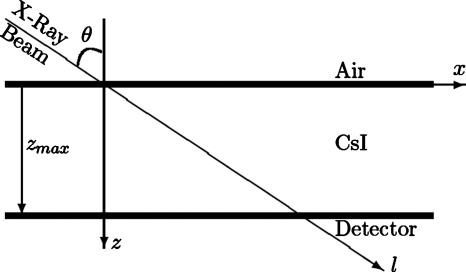
In the first step, we have ignored the columnar structure of the CsI crystal in the mathematical formulation and made the assumption that it is a homogeneous, solid slab. Although the effects of columnar structure are not explicitly included in the mathematics, they are indirectly included by using MANTIS data as a guide to choosing the functional forms of the relevant physical properties. In addition, the second step incorporates the columnar structure and other secondary effects by adjusting the free parameters in the model based on MANTIS data. Figure 1 shows a schematic of the model geometry and coordinate system, while Table 1 gives definitions for variables used in the derivation of the model.

Figure 1.

Schematic of model geometry and coordinate system. The view is a vertical cut through the CsI crystal looking from the side with the air interface on the top and the detector layer at the bottom of the schematic. The infinitely thin incident x-ray beam enters at an angle of 90° minus θ from the x axis (ϕ, 90° minus the angle between the x-ray beam and the y axis, is assumed to be zero in this diagram). The y axis is going out of the page in this view.

Table 1.

Definition of model variables.

Symbol	Definition
(x,y,z)	X ray interaction location (z=depth in crystal)(0,0,0)=x-ray crystal entrance
l	Position along x ray travel direction(=0 at x-ray crystal entrance) $=\sqrt{x^2+y^2+z^2}$
θ	90° minus the angle between the l and x axes(sin θ=x∕l)
ϕ	90° minus the angle between the l and y axes(sin ϕ=y∕l)
zmax	Thickness of crystal
μpe(E)	Photoelectric attenuation coefficient of CsI (cm−1)
μtot(E)	Total attenuation coefficient of CsI (cm−1)
E	Energy of incident x rays (keV)
No	No. of incident x ray photons
γ	X ray to optical-photon gain factor (keV−1)

Four separate effects in the x-ray detection process are modeled in the first step of our approach. The first is the depth-dependent absorption of the incident x rays. The second is the conversion of the absorbed x rays into the emitted optical photons by the CsI crystal. The third is the self-absorption of the emitted optical photons in the CsI crystal and the absorption of the photodiode layer. Finally, the fourth is the depth-dependent spread of the optical photons collected at the exit plane of the crystal. Subsections 2A, 2B, 2C, 2D, 2E describe each of these effects in detail and then integrate the final depth-dependent model over the crystal thickness to get an analytical expression for the overall PRF.

Depth-dependent absorption of incident x rays

Gallas et al.¹⁰ derived a model for image formation with indirect x-ray powder-phosphor based detectors. Following their analysis, the rate at which x-ray photons interact with the crystal as a function of crystal depth is given by

$$N_i\left(z,\theta ,\varphi ,E\right)=N_o{\eta }_{\text{x-ray}}\left(z,\theta ,\varphi ,E\right),$$ (1)

where η_x-ray(z,θ,ϕ,E) is the x-ray interaction probability for a given depth.

Here, we restrict our analysis to consider only x rays that interact with the crystal via the photoelectric effect to produce an optical-photon shower that can subsequently be detected with a photodiode array. Therefore, we can further write

$$N_{\text{pe}}\left(z,\theta ,\varphi ,E\right)=\frac{{\mu }_{\text{pe}}\left(E\right)}{{\mu }_{\text{tot}}\left(E\right)}{N}_i\left(z,\theta ,\varphi ,E\right)$$ (2)

as the number of photons that interact with the CsI crystal to produce an optical-photon shower, where μ_pe(E) is the photoelectric attenuation coefficient of the crystal. Figure 2 shows the importance of different interaction types at energies applicable to breast imaging. The total mass attenuation coefficient as well as the contributions to the total mass attenuation coefficient due to the photoelectric, Rayleigh, and Compton effects are shown as a function of energy in the range of 5–100 keV. These values were calculated using pure CsI in the Monte Carlo simulation package PENELOPE.^{11, 12} The photoelectric effect is the dominant interaction type for this energy range and constitutes 89.3%–99.4% of the total mass attenuation coefficient. Note that the fitting algorithm discussed in Sec. 3 should help compensate for the Compton and Rayleigh contributions to the detected signal that are not included in the model.

Figure 2.

Mass attenuation coefficient as a function of energy for CsI as simulated in PENELOPE. The photoelectric, Rayleigh, Compton, and total mass attenuation coefficients are shown. The photoelectric effect is the dominant interaction over the energy range of 5–100 keV.

To calculate η_x-ray(z,θ,ϕ,E) as a function of depth, we can start by writing from first principles the same expression as a function of position along the travel direction

$${\eta }_{\text{x-ray}}\left(l,\theta ,\varphi ,E\right)={\mu }_{\text{tot}}\left(E\right)\text{exp}\left(-{\mu }_{\text{tot}}\left(E\right)l\right).$$ (3)

In order to write this as a function of the crystal depth (z), we can relate l and z with the following equation:

$$l=\frac{z}{\sqrt{{\text{cos}}^2\theta -{\text{sin}}^2\varphi }}$$ (4)

and replace l by z in Eq. 3 to get

$${\eta }_{\text{x-ray}}\left(z,\theta ,\varphi ,E\right)={\mu }_{\text{tot}}\left(E\right)\text{exp}\left(-\frac{{\mu }_{\text{tot}}\left(E\right)z}{\sqrt{{\text{cos}}^2\theta -{\text{sin}}^2\varphi }}\right).$$ (5)

This equation describes the expected behavior of the crystal. However, inclusion of this full form in the analytical model makes the solution intractable. As a result, we approximate the exponential behavior with a linear function given by

$${\eta }_{\text{x-ray}}\left(z,\theta ,\varphi ,E\right)\approx a_0\left(E\right)z+a_1\left(E\right)$$ (6)

so that

$$N_{\text{pe}}\left(z,\theta ,\varphi ,E\right)\approx N_o{\mu }_{\text{pe}}\left(E\right)\left[a_0\left(E\right)z+a_1\left(E\right)\right].$$ (7)

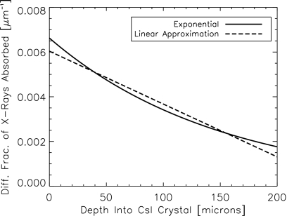
Figure 3 shows a comparison of a least-squares linear approximation with the full exponential form for an energy of 25 keV corresponding to that typically used in mammography and breast tomosynthesis. Final values for a₀ and a₁ will be determined by the 2D fit, as described in Sec. 3. For lower energies, Eq. 6 may be extended to include a z² term; however, due to the increased complexity of the solution, we maintain the linear solution for this study.

Figure 3.

Comparison of exponential x-ray absorption profile with a least-squares linear approximation for 25 keV. The exponential profile is indicated with a solid line and the linear approximation with a dashed line.

Conversion of the absorbed x rays into the emitted optical photons

We assume that, on the average, the number of optical photons produced per x ray is given by a function of x-ray energy, K(E), so that the average number of optical photons produced at a given z is written as

$$N_{\text{opt}}\left(z,\theta ,\varphi ,E\right)=K\left(E\right)N_{\text{pe}}\left(z,\theta ,\varphi ,E\right).$$ (8)

Following Gallas et al.,¹⁰K(E)=γE, where γ is a material dependent gain factor and has units of keV⁻¹. For CsI, γ≈60 photons∕keV.^{13, 14}

Self-absorption and photodetector absorption of the emitted optical photons

Some of the optical photons that are produced do not reach the photodetector because of crystal self-absorption, absorption efficiency of the photodiode layer, scatter, or other effects. We can express the number of collected optical photons that reach the base of the CsI crystal as

$$N_{\text{collect}}\left(z,\theta ,\varphi ,E\right)=N_{\text{opt}}\left(z,\theta ,\varphi ,E\right)\zeta \left(z\right),$$ (9)

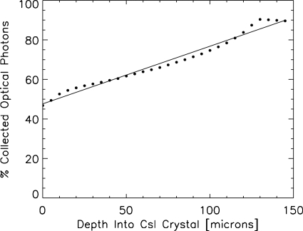
where ζ(z) is the optical collection efficiency or the percent of the emitted optical photons that are detected. The notation ζ(z) is taken from Gallas et al.¹⁰ To determine the functional form of ζ(z), we can use MANTIS as a guide. Figure 4 shows the results of simulations in MANTIS where optical photons are generated at different depths in the CsI crystal and the optical collection efficiency is recorded. MANTIS takes into account the reflectivity of the photodiode layer as well as the photodiode absorption efficiency as a function of wavelength. The MANTIS results are shown as black dots and a linear least-squares fit is shown as a solid line. Given these data we assume that the functional form of the optical collection efficiency is linear and is given by

$$\zeta \left(z\right)=b_{0}z+b_1.$$ (10)

Figure 4.

Percent of the emitted optical photons at a specific depth that reach the photodetector. Results from MANTIS simulations are shown as black dots, and a linear fit to that data is also shown. This information resulted in the use of a linear model for the crystal self-absorption.

Depth-dependent spread of optical photons

Once an optical-photon shower is produced, those photons are detected by the photodiode with a specific spread that depends on the depth at which the optical-photon shower was initiated. To determine the functional form of this spread, a series of MANTIS simulations was run in which optical-photon showers, with 10 000 optical photons each, were initiated at different depths in a 150 μm thick CsI crystal and the resulting photon spreads were recorded. The depths probed were from 0 to 145 μm at intervals of 5 μm.

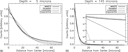
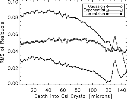
For the CsI crystal simulated in MANTIS, depths of 0–120 μm had a columnar structure, and depths of 120–150 μm corresponded to homogeneous CsI. This choice for the transition between the columnar and the homogeneous layers was motivated by the previous work where scanning electron microscope images were taken of a variety of screens to characterize the screen layers.¹⁵ Three different functional forms of the photon spread were considered: Gaussian, exponential, and Lorentzian. Each of these was fit to the normalized, radially averaged MANTIS-generated optical-photon spread at each probed depth. The normalization was performed by dividing by the maximum of the radially averaged profile. Figure 5 shows examples of these fits for two different depths (5 and 145 μm). The radially averaged MANTIS spread is shown as a solid line, while the Gaussian, Lorentzian, and exponential fits are shown as dotted, dashed, and dashed-dotted lines, respectively.

Figure 5.

Plots showing the normalized, radially averaged simulated optical-photon spread from MANTIS for two different depths; (left) 5 μm and (right) 145 μm with a zoom of the tails in the inset plot. The depth refers to the distance in the z direction between where the x-ray beam enters the CsI crystal and where the x ray is absorbed and produces the optical shower. The black lines show the radially averaged MANTIS results normalized to the maximum of the radially averaged profile. Fits of Gaussian, exponential, and Lorentzian functions are also shown. The Lorentzian shows the best overall fit to the data. In general, for optical photons produced deeper in the crystal, the Lorentzian tends to overestimate both the tails and the peak, while for shallower depths, it tends to underestimate both the tails and the peak.

The difference in width of the spreads at the two different depths is clearly demonstrated in this figure and qualitatively we can see that the Lorentzian appears to fit the MANTIS data better than either the Gaussian or exponential. In particular, the Lorentzian curve is much better than either the exponential or the Gaussian at matching the MANTIS results in the tails of the curves. The root mean squared (RMS) deviations from the MANTIS simulation results for each of these three functional forms are shown in Fig. 6. This figure verifies that the Lorentzian gives a better fit in terms of RMS deviation on the radially averaged data than either the Gaussian or exponential functional forms for every depth investigated. Therefore, we chose to model the optical-photon spread as a Lorentzian function. If we look at the fits in more detail (see Figs. 56), we can see that the Lorentzian performs somewhat better for optical photons that are absorbed deep in the crystal, but still located in the columnar zone. When the optical photons are produced closer to the crystal exit plane, the Lorentzian tends to overestimate both the tails and the peak of the spread, while for optical photons produced further from the optical detector, the Lorentzian tends to underestimate both the tails and the peak.

Figure 6.

Analysis to determine the functional form of the spread of optical photons that reach the detector after being generated at a specific depth. MANTIS simulated data were generated for depths in the crystal between 0 and 145 μm and Gaussian, exponential, and Lorentzian fits were performed to the radial average of the MANTIS results to determine the functional form of the spread. The RMS of the residuals of these fits are shown as a function of the depth at which the optical-photon shower was generated. The Lorentzian function gives the smallest RMS residuals for all depths.

The two-dimensional symmetrical version of a Lorentzian function can be written as

$$L\left(x,y\right)=\frac{c_0}{1+c_1^2\left[{\left(x-c_2\right)}^2+{\left(y-c_3\right)}^2\right]},$$ (11)

where c₀ is the amplitude of the Lorentzian, c₁ is 2∕Γ, Γ is the FWHM of the Lorentzian, c₂ is the shift of the Lorentzian in the x direction, and c₃ is the shift of the Lorentzian in the y direction. Compared to our PRF model, we find that

$$c_0=N_{\text{collect}}\left(z,\theta ,\varphi ,E\right),$$ (12)

$$c_2=z\text{\hspace{0.17em}tan\hspace{0.17em}}\theta ,$$ (13)

and

$$c_3=z\text{\hspace{0.17em}tan\hspace{0.17em}}\varphi .$$ (14)

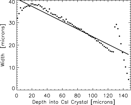
In order to determine the functional form of Γ as a function of depth, we plotted the FWHM of the Lorentzian fits as a function of depth (see Fig. 7). The reader can see that this is a complicated relationship that is poorly described by a simple analytical form. Nonetheless, in order to allow for a fully analytical solution, we approximate this relationship by a linear functional form given by

$$\Gamma =g_{0}z+g_1.$$ (15)

Figure 7.

FWHM of Lorentzian fits to MANTIS data as a function of depth where the optical photons were generated. The MANTIS data are shown as dots, while a linear fit is shown as a solid line. A linear relationship was used to model the width of the spread as a function of depth in the mathematical model.

Note that this approximation matches the MANTIS data well over the bulk of the crystal, but poorly at both very small and large depths in the crystal. Further research is needed to understand the physical origin of the downturn of Fig. 7 at small depths; however, it is likely related to the transport of photons near the interface of the organic polymer layer (a protective top coat) with the layer of columnar CsI. At very large depths, there is a sharp spike in the width because of the fact that the columnar to homogeneous CsI transition is modeled as a discontinuous change in MANTIS. Since this transition is more gradual in reality, we expect the linear approximation to apply better to experimental data. Also note that the majority of x rays are absorbed at shallow depths in the crystal because of the exponential x-ray absorption, and optical photons generated at very shallow depths in the crystal are more likely to be reabsorbed before they can reach the photodiode layer. As a result, we expect the majority of signal that makes up the PRF to arise from interactions in the middle of the crystal depth, where our linear approximation most accurately reproduces the MANTIS data.

Integrate model

The final analytical expression for the depth-dependent PRF, PRF_z, can be derived by combining Eqs. 7, 8, 9, 10, 11, 12, 13, 14, 15 to get

$${\text{PRF}}_z\left(x,y,z,\theta ,\varphi ,E\right)=\frac{\gamma E{N}_o{\mu }_{\text{pe}}\left(E\right)\left[a_0\left(E\right)z+a_1\left(E\right)\right]\left(b_{0}z+b_1\right)}{1+{\left(\frac{2}{g_{0}z+g_1}\right)}^2\left[{\left(x-z\text{\hspace{0.17em}tan\hspace{0.17em}}\theta \right)}^2+{\left(y-z\text{\hspace{0.17em}tan\hspace{0.17em}}\varphi \right)}^2\right]}.$$ (16)

In order to obtain the overall PRF, we must integrate this equation over depth,

$$\text{PRF}\left(x,y,\theta ,\varphi ,E\right)={\int }_0^{z_{\text{max}}}{\text{PRF}}_z\left(x,y,z,\theta ,\varphi ,E\right)dz.$$ (17)

The solution to this integral is given in the Appendix0. Because of the length of the solution, it is not reproduced here. Note that the contribution to the PRF from any given depth is symmetric. The asymmetry in the overall PRF comes from the depth-dependent shift of each of these contributions due to the incidence angle of the incoming x-ray beam.

CALCULATING BEST FIT COEFFICIENT VALUES AND COMPARISON WITH MANTIS

The analytical solution for the PRF (derived in the Appendix0) requires the following variables to be specified by the user: Incident angles of x-ray beam (θ,ϕ), energy of incident x-ray beam (E), and the thickness of the CsI screen (z_max). The remaining variables are p(≡γEN_oμ_pe(E)) from Eq. A3, a₀(E) and a₁(E) from Eq. 6, b₀ and b₁ from Eq. 10, and g₀ and g₁ from Eq. 15. Recall that p controls the maximum value of the overall PRF, a₀ and a₁ are the slope and intercept of the function that describes the absorption of x rays in the CsI crystal as a function of depth, b₀ and b₁ are the slope and intercept of the function that describes the optical collection efficiency, and g₀ and g₁ are the slope and intercept of the function that describes the width of the depth-dependent optical-photon spreads at the exit plane.

While approximate values for each of these variables could be taken from the analysis in Secs. 2A, 2C, 2D, the analysis in those sections was intended solely to determine an appropriate functional form for the physical process being analyzed. As a result, to determine the optimal values of these variables, we have performed a fit of the full two-dimensional PRF solution to two-dimensional MANTIS-generated PRFs. The results of Secs. 2A, 2C, 2D are used as initial guesses to this fit. The 2D fitting process allows factors that have not been explicitly included in the analytical model (i.e., columnar crystal structure, reflective substrates, and k-fluorescent x rays) to be indirectly accounted for. For example, we expect columnar structure in the CsI crystal to decrease the width of the optical spread functions as compared to a homogeneous crystal slab. By allowing the width of the spread to vary as a free parameter, this property of the crystal can be taken into account, albeit without explicit inclusion in the derivation of the analytical form of the PRF.

Two-dimensional fits of the analytical model to the MANTIS-generated PRFs were performed using a figure-of-merit (FOM) equal to the RMS normalized difference of the two PRFs within a region of interest (ROI).

A smaller FOM indicates a better fit. A mathematical definition of the FOM was given in a previous study,¹⁵ where it was used to compare MANTIS PRFs to experimental data. Here, the ROI was chosen by selecting all pixels with a signal of at least a 40th of the maximum of the MANTIS PRF. This ROI was chosen to include some of the tails of the PRFs without including regions that were noisy in the MANTIS simulations due to the number of simulated primary x rays. A sparse sampling method was used to perform the fit and was calculated as follows:

• (1)For each of the seven coefficients to be fit (p,a₀(E),a₁(E),b₀,b₁,g₀,g₁), choose five evenly spaced initial guesses. For p the initial guess was chosen as the maximum value of the MANTIS-generated PRF, while initial guesses for the other six coefficients were taken from the analysis in Secs. 2A, 2C, 2D. The range of the five initial guesses was chosen to reasonably cover the likely possible values.
• (2)Generate analytical PRFs at each angle of interest (0°, 15°, 30°, and 45° in this study) for every possible coefficient combination and calculate the corresponding FOMs for each angle. Calculate an overall FOM equal to the sum of the FOMs for each angle. Note: In this fitting scheme all seven coefficients are forced to be the same for all angles.
• (3)Identify the coefficient combination with the lowest calculated overall FOM.
• (4)Select a new set of five evenly spaced trial coefficient values, where three of those new trial coefficient values are the coefficient value with the lowest overall FOM and its two nearest neighbors. The final two trial coefficient values are directly in between the other three values. If the coefficient with the lowest overall FOM is on the edge of the grid, the grid is expanded to include a larger range of coefficient values.
• (5)Return to step (2) unless the difference between the trial coefficient values is less than 10⁻⁶ for p, 10⁻⁸ for a₀(E), and 10⁻⁵ for a₁(E), 10⁻² for b₀, 10⁻² for b₁, 10⁻⁴ for g₀, and 10⁻² for g₁. These thresholds were chosen to achieve a specific accuracy of the fitted parameter that seemed reasonable for its physical meaning. It was confirmed that the choice of these thresholds resulted in an overall FOM that stabilized during the fitting process (see text below). Once a single coefficient value has dropped below the threshold, its value is fixed at that value and the other coefficients continue to be varied.

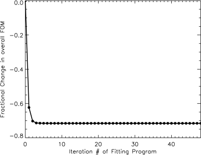
In this study, we have performed fits to a limited number of input parameters to demonstrate the ability of the analytical model to fit MANTIS-generated PRFs. Specifically, we have focused on a CsI scintillator thickness of 150 μm, an x-ray energy of 25 keV, and incidence angles of 0°, 15°, 30°, and 45°. The remainder of the CsI screen model parameters are identical to those presented in Badano et al.⁵ except for the reflective backing, where a reflectivity value of 95% was used in the current study. These input parameters are similar to system parameters found in mammography and tomosynthesis measurements. In a future study, we will perform fits over a larger range of different angles, energies, and CsI thicknesses and provide relationships to determine the optimal coefficient values for the entire range of explored input parameters. Figure 8 shows how the overall FOM changed over the course of the fitting process. Fractional change in the FOM is plotted as a function of iteration number of the 2D fitting program for the combination of 0°, 15°, 30°, and 45° incidence angles. The overall FOM decreases monotonically and reaches a stabilized value well before the end of the fitting process. The resultant coefficient values for the investigated set of parameters and choice of CsI screen are given in Table 2. Please note that these coefficients are not appropriate descriptors for a general imaging CsI screen and should not be used as representative values. The coefficients are valid only for a monoenergetic x-ray beam of 25 keV, a CsI scintillator screen with a thickness of 150 μm and similar properties to those mentioned in Badano et al.,⁵ and incidence angles ranging from 0° up to 45°. Also note that we have performed a comparison here for incidence angles in the direction of ϕ=0. We expect the analytical model to perform equally well for incidence angles in the ϕ and θ directions. The only physical effect modeled in MANTIS that changes between the θ and ϕ directions is the columnar tilt and this has been shown previously to have a small effect when integrating over large pixels (100 μm or more).¹⁵ The model should also be valid for all detector locations, assuming that the structure of the detector is independent of location.

Figure 8.

Fractional change in the overall FOM during the 2D fitting process as a function of the iteration number of the fitting program. Data are shown for a 25 keV monochromatic incoming beam, 150 μm thick CsI screen, and the combination of 0°, 15°, 30°, and 45° incidence angles. The overall FOM stabilizes well before the end of the fitting procedure.

Table 2.

Best-fit coefficient values for a 25 keV monochromatic beam, 150 μm thick CsI screen, and angles in the range of 0°–45°. These coefficients should be valid for any detector location as long as the same screen model applies. The results reported here correspond to the PRFs shown in Fig. 9.

Coefficient	Best-fit value (25 keV, 150 μm CsI)
p	0.000879
a0(E)	1.108×10−5
a1(E)	0.01429
b0	0.03
b1	37.84
g0	0.0334
g1	13.32

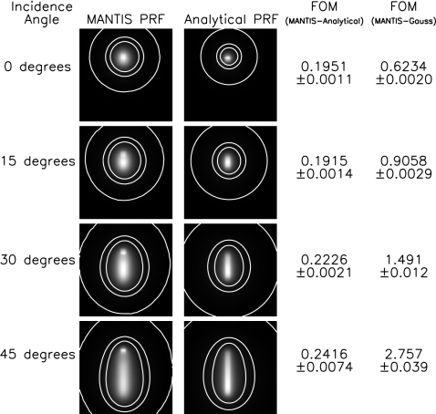
Figure 9 shows a comparison between the MANTIS-generated PRFs and the analytical model PRFs after performing the 2D fitting process. All of the PRFs shown have been generated with a CsI scintillator thickness of 150 μm, an incident x-ray energy of 25 keV, and 500 000 primary x rays. The leftmost column indicates the incidence angle of the incoming x-ray beam. The corresponding PRFs from MANTIS and the analytical model are shown in the following columns as well as the FOMs comparing those PRFs. FOM values and their errors were calculated as the mean and standard deviation of comparisons of the analytical model results with 11 independent MANTIS-generated PRFs. The rightmost column shows the FOMs from a comparison betweenMANTIS and a 2D symmetric Gaussian fit to the zero-angle MANTIS PRF. These numbers are provided to give a reference for the FOMs comparing MANTIS and the analytical model. A 2D symmetrical Gaussian fit to the zero degree data was chosen as a comparison since the use of symmetric Gaussian functions to simulate detector blur is one type of approach that is currently used in literature.² The Gaussian fit was performed using a modified version of the program gauss2dfit in the software package IDL (ITT Visual Information Solutions, Boulder, CO) that forced the widths of the 2D Gaussian in the x and y directions to be equal.

Figure 9.

Comparison of MANTIS-generated PRFs with PRFs from the analytical model after the 2D fit. All PRFs have been generated with a CsI thickness of 150 μm and an x-ray energy of 25 keV. The incident x-ray beam is modeled in MANTIS as an infinitesimal pencil beam. The incidence angle of the x-ray beam is indicated in the leftmost column, followed by the corresponding MANTIS-generated PRFs, analytical model PRFs, FOMs from the comparison between the MANTIS and analytical PRFs, and, finally, the FOM from the comparison between MANTIS and 2D symmetric Gaussian fits to the normal incidence MANTIS PRF. All PRFs are 0.315×0.315 mm² with 9 μm pixels. Contours are shown for levels of 0.01, 0.05, and 0.1 times the maximum of the PRF.

Qualitatively, from the PRF images in Fig. 9, we see that the analytical model does a good job of reproducing the MANTIS-generated PRFs at all angles investigated in this study. The analytical PRFs appear to be slightly narrower than the MANTIS PRFs and fail to reproduce a sharp peak (near the top of the PRFs) evident in the MANTIS PRFs. The tendency of the analytical model to appear slightly narrower is most likely due to the fact that the Lorentzian function underestimates the tails of the spread of the optical photons at the exit plane of the scintillator (see Sec. 2D) for the majority of x-ray absorption depths. This is the case for absorption depths from 0 to about 115 μm, where approximately 86% of 25 keV x rays that contribute to the overall PRF would be absorbed for a 150 μm thick crystal. We would expect this effect to be more dramatic for both the Gaussian and exponential models since they underestimate the tails of the optical-photon spread even more than the Lorentzian model. The analytical model fails to reproduce a bright peak evident in the MANTIS PRFs due to the linear approximation made in Sec. 2D and shown in Fig. 7. In that figure, a sharp increase in the width of the Lorentzian distribution is seen between 120 and 140 μm and clearly poorly fit by the linear approximation. As described earlier, the reason for this sharp increase in the MANTIS model is because of the discontinuous transition between the homogeneous layer and the columnar layer. Since the transition is much more gradual in reality, we do not expect this sort of behavior in experimental data (see Sec. 4 as a demonstration).

For a more quantitative comparison, we can examine the FOM values comparing the MANTIS and analytical PRFs (shown in Fig. 9). These FOM values range from 0.1951 to 0.2416 for all of the incidence angles investigated. Notably, these FOM values are relatively constant over the different incidence angles, meaning that the analytical model does a good job of reproducing the MANTIS results for all incidence angles. As a comparison, we can examine the FOMs comparing MANTIS and a 2D symmetrical Gaussian fit to the MANTIS PRF at zero degrees. This analysis gives FOMs of 0.6234±0.0020, 0.9058±0.0029, 1.491±0.012, and 2.757±0.039 for 0°, 15°, 30°, and 45°, respectively. Compared to the FOMs for the analytical model, the analytical model outperforms the Gaussian fit for all incidence angles. Interestingly, the analytical model even outperforms the 2D Gaussian fit at an incidence angle of 0°. This is likely due to the fact that a Gaussian function severely underestimates the tails of the PRF at all depths, as illustrated in Fig. 5.

COMPARISON AGAINST EXPERIMENTAL RESULTS

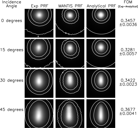
In a previous study,¹⁵ we compared the MANTIS code against experimental PRFs acquired with 40 and 70 kVp x-ray spectra (mean photon energies of 25.6 and 36.5 keV, respectively) at 0°, 15°, 30°, and 45° incidence angles for four different CsI phosphor screens. In that study, PRFs were generated in MANTIS by including details of the experimental setup in the Monte Carlo simulations. The x-ray focal spot was modeled as a 200 μm diameter circle, the pinhole and a beryllium window were modeled according to the manufacturer’s specifications, details of the CsI screen layers and columnar structure were modeled based on scanning electron microscope measurements and manufacturer’s specifications, and a fiber optic plate connecting the CsI screen to the optical detector was modeled as a solid plate of glass.

Here, we perform 2D fits of the analytical model to that same MANTIS data and then compare the resultant analytical model to the corresponding experimental data. The objective of this analysis is to evaluate the ability of the analytical model to reproduce experimental results when fit to MANTIS. We did not fit the analytical model directly to the experimental data since this will, in general, not be available. In addition, acquisition of the experimental data is achieved with a pinhole, not an infinitely small incident x-ray beam, which means it is not technically a PRF. We have completed this analysis for one of the screens (denoted as screen 2 in that paper) with a CsI thickness of 170 μm and an aluminum-coated graphite substrate (manufactured by Radiation Monitoring Devices, Inc., Watertown, MA). Only the data taken at 40 kVp (25.6 keV mean photon energy) are considered here. For the analytical model, the CsI thickness and x-ray energy values in the final analytical model solution were updated to 170 μm and 25.6 keV, respectively. Because of the small change in thickness between 150 and 170 μm, the assumption was made that the functional forms of the individual components of the analytical model were the same as for the 150 μm case. However, the reader is cautioned against using the analytical model for thicknesses other than 150 μm since further research is required to ensure that the functional forms derived in Secs. 2A, 2B, 2C, 2D hold for other thicknesses. The results of the comparison between the analytical model and the experimental data are shown in Fig. 10. Note that, as described in Freed et al.,¹⁵ the experimental data were taken with a 30 μm pinhole and a 40 kVp x-ray spectrum, so there is additional blurring as compared to the analytical model, which assumes that all the x rays are incident on the CsI crystal at the exact same position and that the incoming x-ray beam is monochromatic. The effect of the finite pinhole was partially compensated for by convolving the analytical model with a 30 μm diameter incident beam before fitting to MANTIS. The MANTIS data did take both the 30 μm pinhole and the 40 kVp x-ray spectrum into account, so this should partially mitigate the limitations of the analytical model.

Figure 10.

Comparison of the analytical model with experimental PRFs. The experimental data were taken at 40 kVp (25.6 keV mean photon energy) with a 170 μm thick CsI scintillator and a 30 μm pinhole. The analytical model was convolved with a 30 μm incident beam profile and then fit to MANTIS data that were generated by taking into account all the details of the actual CsI screen geometry. The MANTIS data were generated with a 100 μm diameter pencil beam incident on a 30 μm pinhole. The incidence angle of the incoming x-ray beam is indicated in the leftmost column, followed by the corresponding experimental PRFs, MANTIS-generated PRFs, analytical model PRFs, and FOMs from the comparison between the experimental and the analytical data. The analytical model was fit to the MANTIS results then a comparison was performed between the analytical model and the experimental data. This procedure was followed as opposed to fitting the analytical model to the experimental data since experimental PRFs will not be available for typical applications. All PRFs are 0.315×0.315 mm² with 9 μm pixels. Contours are shown for levels of 0.01, 0.05, and 0.1 times the maximum of the PRF.

The FOM values were calculated in the same way described in Sec. 3, but with an ROI that included all the points where the experimental data had a pixel signal-to-noise ratio of 50 or greater. It is important to note that because of the change in the definition of the ROI, which was necessary because of the change in the type of data involved, the FOM values in this section and Sec. 3 are not comparable. In future work, we plan to investigate alternative ways of defining the FOM such that data sets with different noise characteristics can be directly compared. Mean FOM values and their errors were calculated as the mean and standard deviation of FOM values calculated for 11 independent experimental data sets and 11 independent MANTIS-generated PRFs. The FOM values comparing the analytical PRFs with the experimental data are 0.3457±0.0036, 0.3281±0.0057, 0.3422±0.0023, and 0.3677±0.0041 for 0°, 15°, 30°, and 45°, respectively. FOMs comparing MANTIS-generated PRFs with experimental PRFs for the exact same screen investigated here were published in Ref. 15 and are 0.2944±0.0027, 0.2387±0.0039, 0.2816±0.0025, and 0.2665±0.0032 for 0°, 15°, 30°, and 45°, respectively. These FOMs are about the same magnitude as the FOMs comparing the analytical model with the experimental data. Therefore, the analytical model is able to reproduce the experimental data about as good as MANTIS is able to reproduce the experimental data. This is not surprising since the analytical model was able to reproduce MANTIS-generated PRFs well. Figure 11 shows the same data from Fig. 10, but presented in terms of the line spread function (LSF) rather than the full PRF. These LSFs were calculated by summing the PRFs along the direction perpendicular to the incoming x-ray beam and normalizing by the maximum of the summed vector. This direction is shown because it captures the anisotropy of the PRF. From these images we can see that MANTIS tends to produce a width that is too narrow at the peak and too wide at the tails. In addition, the analytical model seems to match MANTIS better than MANTIS matches the experimental data. The slight shift between the analytical model and experimental data in the plot for 45° is due to the cross-correlation algorithm used to match the data. This provides the best match between the analytical and experimental PRFs when the entire PRF is taken into account and shifts the experimental data to the right because of the asymmetric nature of the analytical PRF. In addition, the difference in width between the analytical and experimental PRFs, shown in Fig. 10, is deemphasized in the LSFs, shown in Fig. 11, because the LSF inherently mixes signal from the tails with signal from the peak. In order to improve the match between the experimental data and the analytical model, we plan to extend the analytical model to incorporate polychromatic incoming beams in future versions. Modification of the MANTIS input parameters to improve its match to experimental data may also help the analytical model to better match experimental data.

Figure 11.

Line spread functions calculated from the PRFs presented in Fig. 10 (25.6 keV, 170 μm thick CsI). The PRFs were summed along the direction perpendicular to the incoming x-ray beam and then normalized by the maximum. Experimental data, MANTIS-generated PRFs, and analytical PRFs are plotted with solid, dashed, and dotted lines, respectively. Incidence angles of 0°, 15°, 30°, and 45° are presented from left to right. MANTIS tends to underestimate the width of the peak and overestimate the width of the tails. The analytical model matches MANTIS better than MANTIS matches the experimental data. The slight shift between the analytical model and the experimental data in the plot for 45° is due to the cross-correlation algorithm used to match the data. This provides the best match between the analytical and experimental PRFs when the entire PRF is taken into account.

Finally, to demonstrate if the analytical model may be useful for describing the response of thicker screens, we performed the same analysis as above on screen 3 (450 μm and an aluminum-coated graphite substrate) from Freedet al.¹⁵ The FOMs comparing the analytical model and experimental data were 0.5847±0.0079, 0.2220±0.0190, 0.3144±0.0363, and 0.2840±0.00625 for angles of 0°, 15°, 30°, and 45°, respectively. The validation FOM values between MANTIS-generated PRFs and the same experimental data were 0.4380±0.0039, 0.2360±0.0098, 0.2592±0.0064, and 0.2421±0.0079. These initial results suggest that the analytical model described in this paper could provide reasonably accurate predictions of the response of CsI screens with thicknesses comparable to those encountered in other x-ray imaging systems, such as CT. A study is currently underway to investigate in detail the application of the model to thicker screens.

CONCLUSION

In this study, we have developed a detailed, deterministic analytical model to approximate MANTIS (Monte Carlo) generated PRFs of CsI scintillator screens for indirect x-ray detectors of 3D breast imaging systems. We have demonstrated, using quantitative FOMs, that the analytical model is able to reproduce MANTIS-generated PRFs well for a range of incidence angles and much better than a simple 2D symmetric Gaussian fit to the zero-angle MANTIS data. In addition, comparisons of the analytical model against experimental data show that the analytical model is able to reproduce experimental data about as well as MANTIS. Therefore, the analytical model produces PRFs that are comparable to those generated by MANTIS and that capture the anisotropy effects seen at large incidence angles. Most importantly, because the analytical model is a (relatively) simple mathematical expression, it can generate a PRF in only 0.1 s on a single CPU, which is less than one millionth the computational time required by MANTIS to produce a comparable (but still noisy) PRF (200 h on a single CPU). The ability of the analytical model to generate PRFs in such a short time will allow for inclusion of the detailed PRF structure that has been demonstrated with MANTIS in rigorous optimization algorithms and rapid 3D image reconstructions. This has the potential to improve lesion detection in future 3D breast imaging systems by including accurate detector blur functions in optimization of the system geometry. In addition, more detailed knowledge of the forward problem with respect to detector performance will allow for reconstructed images that are a more faithful representation of the true object.

The current work has investigated a limited set of parameters (25 keV x rays, 150 μm thick CsI, and incidence angles of 0°, 15°, 30°, and 45°) and has demonstrated generation of only four individual PRFs. In future studies, we will extend this work by performing fits of the analytical model to MANTIS-generated PRFs for a larger, but still discrete, set of parameters (x-ray energies, CsI crystal thicknesses, and incidence angles). In addition, we will develop relationships that allow for generation of the appropriate analytical model coefficient values over the entire range of investigated values so that model PRFs can be easily generated for optimization and reconstruction algorithms. The current model can also be used to derive noise transfer properties of indirect imaging detectors.

APPENDIX: INTEGRATING THE PRF EQUATION OVER DEPTH

Here we derive the solution to

$$\text{PRF}\left(x,y,\theta ,\varphi ,E\right)={\int }_0^{z_{\text{max}}}{\text{PRF}}_z\left(x,y,z,\theta ,\varphi ,E\right)dz,$$ (A1)

where

$${\text{PRF}}_z\left(x,y,z,\theta ,\varphi ,E\right)=\frac{\gamma E{N}_o{\mu }_{\text{pe}}\left(E\right)\left[a_0\left(E\right)z+a_1\left(E\right)\right]\left(b_{0}z+b_1\right)}{1+{\left(\frac{2}{g_{0}z+g_1}\right)}^2\left[{\left(x-z\text{\hspace{0.17em}tan\hspace{0.17em}}\theta \right)}^2+{\left(y-z\text{\hspace{0.17em}tan\hspace{0.17em}}\varphi \right)}^2\right]}.$$ (A2)

To simplify the notation, we can define a few variables

$$p\left(E\right)\equiv \gamma E{N}_o{\mu }_{\text{pe}}\left(E\right),$$ (A3)

$$q\equiv b_0,$$ (A4)

$$u\equiv \text{tan\hspace{0.17em}}\theta ,$$ (A5)

$$v\equiv \text{tan\hspace{0.17em}}\varphi ,$$ (A6)

$$m\equiv g_0^2+4\left(u^2+v^2\right),$$ (A7)

$$n\equiv 2g_0{g}_1-8\left(ux+vy\right),$$ (A8)

and

$$s\equiv g_1^2+4\left(x^2+y^2\right).$$ (A9)

Now our integral becomes

$${\text{PRF}}_z\left(x,y,z,\theta ,\varphi ,E\right)={\int }_0^{z_{\text{max}}}p\left(E\right)\left[a_0\left(E\right)z+a_1\left(E\right)\right]\left(qz+b_1\right)\left(\frac{g_0^2{z}^2+2g_0{g}_{1}z+g_1^2}{m{z}^2+nz+s}\right)dz.$$ (A10)

For the case of x=y=θ=ϕ=0, this integral simplifies to

$${\text{PRF}}_z\left(0,0,z,0,0,E\right)={\int }_0^{z_{\text{max}}}p\left(E\right)\left[a_0\left(E\right)z+a_1\left(E\right)\right]\left(qz+b_1\right)dz,$$ (A11)

whose solution is simply

$${\text{PRF}}_z\left(0,0,z,0,0,E\right)=p\left(E\right)\left[\left(\frac{a_{0}q}{3}\right)z_{\text{max}}^3+\left(\frac{a_0{b}_1+a_{1}q}{2}\right)z_{\text{max}}^2+a_1{b}_1{z}_{\text{max}}\right].$$ (A12)

Otherwise, we can break down the integral by multiplying it out and separating it into 12 smaller integrals (I–XII) given by

$$\text{I}\equiv p\left(E\right)a_0\left(E\right)q{g}_0^2{\int }_0^{z_{\text{max}}}\frac{z^4}{m{z}^2+nz+s}dz,$$ (A13)

$$\text{II}\equiv 2p\left(E\right)a_0\left(E\right)q{g}_0{g}_1{\int }_0^{z_{\text{max}}}\frac{z^3}{m{z}^2+nz+s}dz,$$ (A14)

$$\text{III}\equiv p\left(E\right)a_0\left(E\right)q{g}_1^2{\int }_0^{z_{\text{max}}}\frac{z^2}{m{z}^2+nz+s}dz,$$ (A15)

$$\text{IV}\equiv p\left(E\right)a_0\left(E\right)b_1{g}_0^2{\int }_0^{z_{\text{max}}}\frac{z^3}{m{z}^2+nz+s}dz,$$ (A16)

$$\text{V}\equiv 2p\left(E\right)a_0\left(E\right)b_1{g}_0{g}_1{\int }_0^{z_{\text{max}}}\frac{z^2}{m{z}^2+nz+s}dz,$$ (A17)

$$\text{VI}\equiv p\left(E\right)a_0\left(E\right)b_1{g}_1^2{\int }_0^{z_{\text{max}}}\frac{z}{m{z}^2+nz+s}dz,$$ (A18)

$$\text{VII}\equiv p\left(E\right)a_1\left(E\right)q{g}_0^2{\int }_0^{z_{\text{max}}}\frac{z^3}{m{z}^2+nz+s}dz,$$ (A19)

$$\text{VIII}\equiv 2p\left(E\right)a_1\left(E\right)q{g}_0{g}_1{\int }_0^{z_{\text{max}}}\frac{z^2}{m{z}^2+nz+s}dz,$$ (A20)

$$\text{IX}\equiv p\left(E\right)a_1\left(E\right)q{g}_1^2{\int }_0^{z_{\text{max}}}\frac{z}{m{z}^2+nz+s}dz,$$ (A21)

$$\text{X}\equiv p\left(E\right)a_1\left(E\right)b_1{g}_0^2{\int }_0^{z_{\text{max}}}\frac{z^2}{m{z}^2+nz+s}dz,$$ (A22)

$$\text{XI}\equiv 2p\left(E\right)a_1\left(E\right)b_1{g}_0{g}_1{\int }_0^{z_{\text{max}}}\frac{z}{m{z}^2+nz+s}dz,$$ (A23)

$$\text{XII}\equiv p\left(E\right)a_1\left(E\right)b_1{g}_1^2{\int }_0^{z_{\text{max}}}\frac{1}{m{z}^2+nz+s}dz.$$ (A24)

In order to solve these integrals, we make use of standard integral solutions from the CRC Standard Mathematical Tables and Formulae.¹⁶ Since integrals I–XII have some standard integrals in common, we can define the solutions to those integrals as the shown below

$$S_4\equiv {\int }_0^{z_{\text{max}}}\frac{z^4}{m{z}^2+nz+s}dz$$ (A25)

$$=[\frac{2m^2{z}_{\text{max}}^3-3nm{z}_{\text{max}}^2+6z_{\text{max}}\left(n^2-sm\right)}{6m^3}\phantom{]}$$ (A26)

$$-\left(\frac{n^3-2snm}{2m^4}\right)\left[\text{ln}\left(m{z}_{\text{max}}^2+n{z}_{\text{max}}+s\right)-\text{ln}\left(s\right)\right]$$ (A27)

$$+\left[\frac{n^4-4s{n}^{2}m+2s^2{m}^2}{m^4\sqrt{4sm-n^2}}\right]\ast \phantom{[}\left[{\text{tan}}^{-1}\left(\frac{2m{z}_{\text{max}}+n}{\sqrt{4sm-n^2}}\right)-{\text{tan}}^{-1}\left(\frac{n}{\sqrt{4sm-n^2}}\right)\right]],$$ (A28)

$$S_3\equiv {\int }_0^{z_{\text{max}}}\frac{z^3}{m{z}^2+nz+s}dz$$ (A29)

$$=[\frac{m{z}_{\text{max}}^2-2n{z}_{\text{max}}}{2m^2}\phantom{]}$$ (A30)

$$+\left(\frac{n^2-sm}{2m^3}\right)\left[\text{ln}\left(m{z}_{\text{max}}^2+n{z}_{\text{max}}+s\right)-\text{ln}\left(s\right)\right]$$ (A31)

$$+\left(\frac{3snm-n^3}{m^3\sqrt{4sm-n^2}}\right)\ast \phantom{[}\left[{\text{tan}}^{-1}\left(\frac{2m{z}_{\text{max}}+n}{\sqrt{4sm-n^2}}\right)-{\text{tan}}^{-1}\left(\frac{n}{\sqrt{4sm-n^2}}\right)\right]],$$ (A32)

$$S_2\equiv {\int }_0^{z_{\text{max}}}\frac{z^2}{m{z}^2+nz+s}dz$$ (A33)

$$=[\frac{z_{\text{max}}}{m}-\frac{n}{2m^2}\left[\text{ln}\left(m{z}_{\text{max}}^2+n{z}_{\text{max}}+s\right)+\text{ln}\left(s\right)\right]\phantom{]}$$ (A34)

$$+\frac{n^2-2sm}{m^2\sqrt{4sm-n^2}}\ast \phantom{[}\left[{\text{tan}}^{-1}\left(\frac{2m{z}_{\text{max}}+n}{\sqrt{4sm-n^2}}\right)-{\text{tan}}^{-1}\left(\frac{n}{\sqrt{4sm-n^2}}\right)\right]],$$ (A35)

$$S_1\equiv {\int }_0^{z_{\text{max}}}\frac{z}{m{z}^2+nz+s}dz$$ (A36)

$$=[\frac{1}{2m}\left[\text{ln}\left(m{z}_{\text{max}}^2+n{z}_{\text{max}}+s\right)-\text{ln}\left(s\right)\right]\phantom{]}$$ (A37)

$$-\frac{n}{m\sqrt{4sm-n^2}}\ast \phantom{[}\left[{\text{tan}}^{-1}\left(\frac{2m{z}_{\text{max}}+n}{\sqrt{4sm-n^2}}\right)-{\text{tan}}^{-1}\left(\frac{n}{\sqrt{4sm-n^2}}\right)\right]],$$ (A38)

$$S_0\equiv {\int }_0^{z_{\text{max}}}\frac{1}{m{z}^2+nz+s}dz$$ (A39)

$$=\frac{2}{\sqrt{4sm-n^2}}\left[{\text{tan}}^{-1}\left(\frac{2m{z}_{\text{max}}+n}{\sqrt{4sm-n^2}}\right)-{\text{tan}}^{-1}\left(\frac{n}{\sqrt{4sm-n^2}}\right)\right].$$ (A40)

Now the solutions to integrals I–XII are simply

$$\text{I}=p\left(E\right)a_0\left(E\right)q{g}_0^2{S}_4,$$ (A41)

$$\text{II}=2p\left(E\right)a_0\left(E\right)q{g}_0{g}_1{S}_3,$$ (A42)

$$\text{III}=p\left(E\right)a_0\left(E\right)q{g}_1^2{S}_2,$$ (A43)

$$\text{IV}=p\left(E\right)a_0\left(E\right)b_1{g}_0^2{S}_3,$$ (A44)

$$\text{V}=2p\left(E\right)a_0\left(E\right)b_1{g}_0{g}_1{S}_2,$$ (A45)

$$\text{VI}=p\left(E\right)a_0\left(E\right)b_1{g}_1^2{S}_1,$$ (A46)

$$\text{VII}=p\left(E\right)a_1\left(E\right)q{g}_0^2{S}_3,$$ (A47)

$$\text{VIII}=2p\left(E\right)a_1\left(E\right)q{g}_0{g}_1{S}_2,$$ (A48)

$$\text{IX}=p\left(E\right)a_1\left(E\right)q{g}_1^2{S}_1,$$ (A49)

$$\text{X}=p\left(E\right)a_1\left(E\right)b_1{g}_0^2{S}_2,$$ (A50)

$$\text{XI}=2p\left(E\right)a_1\left(E\right)b_1{g}_0{g}_1{S}_1,$$ (A51)

and

$$\text{XII}=p\left(E\right)a_1\left(E\right)b_1{g}_1^2{S}_0.$$ (A52)

References

- Richard S. and Siewerdsen J. H., “Cascaded systems analysis of noise reduction algorithms in dual-energy imaging,” Med. Phys. 35(2), 586–601 (2008). 10.1118/1.2826556 [DOI] [PubMed] [Google Scholar]
- Yadava G. K., Kuhls-Gilcrist A. T., Rudin S., Patel V. K., Hoffmann K. R., and Bednarek D. R., “A practical exposure-equivalent metric for instrumentation noise in x-ray imaging systems,” Phys. Med. Biol. 53(18), 5107–5121 (2008). 10.1088/0031-9155/53/18/017 [DOI] [PMC free article] [PubMed] [Google Scholar]
- Chen Y., Lo J. Y., and J. T.DobbinsIII, “Importance of point-by-point back projection correction for isocentric motion in digital breast tomosynthesis: Relevance to morphology of structures such as micro-calcifications,” Med. Phys. 34(10), 3885–3892 (2007). 10.1118/1.2776256 [DOI] [PubMed] [Google Scholar]
- Wu T., Moore R. H., Rafferty E. A., and Kopans D. B., “A comparison of reconstruction algorithms for breast tomosynthesis,” Med. Phys. 31(9), 2636–2647 (2004). 10.1118/1.1786692 [DOI] [PubMed] [Google Scholar]
- Badano A., Kyprianou I. S., Jennings R. J., and Sempau J., “Anisotropic imaging performance in breast tomosynthesis,” Med. Phys. 34(11), 4076–4091 (2007). 10.1118/1.2779943 [DOI] [PubMed] [Google Scholar]
- Badano A., Kyprianou I. S., Freed M., Jennings R. J., and Sempau J., “Effect of oblique x-ray incidence in flat-panel computed tomography of the breast,” IEEE Trans. Med. Imaging 28, 696–702 (2009). [DOI] [PubMed] [Google Scholar]
- Mainprize J. G., Bloomquist A. K., Kempston M. P., and Yaffe M. J., “Resolution at oblique incidence angles of a flat panel imager for breast tomosynthesis,” Med. Phys. 33(9), 3159–3164 (2006). 10.1118/1.2241994 [DOI] [PubMed] [Google Scholar]
- Badano A. and Sempau J., “Combined x-ray, electron, and optical Monte Carlo simulations of indirect radiation imaging systems,” Phys. Med. Biol. 51, 1545–1561 (2006). 10.1088/0031-9155/51/6/013 [DOI] [PubMed] [Google Scholar]
- Badano A., Kyprianou I. S., and Sempau J., “Anisotropic imaging performance in indirect x-ray imaging detectors,” Med. Phys. 33(8), 2698–2713 (2006). 10.1118/1.2208925 [DOI] [PubMed] [Google Scholar]
- Gallas B. D., Boswell J. S., Badano A., Gagne R. M., and Myers K. J., “An energy- and depth-dependent model for x-ray imaging,” Med. Phys. 31(11), 3132–3149 (2004). 10.1118/1.1806293 [DOI] [PubMed] [Google Scholar]
- Salvat F., Fernández-Varea J. M., and Sempau J., “PENELOPE-2006: A code system for Monte Carlo simulation of electron and photon transport,” Nuclear Energy Agency (OECD) Issy-les-Moulineaux (2006), http://www.nea.fr.
- Sempau J., Acosta E., Baró J., Fernández-Varea J. M., and Salvat F., “An algorithm for Monte Carlo simulation of coupled electron-photon transport,” Nucl. Instrum. Methods Phys. Res. B 132, 377–390 (1997). 10.1016/S0168-583X(97)00414-X [DOI] [Google Scholar]
- Knoll G., Radiation Detection and Measurement (Wiley, New York, 2000). [Google Scholar]
- Robbins D. J., “On predicting the maximum efficiency of phosphor systems excited by ionizing radiation,” J. Electrochem. Soc. 127(12), 2694–2702 (1980). 10.1149/1.2129574 [DOI] [Google Scholar]
- Freed M., Miller S., Tang K., and Badano A., “Experimental validation of Monte Carlo (MANTIS) simulated x-ray response of columnar CsI phosphor screens,” Med. Phys. 36(11), 4944–4956 (2009). 10.1118/1.3233683 [DOI] [PMC free article] [PubMed] [Google Scholar]
- CRC Standard Mathematical Tables and Formulae, 30th ed., edited by Zwillinger D. (CRC, Washington, D.C., 1996). [Google Scholar]