Calibration of Disease Simulation Model Using an Engineering Approach

Abstract

Objectives

Calibrating a disease simulation model’s outputs to existing clinical data is vital to generate confidence in the model’s predictive ability. Calibration involves two challenges: 1) defining a total goodness-of-fit score for multiple targets if simultaneous fitting is required; and 2) searching for the optimal parameter set that minimizes the total goodness-of-fit score (i.e., yields the best fit). To address these two prominent challenges, we have applied an engineering approach to calibrate a microsimulation model, the Lung Cancer Policy Model (LCPM).

Methods

First, eleven targets derived from clinical and epidemiological data were combined into a total goodness-of-fit score by a weighted-sum approach, accounting for the user-defined relative importance of the calibration targets. Second, two automated parameter search algorithms, Simulated Annealing (SA) and Genetic Algorithm (GA), were independently applied to a simultaneous search of 28 natural history parameters to minimize the total goodness-of-fit score. Algorithm performance metrics were defined for speed and model fit.

Results

Both search algorithms obtained total goodness-of-fit scores below 95 within 1,000 search iterations. Our results show that SA outperformed GA in locating a lower goodness-of-fit. After calibrating our LCPM, the predicted natural history of lung cancer was consistent with other mathematical models of lung cancer development.

Conclusion

An engineering-based calibration method was able to simultaneously fit LCPM output to multiple calibration targets, with the benefits of fast computational speed and reduced need for human input and its potential bias.

Introduction

Simulation modeling and clinical trials offer different and complementary methods of exploring the relationship between a health care intervention and health outcomes. Clinical trials compare two or more clinical interventions and are able to describe the comparative effectiveness of the different options. However, most clinical trials have a relatively short time horizon (2 - 7 years); by extrapolating from the short term trial data, modeling can estimate the longer term consequences (both positive and negative) of the intervention. In addition, clinical trials are very expensive and so rarely evaluate all the clinically relevant options; modeling can combine the results of several clinical trials, adjust for trial population differences, and estimate the incremental differences between options not compared in any one trial.

In some instances, simulation models incorporate unobservable natural history parameters to model disease development in patients. Often, estimates of logical relationships between observable parameters can be established using meta-analysis or evidence synthesis, but the values of unobservable natural history parameters must be obtained through the process of model calibration. Calibration is a process of varying the unobservable parameters until model outputs closely match existing clinical and epidemiological data.¹ After the relevant epidemiological data have been selected as calibration targets, calibrating the model to those targets consists of two parts: (1) defining how to simultaneously measure the level of discrepancy between model output and multiple calibration targets; and (2) searching for the parameter set which results in an overall minimization of that discrepancy.

Despite the importance of model calibration, there is no standard practice in the disease modeling literature for measuring the level of discrepancy between the model output and the calibration targets. Nor are there standards for how to search the parameter space such that the best parameter set is identified.

Methods of defining the level of discrepancy vary widely. Some researchers visually match the model output to the clinical data. This methodology is particularly problematic because it cannot be independently replicated: a different researcher using the same model may have selected a different parameter set.

Methods of searching the parameter space also vary widely. Some researchers manually vary input parameters in their models, while others use simple parameter search algorithms, such as grid search^{2, 3} and random search.⁴ Grid search divides each parameter value between the maximum and minimum values into regular grids. The results of all possible parameter set combinations are then compared to the calibration targets. The random search algorithm randomly picks input parameter sets within the allowable parameter space. Based on initial results, the allowable parameter region can be modified or narrowed, and searched again more thoroughly. Both methods attempt to locate the optimal parameter values by exhaustively exploring the whole parameter space. These methods will find the optimal parameter set, but are only practical for simulation models with only a few parameters.

For a disease microsimulation model with many natural history parameters, grid and random search methods cannot sample the parameter space efficiently. Using a model with 20 unobservable parameters as an example, testing only 10 values of each unknown parameter with grid or random searches will require 10²⁰ parameter sets. In practice, researchers would not test all 10²⁰ sets; typically, results from searching one area of parameter space are visually inspected and interpreted before selecting another area of parameter space to search. However, even searching a portion of those possibilities would result in a time consuming effort.

We sought to adapt calibration methodologies from the engineering literature that would enable an automated, computationally feasible, and time-efficient parameter search for comprehensive microsimulation models. Two fast parameter search algorithms commonly used in engineering simulation were identified as potentially meeting all of these criteria: Simulated Annealing (SA)^{5, 6} and Genetic Algorithm (GA).^{7, 8} Both parameter search methods were applied to the Lung Cancer Policy Model (LCPM),^{9, 10} a microsimulation model of lung cancer development, progression, detection, treatment, and survival. In this paper, we have provided examples of using these two fundamentally different optimization algorithms to perform the parameter search and compared their performance using relevant constraints and scenarios comparable to the process of initially calibrating a model, repeating the calibration of an individual component or refining the calibration.

Material and Methods

Lung Cancer Policy Model (LCPM)

The LCPM is as a comprehensive model of lung cancer, designed to evaluate screening^{10, 11} and other lung cancer control interventions. A detailed description of all components of the model is available online at the National Cancer Institute’s Cancer Intervention and Surveillance Modeling Network (CISNET) Web site (http://cisnet.cancer.gov/profiles/), but details relevant to the current study are provided here. The LCPM simulates cohorts of individuals with gender, race, and birth cohort specific smoking histories as observed for the U.S. population.^{12, 13} In each monthly cycle, an individual may develop a new cancer, or have an existing cancer grow, or develop symptoms. Lung cancers and benign pulmonary nodules can be detected through incidental imaging or scheduled screening. Cancers can also be diagnosed by an evaluation of a patient’s symptoms. Patients with suspected lung cancer receive diagnostic and staging tests, and may receive surgical or non-surgical treatment. Existing cancers may or may not be detected before an individual dies of their lung cancer or from another cause.¹ Smoking exposure is updated monthly. Model outputs include estimates of age-specific lung cancer incidence rates and distributions of lung cancer cell types and stage at diagnosis, as well as survival by stage at diagnosis.

To reflect known heterogeneity of lung cancer and allow the evaluation of a variety of interventions, the LCPM has a ‘deep’ underlying natural history model, with cell-type specific parameters for growth, invasiveness, and relationship with smoking (among others). Simulating the development and progression of 4 cell types of lung cancer with such detail required calibrating the model to estimate values of 87 unobservable natural history parameters. In this study, we applied the optimization algorithms to a subset of 28 parameters that describe the development of new lung cancers (ie, coefficients in the logistic equations for each cell type). The remaining 59 parameters related to the growth, progression, and symptom detection of existing cancers were not varied and their values were estimated in the previous calibration exercises.

Each simulated person may develop up to 3 cancers of any of 4 lung cancer cell types (adenocarcinoma with or without bronchioloalveolar carcinoma, large cell, squamous cell, and small cell), which comprise over 90% of lung cancer. The monthly probability of developing the first malignant cell is calculated using an independent logistic equation for each cancer type. Each logistic function has a type-specific intercept, type-specific coefficients for age, age², years of cigarette exposure (smoke-years, SY), an interaction term between SY and age², the average number of cigarettes smoked per day (cigarettes per day, CPD), and the years since quitting (YSQ) smoking.

Prior to beginning the calibration procedure, we eliminated implausible parameter ranges and assumed correlations between some parameters on the basis of known relationships between the incidence of lung cancer by cell type and smoking history. For example, the baseline risks dictated by the type-specific intercepts were ordered to reflect the distribution of cell types among non-smokers.^14-17 Lung cancer risk is also known to increase with age and smoking experience (SY) and lung cancer risk is known to decrease as the years since quitting (YSQ) increases.^18-21 The risk of small cell cancer is the most dramatically affected by smoking experience, and the effect of smoking cessation has the weakest effects for developing adenocarcinoma.^{16, 22} Thus, the type-specific coefficient for SY is required to have the largest magnitude for small cell cancer and the type-specific coefficient for YSQ is necessary to have the smallest magnitude for adenocarcinoma.

To account for the changes in unmeasured risk factors (in addition to the change in smoking pattern) experienced by different birth cohorts, we incorporated one gender specific birth-cohort coefficient, β_BY, into the monthly probability of lung cancer development.

Calibration Targets

With the publication of new biological and medical findings, new calibration targets are constantly incorporated into our LCPM. The version of the LCPM used in this study had 11 calibration targets (9 primary and 2 secondary targets), derived from various data sources. The primary calibration targets were cancer incidence by cell type, stage-specific survival, and stage distribution at diagnosis. Primary targets were extracted from data from the NCI’s Surveillance, Epidemiology, and End Results (SEER) Program.²³ The secondary calibration targets were age-specific mortality rates of non-smokers and lung cancer-specific mortality ratios for current (vs. never) smokers, derived from past cohort studies ²⁴ and other literature sources describing clinical experience.^{15, 17, 25, 26} All calibration targets in this study were derived from only publicly-available de-identified human subject data.

The discrepancy between the simulation model output and each calibration target was measured by the goodness-of-fit (GOF) statistic. We calculated the measure of discrepancy between each LCPM output to the corresponding calibration target (i), GOF_i, using a sum-of-squared error GOF statistic (analogous to a χ² statistic).

Method of Handling Multiple Targets

Calibrating the LCPM to multiple targets simultaneously required a definition of a global GOF statistic. We used the weighted-sum approach^{27, 28} in which weighting factors were assigned to all targets in advance of the calibration procedure to reflect the relative importance of the targets. Thus, the summary GOF_sum statistic is a linear combination of the individual statistics,

$$GO{F}_{\text{sum}}=\sum _i{W}_i\times GO{F}_i$$ (1)

where W_i is the weighting factor for the i ^th target. For the LCPM, primary calibration targets were given a weight of 1.0 and secondary calibration targets were given a weight of 0.5 to avoid overfitting to targets with possible measurement issues or dissimilar populations. Two of the secondary targets are functions of rare events (lung cancer in never smokers), so the GOF values for these two targets are large. During the initial exploratory runs prior to model calibration, the values of the weighting factors were tested to prevent them from dominating the GOF_sum during the calibration. Their units are in the inverse of the corresponding GOF_i, resulting in a unitless GOF_sum.

Calibrating to Multiple Population Cohorts

To model the US population, individual level characteristics such as age at starting smoking, cigarettes smoked per day, and age of smoking cessation, were generated by ‘smoking history generator’ provided by NCI’s Cancer Intervention and Surveillance Modeling Network (CISNET) (C.M. Anderson, personal communication). Calibration of the model for multiple populations was performed in a sequential manner, in which we initially calibrated all natural history parameters except β_BY (set at 1.0) to targets corresponding to the white male cohort born in 1930 to establish the reference values of the natural history parameters. We then estimated β_BY for the remaining cohorts by calibrating the simulation model to total lung cancer incidence corresponding to white males and females born between 1920 and 1970.

Parameter Search Algorithms

Simulated Annealing (SA)

A flow chart of the SA methodology is shown in Figure 1a. SA is analogous to the thermodynamics of freezing water or the crystallization of metal.^{5, 6} The number of defects in metal can be reduced by controlling the heating and cooling schedule during manufacturing. Heating the metal causes atoms to move from their initial positions and wander randomly (a high “free energy” state). Slowly cooling the metal to a lower free energy allows the atoms to find the most favorable configuration. The concept of SA as applied to parameter searching involves the introduction of an artificial temperature. At the initial high temperature, the search algorithm is allowed to widely explore the parameter space by accepting the parameter values with higher probabilities. By conceptualizing the model’s goodness-of-fit as a surface with peaks (poor fitting parameter sets) and valleys (better fitting parameter sets), it is apparent that bigger “jumps” avoid the algorithm falling into a local minimal goodness-of-fit. Slowly lowering the temperature allows the search to locate the parameter set with the lowest goodness-of-fit statistic. To test that the algorithm identified the unique lowest GOF statistic (the global minimum), we initiated the SA algorithm in 10 random locations in the parameter space, with each run limited to 1,000 iterations or the returned goodness-of-fit value below a predefined stopping value, GOF_stop. See section on Comparison of Search Algorithms for the definition of GOF_stop.

Figure 1.

The flow charts of Simulated Annealing and Genetic Algorithm are shown.

Genetic Algorithm (GA)

A flow chart of the GA methodology is shown in Figure 1b. The genetic algorithm is an example of evolutionary algorithms where the parameter search method is based on the principle of “survival of the fittest”.^{7, 8} The initial generation consists of a population of candidate parameter sets (analogous to chromosomes). After running the simulation model with each parameter set in the original population, the goodness-of-fit score of each individual parameter set is stored. The probability of a parameter set being selected for “reproduction” is proportional to the difference between its goodness-of-fit value and the largest goodness-of-fit value among all tested parameter sets. The parameter set with the largest goodness-of-fit value has a zero probability of reproduction and is eliminated in the reproduction process. Using a one-point crossover method,⁷ the encoded natural history parameters of two parameter sets are combined to produce a new parameter set, filling the next generation. Each newly generated parameter set is subject to random changes of individual parameters, with new values chosen within 10% of the values in either of the parent parameter sets (analogous to genetic mutation). In this study, we permitted the algorithm to repeat until either a total of 1,000 parameter sets had been tested (25 generations of 40 chromosomes) or a parameter set was identified yielding a goodness-of-fit below the same predefined stopping value (GOF_stop) in SA runs.

Comparison of Search Algorithms

We measured and compared the accuracy and speed of SA and GA parameter search algorithms for calibration of the LCPM output to the clinically observed data using a cohort of white males born in 1930. All simulation runs were performed on a LINUX High-Performance Computing (HPC) Beowulf cluster. Since the search algorithms incorporate random noise to assist the parameter exploration process, the returned results from the search algorithms are stochastic and statistical tests are required to distinguish their performances.

To compare the ability of each algorithm to find the optimal parameter set efficiently, we determined the ability of each algorithm to find the lowest GOF_sum within a specified number of iterations and the amount of time required for each algorithm to reach a specific GOF_sum target. In the accuracy comparison, each algorithm was allowed to search through the allowable parameter space for a total of 1,000 iterations; each iteration simulated a total of 500,000 hypothetical males. We performed 10 repeats using each search algorithm: 10 randomly generated starting parameter sets for SA and 10 randomly generated populations for GA. The mean minimal GOF_sum value, ${\stackrel{‒}{GOF}}_{\text{sum}}^{\min }$, from the 10 repeats was used for comparisons.

In the speed comparison, both search algorithms were allowed to search through the parameter space until they returned GOF_sum below the predefined stopping value, GOF_stop. We recorded the GOF_stop as the largest $GO{F}_{\text{sum}}^{\min }$ in the accuracy comparison. Each search algorithm was repeated 10 times in the speed comparison test. We distributed the simulation runs to the HPC Beowulf cluster using one processor per run. To simulate 500,000 individual life-histories, the LCPM would require 24 minutes processing time on a dual processor Intel® Pentium® 3.4GHz computer. Because the computational time of the simulation runs is dominated by the calculations of the life histories, SA and GA require virtually the same amount of real computational time per iteration on the same processor. The difference in CPU time between the two algorithms to complete 1000 iterations (400 hours) is less than 10 minutes. Within the cluster, there are seven types of computing nodes with different processor speeds. Hence, the real computational time per iteration depends on the hardware. Instead of reporting the real computational time, we reported the number of iterations required to reach GOF_stop.

In addition to comparing the average values, we also calculated the 95% confidence intervals using the following equation:²⁹

$$({\stackrel{‒}{T}}_1-{\stackrel{‒}{T}}_2)-z_{\alpha ∕2^{\cdot }}\sqrt{\frac{{{\sigma }^2}_1}{n_1}+\frac{{{\sigma }^2}_2}{n_2}}<{\mu }_1-{\mu }_2<({\stackrel{‒}{T}}_1-{\stackrel{‒}{T}}_2)+z_{\alpha ∕2^{\cdot }}\sqrt{\frac{{{\sigma }^2}_1}{n_1}+\frac{{{\sigma }^2}_2}{n_2}}$$ (2)

where n, T̄ and σ are the number of parameter search runs, the mean and the standard deviation of the iteration to find the stopping GOF_sum, respectively. The subscripts 1 and 2 refer to SA and GA, respectively. From the z-table for the standard normal distribution, z_α/2 =1.96. When lower and upper limits (terms on the left and right hand sides of μ₁ - μ₂) of the confidence interval are both negative, SA is faster than GA with 95% confidence. A similar equation was used for the accuracy comparison of the minimal $GO{F}_{\text{sum}}^{\min }$.

Recalibrating a Subset of Natural History Parameters

We also examined the abilities of the two parameter search algorithms to obtain optima parameter sets in a smaller parameter space, a situation often encountered when researcher are recalibrating a modified component of a simulation model. After having established th location of the optimal parameter set, we repeated the accuracy and speed comparisons whe only two natural history parameters were to be adjusted, specifically the type-specific intercept (β₀) of the logistic equations for developing adenocarcinoma and large cell lung cancer. The results are compared with the calibration results from the search with 28 parameters.

Face Validation of the Natural History Componen

The main objective of model calibration is to obtain values for the unobserved natura history parameters and the unobserved biological process which can not be experimentall determined. After model calibration, we examined two model predictions of the natural histor of lung cancer development: the lung cancer risk of current smokers, and the temporal trends of lung cancer risk for different birth cohorts.

Result

Model Calibration with Automated Search Algorithm

Examples of Parameter Searches

A typical trace of GOF_sum during a SA minimization is shown in Fig. 2. At the beginning of the SA run (high temperature), the search algorithm is allowed to explore all possible parameter values, resulting in large fluctuations in GOF_sum. At the intermediate temperature, SA avoids being trapped in the local minimum by hopping over barriers, as indicated by the arrows in Fig. 2. At low temperature, the search algorithm eventually settled on one minimum.

Figure 2.

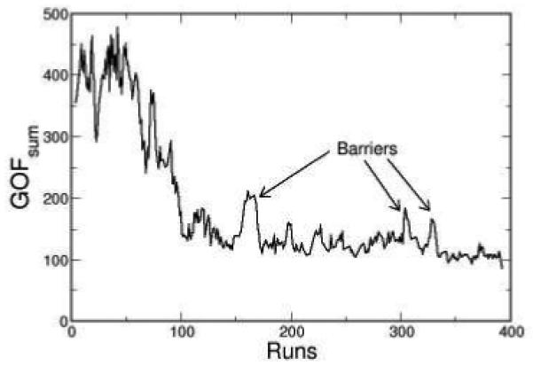
One typical trace of GOF_sum is plotted during a SA minimization. The arrows indicate three prominent barriers.

Genetic algorithm evolves the parameter search through selection and mutation. Figure 3 shows the evolution of GOF_sum as a function of generation number using GA. In the first generation, the randomly generated parameter sets yield a wide distribution of the GOF_sum values. During each reproduction cycle, the selection process forces the distribution of the GOF_sum values to converge. At the same time, the random mutations that occur in each new generation of parameter sets maintain the heterogeneity in distribution of GOF_sum as shown in Fig. 3.

Figure 3.

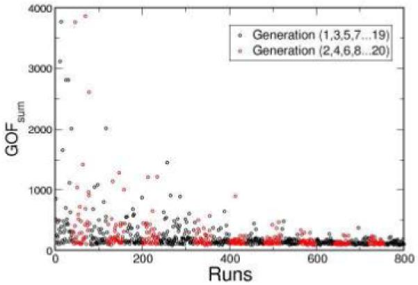
The GOF_sum scores are plotted as a function of generation number. Each circle in the graph represents the returned GOF_sum score from one chromosome. There are 40 chromosomes in each generation. In this case, GA found an acceptable minimum after 20 generations.

Comparison of Search Algorithms

We first examined the ability of both algorithms to locate the minimal GOF_sum when 28 natural history parameters are allowed to vary simultaneously. This comparison mimics the situation where researchers are performing the initial model calibration. Within 1,000 iterations, SA was able to achieve a mean minimal GOF_sum, ${\stackrel{‒}{GOF}}_{\text{sum}}^{\min }$, of 86.5 (range from 80.7 to 90.6) averaging over 10 independent parameter searches as shown in Table. 1. Within 1,000 simulation runs, GA was able to achieve ${\stackrel{‒}{GOF}}_{\text{sum}}^{\min }$ of 91.3 (85.2 to 94.1). The 95% confidence interval is: -7.56 < μ₁ - μ₂ < -2.03. The upper and lower limits of the confidence interval are both negative, indicating that SA is more efficient than GA in locating the lowest GOF_sum. The stopping GOF_sum value for the speed comparison was selected as 95 based on the rounded largest $GO{F}_{\text{sum}}^{\min }$ value obtained from GA, reflecting a typical scenario in which a parameter set must be chosen within a budgeted computational time. For the speed comparison, choosing the high stopping value also prevents the complication of some runs not achieving the stopping GOF_sum. We measured the number of iterations required to reach a GOF_sum < 95 where all 28 natural history parameters were available to be adjusted. This comparison mimics the case was where the researchers are recalibrating the model and an estimated value of ${\stackrel{‒}{GOF}}_{\text{sum}}^{\min }$ previously established. In this scenario, SA required an average of 202 iterations to reach a GOF_sum of 95. Under the same scenario, GA required an average of 294 iterations to reach a GOF_sum of 95. The values for the means and the standard deviations are shown in Table 2. The 95% confidence interval is -216.7 < μ₁ - μ₂ < 32.9. Since the two limits have opposite signs, no significant difference in speed was found between the two algorithms.

Table 1.

The comparison of the search results for fixed number of search iterations. The lower and upper limits of the 95% confidence interval around μ₁ - μ₂ are -7.56 to -2.03

	${\stackrel{‒}{GOF}}_{\text{sum}}^{\min }$	σ	n
SA	86.5	2.87	10
GA	91.3	3.41	10

Table 2.

The statistics of the results obtained from SA and GA. The indexes 1 and 2 are for SA and GA, respectively. The values of T̄ are measured and reported as the average number of iterations among 10 runs. The lower and upper limits of the 95% confidence interval is: -216.7 < μ₁ - μ₂ < 32.9

	T̄	σ	n
SA	202	113.9	10
GA	294	166.2	10

In addition to the 28 parameter searches, we have also examined the abilities of the two values are algorithms to search through only two-parameter space. In Fig. 4, the ${\stackrel{‒}{GOF}}_{\text{sum}}^{\min }$ values are plotted for both 2 and 28 parameter searches. Except the result for GA in the 28 parameter search, all of the ${\stackrel{‒}{GOF}}_{\text{sum}}^{\min }$ values are below 90. The average search times are plotted in Fig. 5. Going from 2 to 28 parameters increased the search time by 230% and 280% for SA and GA, respectively.

Figure 4.

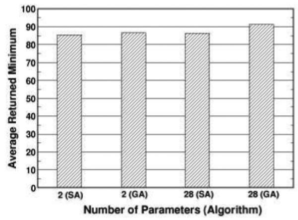
The returned minimum averaged over 10 runs for SA and GA with different number of parameters. For each search run, the algorithm is allowed to perform 1,000 iterations.

Figure 5.

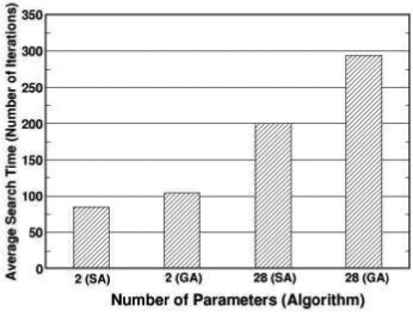
The search times averaged over 10 runs for SA and GA with different number of parameters are shown. The search time is defined as the iteration at which the search algorithm first finds a GOF_sum value below 95.

The model outputs corresponding to the parameter sets with the lowest $GO{F}_{\text{sum}}^{\min }$ for both algorithms (80.7 for SA and 85.2 for GA) are shown in Figs. 6 for selected calibration targets: overall incidence, distribution of cell type, and stage distribution of incident cancers. Both SA and GA obtained similar good fits for each of the calibration targets. Model outputs versus the remaining targets are available online (www.cisnet.cancer.gov/profiles).

Figure 6.

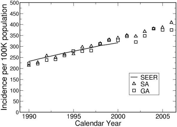
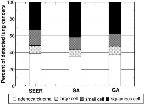
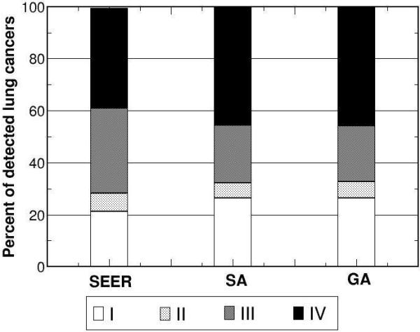
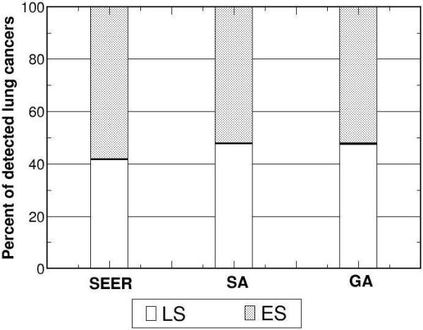
Using the returned optimal parameter set from SA and GA as inputs, the model outputs versus corresponding calibration targets for a) overall incidence, b) distribution of cell type, and stage distribution of c) non-small cell and d) small cell lung cancers for white males born in 1930 are shown.

Face Validation of Natural History Component

After model calibration, we investigated two model predictions for the natural history of lung cancer: the monthly probability of lung cancer development as a function of age and cigarettes smoked per day, and the temporal trends of lung cancer risk in the US population.

Monthly Probability of Lung Cancer Development

Since both SA and GA obtained similar good fits, we only show results using the best parameter set from SA to examine our model prediction for lung cancer development. Figure 7 shows the monthly probabilities of cancer development as a function of both age and cigarettes per day. The best natural history parameter set shows a peak in the monthly probability of developing the first malignant lung cancer cell near age 76, followed by a decrease in the monthly probability of developing lung cancer at older ages. This decreasing trend has been predicted by other published theories: increased tumor suppressor protection with age,³⁰ and the loss of proliferative ability in senescent cells.³¹

Figure 7.

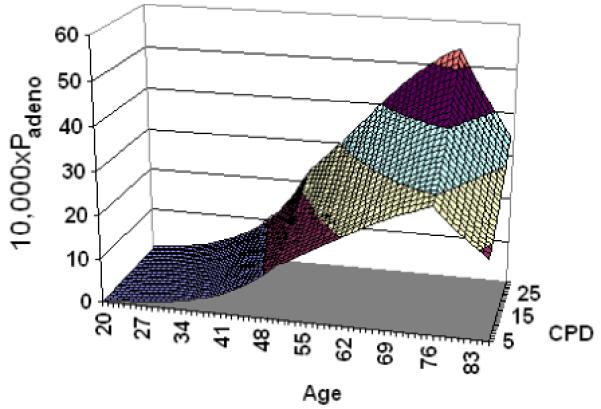
The monthly probability of cancer development for adenocarcinoma, P_adeno, is shown as a function of both age and average cigarettes smoked per day, CPD.

Population Trends in Lung Cancer

Figure 8 shows the comparison between model outputs and SEER incidence rates for white males born between 1975 and 2000. Figure 9 shows the effect of birth year on lung cancer risk, stratified by gender. For both genders, the trends level off after the 1950’s. The temporal trend for females shows a peak around 1930. Published mathematical models obtained similar results.^32-36

Figure 8.

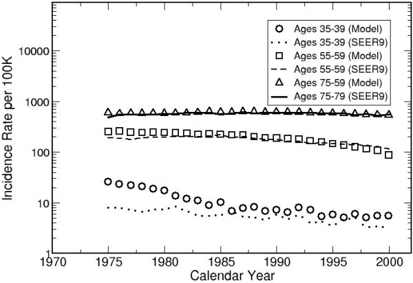
The model outputs are calibrated to the white male population in United States.

Figure 9.

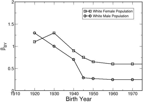
After calibrating the LCPM to the white population in the United States, β_BY is shown as a function of birth year. The results show clear gender and birth year dependencies in the monthly risk of cancer development.

Discussion

Motivated by the lack of a standard procedure to calibrate disease simulation models in the literature, we have adapted an engineering approach to calibrate the LCPM. This approach can simultaneously shorten the time spent on model calibration and minimize human-induced bias. With the ongoing release of new medical information, the LCPM is constantly being modified. This automated calibration approach is able to reduce the burden of model calibration and allow researchers to focus on model development and data analysis.

Our approach is a general procedure which can be applied to other microsimulation models. We suggest a weighted sum approach for combining multiple targets. When we varied 28 natural history parameters, our results indicate that SA is superior in locating the lowest GOF_sum. When a stopping rule is imposed by defining a specific acceptable level of GOF_sum, the average search time of SA is faster than the GA, but not significantly. For two natural history parameters, both algorithms perform equally well in model calibration. SA and GA are both faster than grid search because in grid search the computational time increases as a power function of the number of parameters as described in the introduction. This makes both SA and GA extremely attractive for calibrating disease models with a large number of parameters. In view of the fact that SA is better than or as good as GA regardless the calibration scenario. SA would be a better choice for researchers considering advanced search algorithm for automated calibration.

Our model prediction of the monthly probability of developing adenocarcinoma showed a downturn in lung cancer risk at old age. This prediction was not assumed in advance; it was purely a result of calibrating our LCPM but is in agreement with recent biological theories based on observed epidemiological data.^{30, 31} These theories still need to be verified by future clinical studies. Our approach of using logistic equations for lung cancer development is flexible enough to capture the observed epidemiological trend of lung cancer incidence at older age.

Our results indicate that the lung cancer risks (all cell types combined) of white female birth cohorts decreased from 1920 to 1945 and then leveled off. For white females, the temporal risk shows an initial increase, peaks around birth year 1930, decreases between 1930 to1950, and eventually levels off. Since population trends in smoking patterns were already incorporated by using the CISNET smoking history generator, additional effects such as increasing use of cigarette filters and improvement of the overall population health may have contributed to the decrease in the lung cancer risk for the younger birth-cohorts. Published age-cohort and age-period-cohort analyses that fitted lung cancer incidence with mathematical equations directly obtained similar results.^32-36 In Fig. 8, the LCPM over-predicted the lung cancer incidence for the youngest cohort, indicating that the lung cancer natural history of the youngest cohort is substantially different from our reference cohort of the white male born in 1930. Our method of using a single birth-cohort coefficient, β_BY, may not adequately capture the dramatically changes in population trends such as increasing use of cigarette filters and its effects on different lung cancer subtypes. In the future, we will expand β_BY to 4 cell types. The observed lung cancer incidences of different cell types will be used as calibration targets to improve our population calibration.

Manual parameter tuning, grid and random searches are inadequate to calibrate simulation models with large numbers of natural history parameters. The combination of weighted-sum method and automated parameter search algorithms offers an attractive solution for disease modelers. Our results demonstrated that this engineering approach is capable of calibrating a disease model with a large number of natural history parameters. The advantages of this novel approach are 1) estimating the natural history parameters within an acceptable time and 2) reducing human bias in the parameter search. Adapting this engineering approach also facilitates transparent communication of model calibration procedures by specifying the search algorithm.

This comparison has several limitations. First, we have not formally examined the effects of varying the ranges of allowable parameter values on the search time and accuracy of search algorithms. The best GOF_sum values are obtained within the estimated allowable parameter ranges. There are potentially lower GOF_sum values outside of the allowable parameter ranges. Second, epidemiologic studies have shown changing patterns of lung cancer incidence that are both gender and histological type-specific.^{32, 37-40} However, such effects can not be captured by the current gender specific birth-cohort coefficient, β_BY. Future expansion of the model will incorporate gender-specific birth-cohort coefficients for each histological lung cancer type.

Due to the limited time and computing resources, our approach to model calibration only explores one method of handling multiple calibration targets and two automated parameter search algorithms. In the engineering literature, there exist many excellent review articles on other techniques of optimization.^{7, 27, 41} Other disease modelers are encouraged to consider using this literature to further develop calibration procedures in disease natural history modeling.

References

- 1.McMahon PM, Zaslavsky AM, Weinstein MC, Kuntz KM, Weeks JC, Gazelle GS. Estimation of mortality rates for disease simulation models using Bayesian evidence synthesis. Medical Decision Making. 2006;26:497–511. doi: 10.1177/0272989X06291326. [DOI] [PubMed] [Google Scholar]
- 2.Goldie SJ, Weinstein MC, Kuntz KM, Freedberg KA. The costs, clinical benefits, and cost-effectiveness of screening for cervical cancer in HIV-infected women. Ann. Intern. Med. 1999;130(2):97–107. doi: 10.7326/0003-4819-130-2-199901190-00003. [DOI] [PubMed] [Google Scholar]
- 3.Mandelblatt J, Schechter CB, Lawrence W, Yi B, Cullen J. The SPECTRUM population model of the impact of screening and treatment on U.S. breast cancer trends from 1975 to 2000: principles and practice of the model methods. J Natl Cancer Inst Monogr. 2006;(36):47–55. doi: 10.1093/jncimonographs/lgj008. [DOI] [PubMed] [Google Scholar]
- 4.Fryback DG, Stout NK, Rosenberg MA, Trentham-Dietz A, Kuruchittham V, Remington PL. Chapter 7: The Wisconsin breast cancer epidemiology simulation model. JNCI Monographs. 2006;36:37–47. doi: 10.1093/jncimonographs/lgj007. [DOI] [PubMed] [Google Scholar]
- 5.Kirkpatrick S, Gelatt CD, Vecchi MP. Optimization by Simulated Annealing. Science. 1983;220:671–80. doi: 10.1126/science.220.4598.671. [DOI] [PubMed] [Google Scholar]
- 6.Wong DF, Leong HW, Liu CL. Simulated Annealing for VLSI Design. Springer; 1988. [Google Scholar]
- 7.Goldberg DE. Genetic Algorithms in Search, Optimization, and Machine Learning. Addison-Wesley Professional; Boston, MA: 1989. [Google Scholar]
- 8.Holland JH. Adaptation in Natural and Artificial Systems. Ann Arbor University of Michigan Press; 1975. [Google Scholar]
- 9.McMahon PM. Ph. D. Harvard University; Boston: 2005. Policy Assessment of Medical Imaging Utilization: Methods and Applications Health Policy. [Google Scholar]
- 10.McMahon PM, Kong CY, Johnson BE, Weinstein MC, Weeks JC, Kuntz KM, et al. Estimating Screening Effectiveness in the Mayo CT Screening Study: Results from the Lung Cancer Policy Model. Radiology. 2008;248(1):278–87. doi: 10.1148/radiol.2481071446. [DOI] [PMC free article] [PubMed] [Google Scholar]
- 11.McMahon PM, Kong CY, Weinstein M, Tramontano AC, Cipriano L, Johnson BE, et al. Adopting helical CT screening for lung cancer: Potential health consequences over a fifteen-year period. Cancer. 2008 doi: 10.1002/cncr.23962. In press. [DOI] [PMC free article] [PubMed] [Google Scholar]
- 12.U.S. Department of Health and Human Services. National Center for Health Statistics . The National Health and Nutrition Examination Survey III Data file 1988-1994. Centers for Disease Control and Prevention; Hyattsville, MD: 1997. Public Use Data file Series 11 Hyattsville, MD: Centers for Disease Control and Prevention. [Google Scholar]
- 13.National Center for Health Statistics . National Health Interview Survey. [Google Scholar]
- 14.Brownson RC, Loy TS, Ingram E, Myers JL, Alavanja MC, Sharp DJ, et al. Lung cancer in nonsmoking women. Histology and survival patterns. Cancer. 1995;75:29–33. doi: 10.1002/1097-0142(19950101)75:1<29::aid-cncr2820750107>3.0.co;2-q. [DOI] [PubMed] [Google Scholar]
- 15.Capewell S, Sankaran R, Lamb D, McIntyre M, Sudlow M. Lung cancer in lifelong non-smokers. Thorax. 1991;46:565–68. doi: 10.1136/thx.46.8.565. [DOI] [PMC free article] [PubMed] [Google Scholar]
- 16.Muscat J, Wynder E. Lung cancer pathology in smokers, ex-smokers and never smokers. Cancer Letters. 1995;88:1–5. doi: 10.1016/0304-3835(94)03608-l. [DOI] [PubMed] [Google Scholar]
- 17.Damber L, Larsson L-G. Smoking and lung cancer with special regard to type of smoking and type of cancer. A case-control study in north Sweden. British Journal of Cancer. 1986;53:673–81. doi: 10.1038/bjc.1986.111. [DOI] [PMC free article] [PubMed] [Google Scholar]
- 18.Hammond E. Smoking in relation to the death rates of one million men and women. American Cancer Society; 1966. [PubMed] [Google Scholar]
- 19.Harris JE. Trends in Smoking-Attributable Mortality, Chapter 3 Reducing the Health Consequences of Smoking, 25 Years of Progress: A Report of the Surgeon General. U.S. Department of Health and Human Services; Washington, D.C.: 1989. pp. 117–69. [Google Scholar]
- 20.Rachet B, Siemiatycki J, Abrahamowicz M, Leffondre K. A flexible modeling approach to estimating the component effects of smoking behavior on lung cancer. Journal of Clinical Epidemiology. 2004;57:1076–85. doi: 10.1016/j.jclinepi.2004.02.014. [DOI] [PubMed] [Google Scholar]
- 21.Thun MJ, Myers DG, Day-Lally C, et al. Smoking and Tobacco Control, Monograph 8: Changes in Cigarette-Related Disease Risks and Their Implication for Prevention and Control. National Cancer Institute; Washington, D.C.: 1997. Age and the exposure-response relationships between cigarette smoking and premature death in Cancer Prevention Study II. [Google Scholar]
- 22.Ebbert K, Yang P, Vachon C, Vierkant R, Cerhan J, Folsom A, et al. Lung cancer risk reduction after smoking cessation: observations from a prospective cohort of women. Journal of Clinical Oncology. 2003;21:921–26. doi: 10.1200/JCO.2003.05.085. [DOI] [PubMed] [Google Scholar]
- 23.National Cancer Institute. DCCPS. Surveillance Research Program. Cancer Statistics Branch . Database: Incidence - SEER 9 Regs Public-Use. Surveillance Research Program, National Cancer Institute SEER*Stat software; 2003. Nov 2002 Sub (1973-2000), Software. ( www.seer.cancer.gov/seerstat) version 5.3.0. Surveillance, Epidemiology, and End Results (SEER) Program. [Google Scholar]
- 24.Thun MJ, Lally CA, Flannery JT, Calle E, Flanders W, Heath CJ. Cigarette smoking and changes in the histopathology of lung cancer. J Natl Cancer Inst. 1997;89:1580–6. doi: 10.1093/jnci/89.21.1580. [DOI] [PubMed] [Google Scholar]
- 25.Beadsmoore CJ, Screaton NJ. Classification, staging and prognosis of lung cancer. European Journal of Radiology. 2003;45(1):8–17. doi: 10.1016/s0720-048x(02)00287-5. [DOI] [PubMed] [Google Scholar]
- 26.Beckles M, Spiro S, Colice G, Rudd R. Initial evaluation of the patient with lung cancer: symptoms, signs, laboratory tests, and paraneoplastic syndromes. Chest. 2003;123:97S–104S. doi: 10.1378/chest.123.1_suppl.97s. [DOI] [PubMed] [Google Scholar]
- 27.Ehrgott M. Multicriteria optimization. Springer; New York: 2000. [Google Scholar]
- 28.Freitas AA. A critical review of multi-objective optimization in data mining: a position paper. ACM SIGKDD Explorations Newsletter. 2004;6:77–86. [Google Scholar]
- 29.Kreysziq E. Advanced Engineering Mathematics ed. 9 edition Wiley; 2005. [Google Scholar]
- 30.Campisi J. Cancer and ageing: rival demons? Nature Rev. Cancer. 2003;3:339–49. doi: 10.1038/nrc1073. [DOI] [PubMed] [Google Scholar]
- 31.Pompei F, Wilson R. Age distribution of cancer: the incidence turnover at old age. Human and Ecological Risk Assessment. 2001;7:1619–50. doi: 10.1191/0748233701th091oa. [DOI] [PubMed] [Google Scholar]
- 32.Zheng T, Holford TR, Boyle P, Chen Y, Ward BA, Flannery J, et al. Time trend and the age-period-cohort effect on the incidence of histologic types of lung cancer in Connecticut, 1960-1989. Cancer. 1994;74:1556–67. doi: 10.1002/1097-0142(19940901)74:5<1556::aid-cncr2820740511>3.0.co;2-0. [DOI] [PubMed] [Google Scholar]
- 33.Holford TR. The estimation of age, period and cohort effects for vital rates. Biometrics. 1983;39:311–24. [PubMed] [Google Scholar]
- 34.Eilstein D, Uhry Z, Lim TA, Bloch J. Lung cancer mortality in France Trend analysis and projection between 1975 and 2012, using a Bayesian age-period-cohort model. Lung Cancer. 2007;59:282–90. doi: 10.1016/j.lungcan.2007.10.012. [DOI] [PubMed] [Google Scholar]
- 35.Choi Y, Kim Y, Hong YC, Park SK, Yoo KY. Temporal changes of lung cancer mortality in Korea. J Korean Med Sci. 2007;22:524–8. doi: 10.3346/jkms.2007.22.3.524. [DOI] [PMC free article] [PubMed] [Google Scholar]
- 36.Clements MS, Armstrong BK, Moolgavkar SH. Lung cancer rate predictions using generalized additive models. Biostatistics. 2005;6:576–89. doi: 10.1093/biostatistics/kxi028. [DOI] [PubMed] [Google Scholar]
- 37.Charloux A, Quoix E, Wolkove N, Small D, Pauli G, Kreisman H. The Increasing Incidence of Lung Adenocarcinoma: Reality or Artefact? A Review of the Epidemiology of Lung Adenocarcinoma. International Journal of Epidemiology. 1997;26:14–23. doi: 10.1093/ije/26.1.14. [DOI] [PubMed] [Google Scholar]
- 38.Devesa SS, Bray F, Vizcaino AP, Parkin DM. International lung cancer trends by histologic type: male:female differences diminishing and adenocarcinoma rates rising. International Journal of cancer. 2005;117:294–9. doi: 10.1002/ijc.21183. [DOI] [PubMed] [Google Scholar]
- 39.Jemal A, Chu KC, Tarone RE. Recent trends in lung cancer mortality in the United States. Journal of the National Cancer Institute. 2001;93:277–83. doi: 10.1093/jnci/93.4.277. [DOI] [PubMed] [Google Scholar]
- 40.Makitaro R, Paakko P, Huhti E, Bloigu R, Kinnula VL. An epidemiological study of lung cancer: history and histological types in a general population in northern Finland. Eur Respir J. 1999;13(2):436–40. doi: 10.1183/09031936.99.13243699. Available from http://www.ncbi.nlm.nih.gov/entrez/query.fcgi?cmd=Retrieve&db=PubMed&dopt=Citation&list_uids=10065694. [DOI] [PubMed] [Google Scholar]
- 41.Statnikov RB, Matusov JB. Multicriteria Optimization and Engineering. Chapman and Hall; New York: 1995. [Google Scholar]