Bayesian species delimitation using multilocus sequence data

Abstract

In the absence of recent admixture between species, bipartitions of individuals in gene trees that are shared across loci can potentially be used to infer the presence of two or more species. This approach to species delimitation via molecular sequence data has been constrained by the fact that genealogies for individual loci are often poorly resolved and that ancestral lineage sorting, hybridization, and other population genetic processes can lead to discordant gene trees. Here we use a Bayesian modeling approach to generate the posterior probabilities of species assignments taking account of uncertainties due to unknown gene trees and the ancestral coalescent process. For tractability, we rely on a user-specified guide tree to avoid integrating over all possible species delimitations. The statistical performance of the method is examined using simulations, and the method is illustrated by analyzing sequence data from rotifers, fence lizards, and human populations.

Accurate species delimitations are of critical importance in many areas of biology, such as conservation biology (designating endangered species), epidemiology (identifying novel pathogens), and evolutionary biology (describing patterns of diversification). Traditionally, species have been identified and described using morphological traits. However, morphological characters (e.g., coloration or feeding morphology) may often be undergoing convergent evolution as they are under similar selective pressure. Use of morphological data alone may thus underestimate the number of species and, in particular, may fail to identify cryptic species. Molecular genetic data can provide additional information about many factors related to species identification, including population identities (1), levels of recent (2, 3) or ancient (4) gene flow, degree of hybridization (5), and phylogenetic relationships among prospective species (6). Species barcoding methods assign newly sampled individuals to a set of existing species using a single-locus diagnostic sequence (7, 8). Population assignment programs use information present in multilocus genotype data to identify groups of genetically isolated individuals and infer levels of migration between groups (1–3). The groups identified by such programs are only potential species because such methods detect recent genetic isolation (over a span of even just a few generations with sufficient numbers of loci), and hundreds or thousands of generations of isolation is typical of the separation between most species. For example, major human ethnic groups are easily identified by such programs but have recently arisen (in some cases during the past 15,000 years), exchange many migrants, and do not constitute species (9). Multilocus sequence data, however, can provide support for different species delimitations using recently developed theoretical models that combine species phylogenies and gene genealogies via ancestral coalescent processes.

Conceptually, coincident splits at multiple loci in gene trees for a sample of individuals (so-called reciprocal monophyly) can provide support for the existence of genetically isolated subpopulations (and potential species) (10–12). Gene tree conflicts due to lineage sorting can be modeled using the coalescent process superimposed on a species phylogeny (13). However, most sequence data for closely related (and recently diverged) species, for which species delimitation may be most problematic, will provide poorly resolved gene trees. Gene tree conflicts may therefore also represent errors of phylogenetic inference rather than introgression or lineage sorting (14). Moreover, it is important to account for branch lengths on gene trees as well because this information is needed to distinguish between ancestral lineage sorting (via the coalescent process) and admixture among groups that form potential species. These problems can be readily overcome in a Bayesian framework by integrating over uncertainty in gene trees as well as incorporating an explicit model of lineage sorting via the coalescent process model. Here we propose a Bayesian method for calculating the posterior probabilities of potential species delimitations. A unique feature of the method is that biologists can incorporate information on plausible species membership from morphology, paleontology, and other sources by specifying different priors in the Bayesian model. For example, fossil calibrations for some well-defined species could help constrain divergence times for other potential species. This prior biological information is then combined with the genetic evidence using a Bayesian framework to generate the posterior probabilities for particular species delimitations. Clearly, to delineate species, one has to define species. Our current implementation considers “good” biological species only, in which exchange of migrants ceases as soon as species separate, and uses genomic data to examine the evidence concerning competing models of species delimitation given this species definition.

Model

The process of species delimitation can be viewed as a choice among possible equivalence sets (species) on a rooted tree structure. If we assume no admixture following the speciation event giving rise to the species, individuals that occupy the same equivalence set (species) will share three parameters: θ = 4Nμ, τ_A, and τ_D, where θ is the product of effective population size N and mutation rate μ per site; τ_A is the time at which the species arose; and τ_D is the time at which the species gave rise to a pair of descendent species (or the time at which it was sampled if an extant tip).

Let Λ be an assignment of individuals to different species, referred to as a species delimitation. Λ specifies both the number of species and the assignment of individuals to the species. Given Λ, the species are related by a phylogeny S. Thus, the species delimitation problem may be considered an extension to the phylogenetic inference problem. Consider three individuals: a, b, c. There are five possible species delimitations: {a, b, c} with one species, {a}{b, c}, {b}{c, a}, {c}{a, b}, each with two species, and {a}{b}{c} with three species. The last delimitation has three different species phylogenies. The total number of possible species trees is thus seven (Fig. S1). In general, the total number of species trees for a set of individuals is much larger than the number of possible trees conditioned on a particular species delimitation (e.g., ref. 12).

If both Λ and S are treated as unknown, a full Bayesian approach would generate the joint posterior distribution of species delimitations and species trees

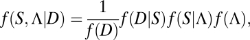where D denotes multilocus sequence data for a sample of individuals, f(D|S) is the likelihood of the data given the species phylogeny obtained by integrating over gene trees as outlined in (13), and f(S|Λ) and f(Λ) are prior distributions on species phylogenies and species delimitations, respectively. To infer only the species delimitations, for example, one could integrate the posterior probability with respect to the possible species trees (i.e., average over uncertainties in species trees). One advantage of this approach is that it can incorporate various sources of information regarding species delimitations. Namely, the prior f(Λ) may be informative and based on previously observed patterns of population substructure. If prior information is lacking, f(Λ) could be specified by assuming, for example, the Dirichlet process commonly used in Bayesian clustering (e.g., ref. 15). Similarly, f(S|Λ) can be specified either by using prior phylogenetic information from other sources or by assigning equal probabilities to rooted trees, or labeled histories, for the species. The prior on the divergence times in the species tree specifies the amount of time that genetic isolation must have persisted before we recognize genetically isolated samples as distinct species (rather than subpopulations). This is an essential component of a species definition.

Species Delimitation Using a Guide Phylogeny.

The full Bayesian approach to species delimitation outlined herein is very challenging to implement, even though all its components are computable. Here we develop a simplified Bayesian approach relying on a user-specified guide phylogeny to reduce the space of phylogenies and species delimitations that we must integrate over. The guide tree represents the phylogenetic relationships among the most subdivided possible delimitation of individuals into species that appears biologically plausible. It may be generated based on morphological characters or on geographic areas where the individuals are sampled (see below). Let S_G and Λ_G be a guide phylogeny and species delimitation, respectively. The total number of possible species delimitations, Z, depends on the specific form of the guide tree. An entirely unbalanced guide tree of s species has Z = s, but Z can be much greater. The following algorithm calculates Z for any guide phylogeny S:

• 1.Label all tips of the tree with value 1.
• 2.Move to the ancestor of each pair of labeled nodes and set the label value for the ancestral node to be x × y + 1, where x and y are the label values of the two daughter nodes, respectively.
• 3.Repeat step 2 until the root node is labeled.
• 4.Set Z to be the value of the root node label.

For example, application of this algorithm to the guide tree of Fig. 1A gives Z = 7. Let S_i and Λ_i for i ∈ (1, … , Z) be a species phylogeny and species delimitation, respectively, obtained by collapsing one or more nodes on the guide tree. We now construct a reversible-jump Markov chain Monte Carlo (rjMCMC) algorithm that successively splits or joins nodes on the guide species tree, generating the posterior probabilities for different collapsed subtrees, S_i, of the guide species tree that correspond to specific hypotheses regarding species delimitations, Λ_i. Given the guide tree, S_i is thus both a species tree and a species delimitation model. Here, we adopt the biological species concept, recognizing groups that have experienced no recent gene flow as potential species (although not requiring other evidence of reproductive isolation). Other species concepts can be accommodated in this framework, however, by modifying the priors to allow for limited hybridization, etc.

Fig. 1.

Given the guide species tree (A), each species delimitation is represented by a set of flags indicating whether each of the four ancestral nodes (6, 7, 8, 9) is collapsed (0) or resolved (1). For this guide tree, there exist seven species delimitations, shown in B, where 0000 indicates all nodes are collapsed so that there is only one species, and 1111 indicates the fully resolved tree with five species. The reversible-jump algorithm allows moves between species delimitations connected in B. The probabilities of the species delimitations under the uniform Dirichlet prior with equal probabilities for each labeled history are shown in parentheses. For example, tree 1101 has prior probability 0.2 because this tree corresponds to two labeled histories, with node 9 being older or younger than node 7, respectively (node 8 is collapsed in tree 1101). The prior with equal probabilities for the rooted trees assigns probability 1/7 for each of these species delimitations.

Posterior Probability of a Species Delimitation.

The posterior probability of species delimitation S_i is

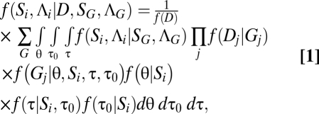where D represents sequences for L loci with D_j to be the sequences at locus j, G = {G_j}, where G_j is the gene tree at locus j, τ₀ is the time of the first divergence event (at the root) on the species phylogeny, 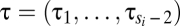is a vector of s_i – 2 nonroot node ages (in units of expected mutations per site), and s_i is the number of species in species delimitation Λ_i. Let 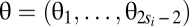be a vector of contemporary and ancestral population parameters, where θ_j = 4N_jμ, N_j is the effective population size of species j and 2s_i – 2 is the number of branches in the species delimitation tree S_i. Note that parameter θ_j is not defined if j is a contemporary species for which one or no sequences are sampled at each locus. The likelihood f(D_j|G_j) is calculated using standard methods (16) under the Jukes–Cantor mutation model (17). The prior probability density of gene trees conditional on the species tree, f(G_j|θ, S_i, τ, τ₀), is calculated using the equations in ref. 13.

Two priors were implemented for the species delimitation models (Fig. 1). The first assigns equal probabilities to rooted species trees. This is the default in the program and used in analysis of this paper. The second assigns equal probabilities to all labeled histories that are compatible with the guide species tree or its collapsed subtrees (18, 19). On a large unbalanced guide tree with many potential species, this prior assigns much greater probabilities to resolved trees than to collapsed trees, and may thus be inappropriate.

Given the species tree and root age τ₀, the rank-ordered species divergence times have the uniform Dirichlet prior

where s_i – 2 is the number of divergence times for the nonroot nodes. The root age is assigned a gamma prior τ₀ ~ G(α, β). The θ_j’s are independently and identically distributed according to another gamma distribution.

Reversible-Jump Markov Chain Monte Carlo.

The MCMC algorithm described in ref. 9 is used with the addition of a new pair of moves that either expand or collapse a node in the guide tree. The moves are between models of different dimensions, and are implemented using rjMCMC (20).

Split.

Suppose there are x previously collapsed nodes in the guide tree that may be split. A joined node is feasible for splitting if either it is the root, or its mother node is already split. Choose one of the x nodes at random for splitting. Let it be node i, and its two daughter nodes in the guide tree be j and k. The split move changes the current species-delimitation model S with parameter θ_i to a new delimitation S* with parameters θ*_i, τ*_i, θ*_j, θ*_k; other parameters are shared between the two models. Note that the new species divergence time τ_i* is constrained by the gene trees because sequences from two different species cannot coalesce until they reach their common ancestral species. The upper-bound τ_U is thus determined by scanning all gene trees to find the most recent coalescence event between two sequences of which one has ancestor j and the other has ancestor k. Our algorithm for doing this goes through all tips of the gene tree and moves toward the root, flagging each node that has j or k as ancestors. The ages of nodes that have both j and k as ancestors are used to determine τ_U. Also, τ_U should be younger than the age of the mother node on the species tree.

We tried several reversible-jump proposals, and identified two that seem to work well (algorithms 0 and 1). We describe algorithm 0 in detail and then algorithm 1 only briefly. Algorithm 0 generates three random variables, u₁, u₂, and u₃, to achieve dimension matching from parameters (θ_i, u₁, u₂, u₃) in S to (θ*_i, τ*_i, θ*_j, θ*_k) in S*, as follows:

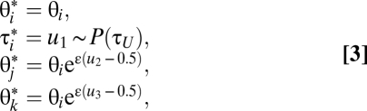where u₁ is from a parabola distribution with density f(u₁; τ_U) = 3u₁²/τ_U³ and cumulative distribution function F(u₁; τ_U) = (u₁/τ_U)³, 0 < u₁ < τ_U, and where u₂, u₃ are U(0, 1) random numbers, and ε is a fine-tuning parameter. The move makes use of the expectation that the new τ_i should be close to the upper-bound τ_U, which reflects constrains of the gene trees (Fig. S2).

The acceptance ratio for the move is

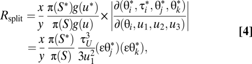where x is the number of feasible nodes for splitting in S, and y is the number of feasible nodes for joining in S*, π(S*)/π(S) is the product of the prior ratio and the likelihood ratio, and g(u) and g(u*) are the probability densities for generating random variables in the source and target. The factor (εθ_j*)(εθ_k*) is due to the two new parameters (θ_j and θ_k) in S*. However, if node j is a tip on the guide tree with at most one sequence at any locus, θ_j will not be a new parameter. The factor is replaced by (εθ_j*) or (εθ_k*) if θ_j only or θ_k only is created by the move, or by 1 if the move does not create any new θ parameter.

We use node IDs on gene trees to keep track of the population/species within which each coalescent event occurs, so that a node with ID i represents a coalescent that occurred in species i. With the creation of τ_i*, we scan the gene trees to update the node IDs: if a node has ID i but its age is younger than τ_i*, the ID is changed into j or k (for the daughter species on the guide tree).

Join.

The move for merging (joining) a pair of species proceeds as follows: identify the number, x, of possible nodes on the guide tree that may be joined; a node can be joined if its two immediate descendents are either tips or joined nodes. Choose one of them with equal probability. Let this be i and its immediate descendents be j and k. Change all node IDs j and k on gene trees into i. Parameters θ_j and θ_k, if they exist, are eliminated from the model, as is parameter τ_i. Dimension matching is achieved through

The acceptance ratio is

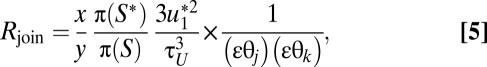where x is the number of feasible nodes for joining in S, and y is the number of feasible nodes for splitting in S*; τ_U is the upper bound for splitting node i in the target state S*. Similarly to the split move, the factor (εθ_j)(εθ_k) is used only if both θ_j and θ_k exist in species delimitation S.

Algorithm 1 proposes the new parameters θ_j and θ_k in the split move from a gamma distribution based on the current θ_i:

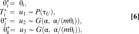where u₁ is from the parabola distribution as described (Fig. S2), and where u₂ and u₃ are gamma variables with shape α and mean mθ_i, with α and m to be fine-tuning parameters. The join move simply drops the extra parameters, as before. The acceptance ratios are

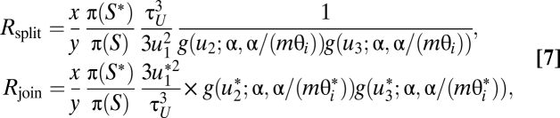where g(u;α, β) is the gamma density. Similarly, the factors g(u₂)g(u₃) and g(u₂*)g(u₃*) are used only if both parameters θ_j and θ_k exist in the split tree (in which node i is resolved).

In some cases, the algorithms did not mix well in analyzing large informative datasets. In particular, an ε too small in algorithm 0 may result in poor mixing, because the proposed values θ*_j and θ*_k in the split move may be far away from the mode of the posterior. It is advisable to use a large ε (such as 10 or 20) and to run the same analysis at least twice using both algorithms.

Species Delimitation Without rjMCMC.

For large numbers of loci and/or sequences, the rjMCMC may display mixing problems (e.g., difficulty moving between models). In such cases, a method that does not use rjMCMC may be preferable. A second method, referred to as the “τ threshold” method for species delimitation was therefore developed that does not require the use of rjMCMC. This approach involves integrating over only the most complex model (the fully resolved guide tree) using constant dimensional MCMC and using the posterior distribution of species divergence times to identify the species delimitations. The posterior probability P that the divergence time between a pair of putative species is below a threshold value (determined by the species definition) is interpreted as the probability that the two groups form a single species, whereas 1 – P is the probability that they form two distinct species. Our current implementation assigns a gamma prior on the root age τ₀, chosen such that the prior probability of recognizing either one, or two, species at the root of the species tree is 0.5. Note that this typically favors very small τ₀ values and differs from the τ₀ prior used in the rjMCMC algorithm. The rjMCMC method may be considered similar to assigning a mixture prior on τ₀ for the fully resolved guide species tree, with a point value 0 and a gamma distribution.

Results

Statistical Performance for Simulated Data.

Computer simulations were performed to examine the posterior probability associated with the correct model when the algorithm is applied to choose between the one- and two-species models. Simulations under the one-species model assumed a single-population coalescent process (21) with parameter θ = 4Nμ. Simulations under the two-species model assumed independent coalescent processes in each species, both with parameter θ, until time τ in the past when the lineages enter a common ancestral population with coalescence parameter θ. Independent gene trees were simulated at each locus, and sequences 1 kb in length were simulated on each gene tree under the Jukes–Cantor (17) mutation model.

For each of six parameter combinations, 100 replicate datasets were simulated and analyzed using our program. Two sequence sample configurations were examined: (1, 1) and (5, 5), where (i, j) indicates that i sequences are sampled from one potential species, and j sequences are sampled from the other. The divergence time parameter was either τ = θ, τ = θ/10, or τ = 0, the final case indicating a single species. The parameter θ = 0.01 was used, corresponding to an average of 1% divergence between any pair of sequences in a single population at equilibrium. To analyze data simulated with τ > 0, we assumed that the guide tree (sequence partition) was correct, whereas for data simulated with τ = 0, we assumed that the sequences in each species partition were chosen at random. This corresponds to a situation in which a biologist is sampling allopatric species versus a single panmictic species. We used a gamma (1, 10) distribution (with a mean of 0.1) for both τ and θ. In both cases, this is larger than the true values used in the simulations and allowed us to examine robustness of the posterior model probabilities when the prior is misspecified to varying degrees. Each of the 600 simulated datasets was analyzed by running two independent chains (initiated with different seeds) for 10⁶ iterations and checking for consistency of posterior model probabilities; the results were highly consistent between chains.

The results of the simulation study are summarized in Fig. 2 A and B. First we consider the sample configuration of one sequence from each population. When the true model is the one-species model (τ = 0), the posterior probability for the true (one-species model) is always greater than 90%. When the two-species model is the true model (τ = 0.01 and τ = 0.001), the posterior probability for the true model is typically low unless at least 10 loci are sampled. In these cases, the mean of the prior on τ is either one or two orders of magnitude larger than the true values. Nonetheless, with sufficient numbers of loci, and/or individuals, it is possible to identify the correct model. For a recent divergence between species (τ = 0.001), when using a prior on τ with a much larger mean, the average posterior probability of the correct model is only about 0.70, even with a sample of 100 loci (Fig. 2A). Sampling five sequences per population dramatically improves the power of the method. In that case, if the true model is a single species (τ = 0), then the posterior probability of the correct model is near 1.0 for all numbers of loci examined. If the correct model is two species with a relatively ancient divergence (τ = 0.01), the posterior probability is also near 1 for all numbers of loci examined (even for a single locus), whereas for a more recent divergence (τ = 0.001), the posterior probability still approaches 1 for as few as 10 loci (Fig. 2B). Overall, for the priors on τ and θ used in this study (which tend to specify values larger than the true simulation parameters), the method tends to be a species “lumper” if the power is low and the splits are generally conservative; if a species split has high posterior probability, it is very likely to be correct.

Fig. 2.

Mean posterior probability of the correct model across 100 replicate datasets as a function of the number of unlinked loci. The sequence at each locus was 1 kb in length. In all cases θ = 0.01. The divergence time τ = 0 corresponds to a single species, whereas τ = θ and τ = θ/10 correspond to two species with ancient and recent divergence times. In A, one sequence was sampled from each of two populations. In B, five sequences were sampled from each population.

Rotifer (Genus Rotaria).

We applied the rjMCMC method to a dataset of asexual bdelloid rotifers (22). Fontaneto et al. (22) collected Rotaria samples worldwide and conducted phylogenetic analysis using mitochondrial cytochrome oxidase I (COI) and nuclear 28S ribosomal genes. Using a species delimitation method based on estimated divergence times on gene trees (11), they suggested that the bdelloid rotifers formed independently evolving and distinct entities equivalent to species. The dataset consists of 77 mitochondrial COI sequences and 52 nuclear 28S sequences. Here, we analyze sequences from four traditionally recognized species: R. tardigrada, R. neptunoida, R. sordida, and R. macrura, with 28 COI and 17 28S sequences. The guide species tree is (((R. tardigrada, R. neptunoida), R. sordida), R. macrura), shown in Fig. 3A (ref. 22, figure 3). We assign the prior τ₀ ~ G(2, 40), with mean 0.05, and θ ~ G(2, 200), with mean 0.01 (Fig. S3). Analysis of the COI data alone generates the posterior tree probability Pr(111) = 0.997 and Pr(110) = 0.003, where 111 represents the fully resolved tree and 110 the tree with R. tardigrada and R. neptunoida collapsed into one species. On the tree 111, the posterior means of θs range from 0.06 to 0.18, whereas the posterior mean of the root age on the species tree is 0.077. Analysis of the 28S data alone led to Pr(111) = 0.750 and Pr(110) = 0.248. On the tree 111, the posterior means of θs range from 0.01 to 0.06, and the posterior mean of the root age is 0.014. The COI sequences are much more divergent and informative than the 28S sequences. To analyze both loci, we use a Dirichlet distribution to account for variable mutation rates between loci, with α = 2 (23, Eq. 4), obtaining Pr(111) = 1.000. As bdelloid rotifers are asexual, both the COI and 28S loci are haploid.

Fig. 3.

The guide species trees for the three empirical datasets analyzed in the text. (A) The guide tree for four bdelloid rotifer species/populations: Rotaria tardigrada, R. neptunoida, R. sordida, and R. macrura. (B) The guide tree for five lizard species/populations: Sceloporus tristichus (tri), S. cowlesi (cow), S. consobrinus (con), S. undulatus (und), and S. woodi (woo). (C) The guide tree for six human populations: Han Chinese (han), French Basques (bas), Melanesians (mel), Mandenka (man), Biaka (bia), and San (san).

North American Fence Lizards (Sceloporus).

We applied the rjMCMC method to a dataset for five North American fence lizards Sceloporus tristichus, S. cowlesi, S. consobrinus, S. undulates, and S. woodi (24). The sample consists of 17 individuals, with 4, 3, 4, 5, and 1 individuals for the five species, respectively. There are 29 nuclear genes in the data, with the length ranging from 254 to 1,522 sites. The number of sequences at each locus range from 10 to 17 sequences. The guide tree, shown in Fig. 3B, is based on a Bayesian species tree analysis of the mitochondrial genes (mtDNA) (24). Given the guide tree, there are seven possible trees (Fig. 1B). Until recently, four of these species (S. consobrinus, S. cowlesi, S. tristichus, and S. undulatus) were treated as a single polytypic species, with wide geographic distributions in the United States and central Mexico (25). The current species-level phylogeny, taxonomy, and phylogeographic assessment of the group is based on a mitochondrial DNA genealogy. Here we analyze the nuclear data to examine whether the mtDNA-based species are supported by nuclear genes.

We use the prior θ ~ G(2, 1000), with mean 0.002, and τ₀ ~ G(2, 1000), with mean 0.002 (Fig. S3). If all 29 loci are used, the fully resolved tree 1111 has posterior probability 1.00. The information concerning the species tree in this multiple-locus multiple-individual dataset seems overwhelming. The posterior means of the parameters under the model range from 0.002 to 0.005 for θ for the four extant species, and 0.001–0.003 for θ for the four ancestral species. The estimate of the root age τ₀ is 0.0018 with the 95% interval to be (0.0014, 0.0021). If only one locus (anonymous locus sun006) is used, the posterior probabilities are 0.54, 0.17, 0.13, 0.08, and 0.04 for trees 1111, 1101, 1110, 1001, and 1100, respectively. Even with one locus, tree 1111 reached relatively high posterior probability. This is consistent with the simulation result, which shows that the power can be high when multiple samples are taken from each species/population. The posterior for tree 1111 rises with the addition of loci, at 0.65, 0.41, 0.70, 0.97, for L = 2–5, for example.

Human Populations.

We analyzed a dataset of human ethnic populations using the τ threshold approach in which the evidence for the populations belonging to the same species is assessed through the posterior probability that τ < τ_T, a preset threshold. We set τ_T = 2 × 10⁻⁴, which means 10,000 generations of separation, based on a generation time of 20 years and a mutation rate of 10⁻⁹ mutations per site per year. The sequence data comprise samples from six populations (26), including three non-Africans: French Basques, Han Chinese, and Melanesians; and three Africans: Biaka from the Central African Republic, Mandenka from Senegal, and San from Namibia. The data consist of 20 autosomal loci, each of about 20 kb, with 18–32 sequences from each of the six populations (or 160 sequences in total) for each locus. We used the neighbor-joining tree constructed by Wall et al. (26) based on the F_ST distances between populations, shown in Fig. 3C. The same gamma prior θ ~ G(2, 1000), with mean 0.0005, is assigned to all of the 11 θ parameters. The root τ is assigned the prior τ₀ ~ G(1, 3500), with Pr(τ₀ < τ_T) = 0.50 (Fig. S3). The prior for the four other τs is specified by the Dirichlet distribution. The posterior probabilities Pr(τ_j < τ_T) are 0.98, 1.0, 1.0, 1.0, and 1.0 for nodes 7, 8, 9, 10, and 11 in the tree of Fig. 3C, respectively. Thus the analysis strongly supports the hypothesis that human individuals of all six populations are from the same species. The posterior means of the θs range from 0.0005 for the contemporary Melanesian population to 0.012 for the ancestral population of the three African populations (node 10 of Fig. 3C).

Discussion

Impact of the Guide Tree.

Here we consider a few heuristic approaches to constructing a guide tree. First, one may analyze the sequence data concatenated over loci to generate a large tree of individuals and then decide on the potential species by examining the groups defined on this tree of individuals. One may also analyze the multiple loci separately and combine the gene trees to construct a guide tree. If assignment of individuals to potential species is already accomplished, the guide tree topology may be generated using species tree methods (6, 27). Other data, such as morphological characters and geographical distributions, may also be used to construct the guide tree. Finally, the use of a few competing guide trees allows an assessment of the impact of the guide tree on the inference.

Though the use of the guide species tree has allowed us to implement the species-delimitation algorithm, it may nevertheless be a serious limitation. In our rjMCMC and τ-threshold algorithms, two individuals that are clustered into one population in the guide tree will never be separated into different species, no tree rearrangements are used to modify the guide tree, and only special cases of the guide tree (i.e., less-resolved trees generated by collapsing nodes on the guide tree) are evaluated. If the guide tree and its less-resolved special cases make up all of the species delimitations and species phylogenies that have substantial posterior probabilities, our algorithm will be a good approximation of the general algorithm outlined earlier, which considers all assignments and species trees (Λ and S). However, errors in both the assignment of individuals to populations and in the guide tree topology for the populations may cause inference errors.

For a test, the first locus in the lizard dataset was analyzed using the guide tree (((tri, con), cow), (und, woo)), which differs from the tree of Fig. 3B concerning the relationships among Sceloporus tristichus, S. consobrinus, and S. cowlesi (24). For easy comparison, we calculated the posterior probability that each node in the guide tree is collapsed, giving (((tri, con) 0.31, cow) 0.12, (und, woo) 0.20) 0.005, in comparison with (((tri, cow) 0.33, con) 0.12, (und, woo) 0.20) 0.004 for the guide tree of Fig. 3B. The two analyses thus gave very similar results, with probability 0.12 that the three concerned species should be lumped into one species, and probability 0.4–0.5% that all of the five species should be lumped into one species. The high similarity may be due to the fact that the two guide trees are quite similar.

Species Delimitation and Species Concepts.

Many natural species exchange migrants or hybridize with other species, in which case the concept of species involves some arbitrariness, and an assumption of our current model is violated. Other models of species allowing hybridization, or low levels of ongoing gene flow, could be accommodated within the same general framework. With the current model, we expect that if the method identifies distinct species, this will be more conservative if some species are allowed to undergo genetic exchange. Furthermore, our algorithm is expected to be especially useful for identifying cryptic species that are in sympatry. The impact of alternative models of speciation allowing migration etc. on the statistical performance of our method and the similarities and differences between our algorithm and population assignment algorithms, such as structure (1), merit further study. At a minimum, species delimitation should rely on many kinds of data, such as morphological, behavioral, and geographical evidence. Studies of behavior, estimation of the frequency and fitness of hybrids, and so on are essential in defining species, although coalescent analysis of genomic data provides valuable information.

Convergence and Mixing.

For most empirical datasets analyzed herein, convergence and mixing problems did not arise. In most cases, 50,000 iterations were sufficient to achieve convergence; multiple independent chains were run and yielded highly consistent estimates of posterior probabilities. The human dataset, which involved a large number of sequences and loci, did not mix well under the rjMCMC model, but consistent estimates could be obtained using the second parameter-based model of species inference. Careful adjustment of mixing parameters and monitoring of the results from independent chains for consistency is advised, especially when many loci or sequences are analyzed.

The algorithms developed in this paper are implemented in the C program bpp, which replaces MCMCcoal (13). The computation is proportional to the number of loci, and is affected more by the number of sequences in the alignments than by the number of potential species on the guide tree. On current personal computers, it seems feasible to analyze medium-sized datasets with ~10 species and ~100 sequences for a finite number of loci.

References

- 1.Pritchard J, Stephens M, Donnelly P. Inference of population structure using multilocus genotype data. Genetics. 2000;155:945–959. doi: 10.1093/genetics/155.2.945. [DOI] [PMC free article] [PubMed] [Google Scholar]
- 2.Rannala B, Mountain J. Detecting immigration by using multilocus genotypes. Proc Natl Acad Sci USA. 1997;94:9197–9201. doi: 10.1073/pnas.94.17.9197. [DOI] [PMC free article] [PubMed] [Google Scholar]
- 3.Wilson G, Rannala B. Bayesian inference of recent migration rates using multilocus genotypes. Genetics. 2003;163:1177–1191. doi: 10.1093/genetics/163.3.1177. [DOI] [PMC free article] [PubMed] [Google Scholar]
- 4.Beerli P, Felsenstein J. Maximum likelihood estimation of a migration matrix and effective population sizes in subpopulations by using a coalescent approach. Proc Natl Acad Sci USA. 2001;98:4563–4568. doi: 10.1073/pnas.081068098. [DOI] [PMC free article] [PubMed] [Google Scholar]
- 5.Anderson E, Thompson E. A model-based method for identifying species hybrids using multilocus genetic data. Genetics. 2002;160:1217–1229. doi: 10.1093/genetics/160.3.1217. [DOI] [PMC free article] [PubMed] [Google Scholar]
- 6.Liu L, Yu L, Kubatko L, Pearl DK, Edwards SV. Coalescent methods for estimating phylogenetic trees. Mol Phylogenet Evol. 2009;53:320–328. doi: 10.1016/j.ympev.2009.05.033. [DOI] [PubMed] [Google Scholar]
- 7.Matz MV, Nielsen R. A likelihood ratio test for species membership based on DNA sequence data. Philos Trans R Soc Lond B Biol Sci. 2005;360:1969–1974. doi: 10.1098/rstb.2005.1728. [DOI] [PMC free article] [PubMed] [Google Scholar]
- 8.Abdo Z, Golding GB. A step toward barcoding life: A model-based, decision-theoretic method to assign genes to preexisting species groups. Syst Biol. 2007;56:44–56. doi: 10.1080/10635150601167005. [DOI] [PubMed] [Google Scholar]
- 9.Rosenberg N, et al. Genetic structure of human populations. Science. 2002;298:2381–2385. doi: 10.1126/science.1078311. [DOI] [PubMed] [Google Scholar]
- 10.Knowles LL, Carstens BC. Delimiting species without monophyletic gene trees. Syst Biol. 2007;56:887–895. doi: 10.1080/10635150701701091. [DOI] [PubMed] [Google Scholar]
- 11.Pons J, et al. Sequence-based species delimitation for the DNA taxonomy of undescribed insects. Syst Biol. 2006;55:595–609. doi: 10.1080/10635150600852011. [DOI] [PubMed] [Google Scholar]
- 12.O'Meara BC. New heuristic methods for joint species delimitation and species tree inference. Syst Biol. 2010;59:59–73. doi: 10.1093/sysbio/syp077. [DOI] [PMC free article] [PubMed] [Google Scholar]
- 13.Rannala B, Yang Z. Bayes estimation of species divergence times and ancestral population sizes using DNA sequences from multiple loci. Genetics. 2003;164:1645–1656. doi: 10.1093/genetics/164.4.1645. [DOI] [PMC free article] [PubMed] [Google Scholar]
- 14.Yang Z. Likelihood and Bayes estimation of ancestral population sizes in hominoids using data from multiple loci. Genetics. 2002;162:1811–1823. doi: 10.1093/genetics/162.4.1811. [DOI] [PMC free article] [PubMed] [Google Scholar]
- 15.Huelsenbeck JP, Andolfatto P. Inference of population structure under a Dirichlet process model. Genetics. 2007;175:1787–1802. doi: 10.1534/genetics.106.061317. [DOI] [PMC free article] [PubMed] [Google Scholar]
- 16.Felsenstein J. Evolutionary trees from DNA sequences: A maximum-likelihood approach. J Mol Evol. 1981;17:368–376. doi: 10.1007/BF01734359. [DOI] [PubMed] [Google Scholar]
- 17.Jukes TH, Cantor CR. Mammalian Protein Metabolism. Vol. 3. New York: Academic; 1969. Evolution of protein molecules; pp. 21–132. [Google Scholar]
- 18.Edwards A. Estimation of the branch points of a branching diffusion process. J R Stat Soc B. 1970;32:155–174. [Google Scholar]
- 19.Rannala B, Yang Z. Probability distribution of molecular evolutionary trees: A new method of phylogenetic inference. J Mol Evol. 1996;43:304–311. doi: 10.1007/BF02338839. [DOI] [PubMed] [Google Scholar]
- 20.Green P. Reversible jump Markov chain Monte Carlo computation and Bayesian model determination. Biometrika. 1995;82:711–732. [Google Scholar]
- 21.Kingman J. On the genealogy of large populations. J Appl Probab. 1982;19:27–43. [Google Scholar]
- 22.Fontaneto D, et al. Independently evolving species in asexual bdelloid rotifers. PLoS Biol. 2007;5:914–921. doi: 10.1371/journal.pbio.0050087. [DOI] [PMC free article] [PubMed] [Google Scholar]
- 23.Burgess R, Yang Z. Estimation of hominoid ancestral population sizes under Bayesian coalescent models incorporating mutation rate variation and sequencing errors. Mol Biol Evol. 2008;25:1979–1994. doi: 10.1093/molbev/msn148. [DOI] [PubMed] [Google Scholar]
- 24.Leache AD. Species tree discordance traces to phylogeographic clade boundaries in North American fence lizards (Sceloporus) Syst Biol. 2009 doi: 10.1093/sysbio/syp057. in press. [DOI] [PubMed] [Google Scholar]
- 25.Leache A, Reeder T. Molecular systematics of the Eastern fence lizard (Sceloporus undulatus): A comparison of parsimony, likelihood, and Bayesian approaches. Syst Biol. 2002;51:44–68. doi: 10.1080/106351502753475871. [DOI] [PubMed] [Google Scholar]
- 26.Wall JD, et al. A novel DNA sequence database for analyzing human demographic history. Genome Res. 2008;18:1354–1361. doi: 10.1101/gr.075630.107. [DOI] [PMC free article] [PubMed] [Google Scholar]
- 27.Heled J, Drummond AJ. Bayesian inference of species trees from multilocus data. Mol Biol Evol. 2010;27:570–580. doi: 10.1093/molbev/msp274. [DOI] [PMC free article] [PubMed] [Google Scholar]
Associated Data
This section collects any data citations, data availability statements, or supplementary materials included in this article.