Responses of terrestrial ecosystems and carbon budgets to current and future environmental variability

Abstract

We assess the significance of high-frequency variability of environmental parameters (sunlight, precipitation, temperature) for the structure and function of terrestrial ecosystems under current and future climate. We examine the influence of hourly, daily, and monthly variance using the Ecosystem Demography model version 2 in conjunction with the long-term record of carbon fluxes measured at Harvard Forest. We find that fluctuations of sunlight and precipitation are strongly and nonlinearly coupled to ecosystem function, with effects that accumulate through annual and decadal timescales. Increasing variability in sunlight and precipitation leads to lower rates of carbon sequestration and favors broad-leaved deciduous trees over conifers. Temperature variability has only minor impacts by comparison. We also find that projected changes in sunlight and precipitation variability have important implications for carbon storage and ecosystem structure and composition. Based on Intergovernmental Panel on Climate Change model estimates for changes in high-frequency meteorological variability over the next 100 years, we expect that terrestrial ecosystems will be affected by changes in variability almost as much as by changes in mean climate. We conclude that terrestrial ecosystems are highly sensitive to high-frequency meteorological variability, and that accurate knowledge of the statistics of this variability is essential for realistic predictions of ecosystem structure and functioning.

Changes in climate expected in the next century (1) are likely to have important consequences for the structure, composition, and functioning of terrestrial ecosystems (2–4). Mean climate (5, 6) and climate variability are projected to shift in concert (7); for example, warmer climate may be associated with greater variability in the northeastern United States (8), increasing variability of rainfall intensity during the South Asian monsoon (9), and increasing frequency of heat waves (10).

Changes in the intermittent temporal distribution of meteorological variables are recognized to have nonlinear effects on hydrological processes such as evaporation and infiltration (11), requiring that high-frequency variability of meteorological drivers be accurately represented in hydrological models (12). It is understood that ecosystems also respond nonlinearly to environmental variation (13), but there has been little investigation into the effects of high-frequency variability on the terrestrial biosphere. Some studies of climate change effects on terrestrial ecosystems have used monthly averaged climatology, eliminating intermittent variability altogether (14–16); others use meteorological products derived from reanalysis (17, 18) or general circulation models (19, 20). The high-frequency variations of these products result from parameterized (unresolved) processes, and are generally not subjected to close scrutiny. But ecosystems respond nonlinearly to a wide range of environmental variations. Photosynthesis is a nonlinear function of solar radiation and temperature (21). Soil respiration often spikes after episodic precipitation events (22). Plant growth and mortality respond strongly to extreme events (e.g., droughts, hurricanes), and also to synoptic-scale fluctuations (23).

In this paper, we assess the influence of meteorological variability on ecosystem function and development for typical forest ecosystems in the northeastern United States, using the Ecosystem Demography model version 2 (ED2) biosphere model (24, 25) and nearly 10 years of eddy-flux measurements. We assess how strongly this system responds to high-frequency variability of sunlight, temperature, and precipitation, and identify the most important statistical measures and the underlying mechanisms for response. ED2 realistically simulates the physiological functioning, growth, death, and recruitment of individual plants and of the whole forest ecosystem, including regional structure and vegetation dynamics, for timescales from hours to decades (Materials and Methods) (24, 25). We find large, systematic differences in ecosystem functioning and the resulting structure and composition of the forest when ED2 is driven by observed hourly meteorological forcing as compared with meteorological drivers that have the same mean values but fail to reproduce high-frequency temporal variation, including sophisticated products generally considered suitable for ecosystem-climate studies.

Results

ED2 was initialized using observed stand composition and carbon stocks at Harvard Forest, and driven with 10 years of hourly meteorological data from the site (S_full), monthly averaged hourly mean values of the same data (S_mm; Fig. 1), and other datasets (see below). Removal of the high-frequency variability enhanced decadal net ecosystem productivity (NEP) by 50%, from 4.6 tons of carbon per hectare per year (tC ha⁻¹ y⁻¹) to 3.1 tC ha⁻¹ y⁻¹. Both gross primary productivity (GPP) and total ecosystem respiration (R_tot) were artificially elevated (Fig. 1), but the effect was much larger for GPP (16%; 15.4 tC ha⁻¹ y⁻¹ versus 13.3 tC ha⁻¹ y⁻¹) than for R_tot (6%). A similar nonlinear response was found for the whole northeastern region in a 100-yr integration (Fig. 2A): Mean NEP was artificially enhanced by more than 50% (1.0 tC ha⁻¹ y⁻¹ versus 0.63 tC ha⁻¹ y⁻¹) (SI Text and Fig. S1).

Fig. 1.

Simulated carbon fluxes at Harvard Forest (42.5°N, 72.1°W). Net ecosystem productivity (NEP; red curves), gross primary productivity (GPP; green curves), and ecosystem respiration (R_tot; blue curves) were all lower in S_full versus S_mm.

Fig. 2.

Impacts of meteorological variability on ecosystem structure. (A) Regional above-ground biomass (AGB) differences between S_full and S_mm after a 100-year integration. (B) Time series of AGB (black curves), hardwood AGB (red curves), and conifer AGB (blue curves) averaged over the region (A). (C and D) Above-ground biomass at the end of the 100-year simulation at a site in Maine (46.25°N, 69.25°W), partitioned by plant functional type and tree diameter at breast height (DBH). (C) The predicted forest composition in the presence of meteorological variability. (D) The corresponding distribution for the monthly mean simulation.

Altered meteorological variability had long-term consequences for simulated ecosystem structure and composition. With 100 years of monthly averaged meteorological forcing, above-ground biomass (AGB) in the region increased by 20%. The largest increases were in northern areas (Fig. 2A), reflecting stronger enhancements for conifers (Fig. 2B): AGB more than doubled for conifers, but was only 13% higher for hardwoods, in S_mm versus S_full (Fig. 2B). Stand composition shifted in favor of conifers, especially in the mixed coniferous-hardwood forests typical of the central and southern parts of the region (Fig. 2 C and D and Fig. S2).

The model's differential response of conifers versus hardwoods to meteorological variability reflects the importance of conifer photosynthesis during springtime, when meteorological variance is especially large and thus the nonlinear response to variability has a larger effect. Because hardwoods are transitioning to/from dormancy, they are affected far less by meteorological variability during this period.

It is not surprising that the full hourly variance for sunlight reduces simulated GPP and growth rates (26), because light-use efficiency (indicated by the slope of the relationship between GPP and irradiance level) is highest at low irradiance levels and declines markedly at high irradiance (Fig. S3). However, there are differences in the shapes of the GPP-sunlight curves (Fig. S3, undotted lines), showing that much of the difference between S_full and S_mm results from two unexpected factors (i): an indirect effect of precipitation variability arising from canopy interception, and (ii) the compounding effect of changing forest composition over time. In simulations with static forest composition and interception disabled (S_full-ic and S_mm-ic; dotted lines in Fig. S3), the GPP-light curves are nearly identical. (Because this reduced model does not preserve ecosystem water balance, soil moisture, GPP, and NEP are not the same.)

ED2 utilizes the widely accepted Farquhar/Ball-Berry/Collatz photosynthesis formulation, which predicts that GPP declines at high temperature and low humidity, as occurs during the summer daytime growing season conditions in this forest (specifically, sunlit, temperature > 14 °C, intercellular CO₂ ∼250 parts per million). Intercepted precipitation increases GPP by cooling leaves and elevating canopy humidity (cf ref. 27). Analysis of eddy-flux data from Harvard Forest confirms that this effect actually occurs: For a given solar input, a wet canopy does indeed have a higher photosynthetic rate than a dry canopy (Fig. 3). Reduced-variability (S_mm) simulations yield unrealistic, near-continuous wetting of the canopy, artificially elevating GPP (Table 1; Fig. 4). Meteorological variability primarily affects GPP; changes in simulated respiration (both by plants and soils) are secondary responses to changes in GPP (SI Text).

Fig. 3.

Observed hourly net carbon uptake as a function of incoming solar radiation in July. Days with >1 mm of rain (solid curve) have larger carbon uptake than drier days at the same light levels, especially at the highest irradiances.

Table 1.

Precipitation and radiation variability for different meteorological drivers and the consequences for GPP

	σprecip (mm h−1)	σsolar (W m−2)	Simulated GPP (tC ha−1 y−1)	Fitted GPP (tC ha−1 y−1)
Sfull	333	225	13.1	13.7
Smm	059	197	15.4	15.5
ECMWF	405	214	14.5	14.0
NCEP	455	204	14.5	14.3
GFDL	372	242	12.2	12.8
CNRM	311	229	13.5	13.6
GISS	348	253	11.6	12.3
ISCCP	333	213	14.0	14.2

The simulated GPP was derived from an 8-year ED2 simulation and the fitted GPP was derived from Eq. 1. σ, SD.

Fig. 4.

Dependence of gross primary productivity (GPP) and precipitation and radiation variability. The X-Y locations of the points indicate the different levels of precipitation and radiation variability present in different meteorological forcing datasets (Table 1). The Z locations of the points indicate the GPP that is simulated when the ED2 biosphere model is forced with each meteorological dataset. The dependence of GPP on meteorological variability is largely captured by Eq. 1, which is depicted in the figure as the planar surface. Note that the surface has an accompanying thickness, ranging from 0.56 to 0.65 tC ha⁻¹ y⁻¹, arising from the uncertainty in the estimated parameters in Eq. 1 (intercept: 24.5 ± 0.4; coefficient of σ_precip: −2.2 ± 0.2; coefficient of σ_solar: −0.045 ± 0.002). However, this has been omitted for simplicity.

To confirm our diagnosis of the mechanism, we used the monthly means, variances, and covariances of sunlight, temperature, and precipitation from observed weather over 8 years at Harvard Forest (SI Text) to parameterize a climate generator, which allowed us to arbitrarily adjust the variances and covariances of the meteorological drivers while keeping their means unchanged. We then used the climate generator to conduct thousands of ecosystem simulations, adjusting variances and covariances of the different meteorological drivers over broad ranges that encompassed the range of meteorology variability found in the various forcing datasets. This analysis showed that the key higher-order components of temporal variability were the SDs of precipitation (σ_precip) and sunlight (σ_solar), and that simulated annual GPP was accurately predicted by a simple bivariate linear equation:

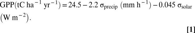Accurate representation of precipitation and radiation variances in the climate generator resulted in accurate simulation of annual carbon fluxes and associated dynamics of above-ground biomass and forest composition (SI Text). Within-month variance in temperature and covariances among the environmental parameters were not statistically significant predictors of annual GPP. We also derived a monthly analog for Eq. 1 (SI Text; Tables S1 and S2).

We found that the effects of meteorological variability shown here for monthly mean forcing (S_mm) apply directly to sophisticated meteorological drivers, including European Centre for Medium-Range Weather Forecasts (ECMWF) ERA-40 and National Centers for Environmental Prediction (NCEP) reanalysis data (28, 29), the Geophysical Fluid Dynamics Laboratory (GFDL), Goddard Institute for Space Studies (GISS), and Centre National de Recherches Météorologiques (CNRM) atmosphere-ocean general circulation models (AOGCMs) (30–32), and International Satellite Cloud Climatology Project (ISCCP) radiation (33) (Fig. 4; Table 1). To isolate the effects of variability, means of all meteorological drivers were adjusted to match the observations. In simulations using reanalysis and ISCCP data, GPP values were elevated because σ_solar was smaller than observed, likely due to grid size and/or parameterizations of boundary-layer processes. One AOGCM, CNRM, produced sunlight and precipitation variability and resulting GPP remarkably close to S_full, whereas the GFDL and GISS AOGCMs had excessively high levels of radiation and precipitation variability, resulting in significantly reduced GPP (Fig. 4). These differences led to large discrepancies in the magnitude of the terrestrial carbon sink: 10% in GPP, 25% in NEP, and 60% in AGB (Fig. S4) over 8 years. The variations would potentially be greater over longer periods as ecosystem structure evolves.

We explored how future changes in climate variability might affect carbon fluxes by comparing 8-year simulations at Harvard Forest forced with GFDL and CNRM SRESA2 meteorological outputs for the 2090s against similar simulations using meteorological output from 20th-century simulations. All means were adjusted to be equal to the 1990s observations (raw means are given in Table S3). In the GFDL forcing dataset, variability of precipitation increased in the 2090s, but solar radiation variability decreased (Table 2), partially offsetting each other and leading to a small increase in GPP (0.28 tC ha⁻¹ y⁻¹; Table 2), about 12% of the difference between S_mm and S_full. The increase in ecosystem respiration was only about half as large as the increase in GPP, indicating an increase in carbon storage in the ecosystem due solely to changes in high-frequency variances. Indeed, we found that above-ground biomass increased at a rate 0.08 tC ha⁻¹ y⁻¹ greater for the 2090s than for the 1990s. Carbon fluxes and carbon storage also increased in the 2090s relative to the 1990s when ED2 was forced with CNRM output, but the magnitudes of the changes were different (SI Text).

Table 2.

Simulated changes in climate variability and their impacts on carbon fluxes and ecosystem state variables at Harvard Forest

	Δσprecip (mm h−1)	Δσsolar (W m−2)	ΔGPP (tC ha−1 y−1)	ΔR (tC ha−1 y−1)	ΔNEP (tC ha−1 y−1)	ΔAGB incr (tC ha−1 y−1)
			GFDL
2100 σprecip	+0.06	—	−0.11	−0.07	−0.05	−0.05
2100 σsolar	—	−4.4	+0.43	+0.24	+0.19	+0.10
2100 σprecip + σsolar	+0.06	−4.4	+0.28	+0.14	+0.14	+0.08
			CNRM
2100 σprecip	+0.04	—	+0.07	−0.00	+0.07	+0.04
2100 σsolar	—	−0.1	+0.37	+0.13	+0.24	+0.15
2100 σprecip + σsolar	+0.04	−0.1	+0.41	+0.12	+0.28	+0.17

AOGCM output was used to obtain the differences between 2090s and 1990s precipitation and solar radiation SDs (Δσ_precip and Δσ_solar, respectively). ED2 was used to simulate the differences in gross primary productivity (ΔGPP), respiration (ΔR), net ecosystem productivity (ΔNEP), and above-ground biomass increments (ΔAGB incr) that resulted when circa 2000 precipitation and solar radiation were swapped for circa 2100 climate drivers. In all cases, the meteorological means were adjusted to be identical to the 1990s observations. Changes in GPP from the GFDL simulations are consistent with Eq. 1. However, Eq. 1. does not describe the changes in GPP from the CNRM simulations because of strong changes in seasonal variability (Fig. S5): Increases in GPP are simulated because of decreases in May–September σ_precip (−0.04 mm h⁻¹) and σ_solar (−6.0 W m⁻²).

Finally, we carried out 1990s and 2090s simulations with GFDL and CNRM AOGCM output in which mean meteorological drivers were unadjusted. Thus, these simulations illustrate the combined effects of changes in means and changes in variability. In most cases, simulations driven with 2090s meteorology yielded increased GPP, respiration, NEP, and AGB increments (Table S4). The magnitudes of these changes were the same order of magnitude as those obtained when the means were adjusted to match the observations (Table 2).

Discussion

Our study shows that high-frequency meteorological variability profoundly affects simulated terrestrial carbon dynamics and the associated vegetation structure and composition. When ecosystems are studied with offline biosphere-atmosphere models driven by overly smooth climate forcing (14–20), simulated carbon uptake may exceed actual carbon uptake by as much as one-third. Our results further show that this modeling misrepresentation can be addressed by using a weather generator, forced with monthly-hourly means and variances, to disaggregate monthly meteorological data into an hourly time series with variances that match observations at the ground.

Most coupled biosphere-atmosphere models run on an adequately short time step to incorporate the effects of high-frequency variances in meteorological drivers on ecosystem dynamics. However, the variances in sunlight and precipitation are the emergent properties of parameterized features of climate models that often have little climate impact (e.g., boundary-layer clouds) and are typically not reported in model outputs, and thus are not validated. In addition, subgrid-scale precipitation variability has been shown to have a strong effect on canopy interception, evapotranspiration, and runoff (34). Model results are highly sensitive to the choice of parameterization, and work in this area is an ongoing challenge (35). The strong differences in sunlight and precipitation variances among AOGCM models and reanalysis datasets (Table 1) indicate the need for careful investigation of meteorological variability during model development and application.

Errors in driver variances can bias results from atmospheric inverse studies that estimate surface carbon fluxes (36–38) from atmospheric CO₂ concentrations or that determine biosphere model parameters obtained by assimilating data from field studies (39, 40). To deliver unbiased estimates of NEP (41), the biosphere models used in these studies must be driven with fields that accurately simulate both means and short-term variances, and cannot use temporally smoothed or spatially aggregated meteorological drivers (cf refs. 36–38). Whether the observationally derived ISCCP radiation is adequate, or whether it generically underestimates radiation variability due to coarse resolution, will require further study at additional sites.

We found that two mechanisms control how high-frequency variances affect simulated leaf-level photosynthesis. Solar radiation variance had a strong effect (Eq. 1), as expected given the nonlinear, saturating dependence of photosynthesis on sunlight (26). Precipitation variance was a surprising factor that arose from the cooling of the leaf surfaces that occurs as a result of evaporation of intercepted precipitation. When rain events are heavy and sporadic, overheating of leaves during dry periods becomes more common, depressing leaf photosynthetic rates.

The effects of high-frequency meteorological variability described here are distinct from the effects of low-frequency extreme events, such as hurricanes, ice storms, and droughts (42). These events also contribute to precipitation variance, but they primarily influence ecosystem carbon fluxes and state variables through different mechanisms, such as increases in canopy mortality in the cases of hurricanes and ice storms and, in the case of droughts, drought-induced stomatal closure and drought-induced mortality. Extreme events most strongly affect mortality, whereas high-frequency variability acts primarily on GPP.

We expect that the simulated response to sunlight and precipitation variances (σ_solar and σ_precip) should apply to real ecosystems, given the clearly defined biophysical mechanisms and previous validation of ED2 (25). Eq. 1 is specific to Harvard Forest, but we anticipate that the signs and magnitudes of its coefficients will be similar for other sites in the same climate zone because similar biophysical mechanisms should operate. In other climate zones, we anticipate that the magnitude of its coefficients will vary depending on the mean values of radiation, precipitation, and temperature at a given location, but that the signs of the coefficients are likely to be same as in Eq. 1.

Based on simulations driven by AOGCM output (Table 2), we propose here that climate change will impact terrestrial ecosystems in part through changes in high-frequency meteorological variability. The strength of this effect may be comparable to that arising from changes in mean meteorological drivers. However, uncertainties in climate models limit our confidence in quantitative estimates of changes in future variability and associated carbon fluxes.

Our simulations were all carried out with a single ecosystem model that, like all models, is an incomplete and imperfect representation of reality. Additional empirical tests are needed to further evaluate and develop the mechanisms proposed here. Specifically, multiyear records from eddy-flux towers at other sites, including conifer-dominated sites, could be used to test whether conifers do, in fact, exhibit a larger response to variability than deciduous trees. And given the strong effect of canopy interception on ecosystem functioning, additional measurements of throughfall effects would be very useful for model evaluation.

We conclude that studies of climate-ecosystem interactions require careful representation of meteorological forcing, including their high-frequency statistical variances. This requirement becomes more stringent as biosphere/land-surface models become more realistic and as dynamic changes in vegetation come into focus. The mechanisms identified here whereby meteorological variances influence ecosystem responses on hourly-to-monthly timescales are general, applying to forests throughout the globe, and hence the requirements for models and model drivers are, likewise, broadly applicable. Changes in high-frequency as well as low-frequency climate variability will have important consequences for the composition, structure, and functioning of terrestrial ecosystems.

Materials and Methods

Harvard Forest Simulations.

The ED2 model is described in SI Text. Physical and biogeochemical soil properties needed to initialize the Harvard Forest simulations were obtained from field measurements. The initial forest structure and composition were obtained from the forest inventory measurements within the flux-tower footprint following ref. 25.

The meteorological drivers required by ED2 are solar radiation, long-wave radiation, temperature, humidity, precipitation, wind speed, and pressure. For the Harvard Forest simulations, these were specified from the EMS eddy-flux tower meteorological observations, with any gaps filled by measurements from a nearby weather station. The simulation S_full used the hourly mean values of all meteorological drivers. S_mm was driven by the monthly-hourly mean of the meteorological forcing used in S_full. The GISS, CNRM, GFDL, ECMWF, and NCEP output had temporal resolutions ranging from 1,800 (GISS) to 10,800 (CNRM, GFDL) to 21,600 (ECMWF, NCEP) seconds. Instantaneous values of all meteorological drivers except solar radiation were generated from a simple linear interpolation in time. Instantaneous values of solar radiation were obtained by weighting the radiation values in the original datasets by the cosine of the solar zenith angle. The ISCCP simulation was identical to S_full, except that it used 3-hourly ISCCP radiation linearly interpolated in time. All meteorological fields were rescaled to match the observed monthly-hourly mean values, yielding forcing datasets differing only in their higher-order statistics.

Regional Simulations.

All regional simulations were done on the 0.5° × 0.5° grid shown in Fig. 2A. Soil textural class was assigned at the level of the grid cell using the 1° × 1° resolution US Department of Agriculture global soil database because higher-resolution data were unavailable for Quebec. Forest inventory data (43, 44) were used to initialize the forest composition. Horizontal heterogeneity was captured by defining each inventory plot as a separate patch within each grid cell, whereas the vertical heterogeneity within each plot was captured by defining each tree as a cohort with species assignment to the appropriate plant functional type.

Meteorological drivers for the regional simulations were obtained from the ECMWF ERA-40 reanalysis (28), which had a temporal resolution of 6 h. These 6-hourly values were disaggregated into hourly values using the same procedure used in the Harvard Forest simulations (see above). The regional S_mm was driven by monthly mean diurnal cycles of the meteorological forcing used in the regional S_full.

Following ref. 25, the vegetation phenology was prescribed from moderate-resolution imaging spectroradiometer-derived estimates of leaf onset and offset dates averaged between 2001 and 2004 (45). Spatial patterns of forest harvesting were derived from forest inventory data and were applied as a disturbance forcing to the model using the methodology of ref. 17. The period June 1982–June 2082 was simulated, but the first 5 simulated years (1982–1986) were used only to equilibrate the soil carbon pools and to allow for the establishment of grasses (which are not accounted for in the forest inventories) in recently harvested patches.

References

- 1.Meehl GA, et al. In: Contribution of Working Group I to the Fourth Assessment Report of the Intergovernmental Panel on Climate Change, Global Climate Projections. Climate Change 2007: The Physical Science Basis. Solomon S, et al., editors; Solomon S, editor. Cambridge, UK: Cambridge Univ Press; 2007. pp. 747–845. [Google Scholar]
- 2.Cox PM, Betts RA, Jones CD, Spall SA, Totterdell IJ. Acceleration of global warming due to carbon-cycle feedbacks in a coupled climate model. Nature. 2000;408:184–187. doi: 10.1038/35041539. [DOI] [PubMed] [Google Scholar]
- 3.Melillo JM, et al. Soil warming and carbon-cycle feedbacks to the climate system. Science. 2002;298:2173–2176. doi: 10.1126/science.1074153. [DOI] [PubMed] [Google Scholar]
- 4.Hanson PJ, et al. Importance of changing CO2, temperature, precipitation, and ozone on carbon and water cycles of an upland-oak forest: Incorporating experimental results into model simulations. Glob Change Biol. 2005;11:1402–1423. [Google Scholar]
- 5.Smith TM, Reynolds RW. A global merged land–air–sea surface temperature reconstruction based on historical observations (1880–1997) J Clim. 2005;18:2021–2036. [Google Scholar]
- 6.Vose RS, Wuertz D, Peterson TC, Jones PD. An intercomparison of trends in surface air temperature analyses at the global, hemispheric, and grid-box scale. Geophys Res Lett. 2005;32:L18718. [Google Scholar]
- 7.Easterling DR, et al. Climate extremes: Observations, modeling, impacts. Science. 2000;289:2068–2074. doi: 10.1126/science.289.5487.2068. [DOI] [PubMed] [Google Scholar]
- 8.Wettstein JJ, Mearns LO. The influence of the North Atlantic-Arctic Oscillation on the mean, variance, and extremes of temperature in the northeastern United States and Canada. J Clim. 2002;15:3586–3600. [Google Scholar]
- 9.Goswami BN, Venugopal V, Sengupta D, Madhusoodanan MS, Xavier PK. Increasing trend of extreme rain events over India in a warming environment. Science. 2006;314:1442–1445. doi: 10.1126/science.1132027. [DOI] [PubMed] [Google Scholar]
- 10.Schar C, et al. The role of increasing temperature variability in European summer heatwaves. Nature. 2004;427:332–336. doi: 10.1038/nature02300. [DOI] [PubMed] [Google Scholar]
- 11.Marani M, Grossi G, Wallace M, Napolitano F, Entekhabi D. Forcing, intermittency, and land surface hydrological partitioning. Water Resour Res. 1997;33:167–175. [Google Scholar]
- 12.Margulis SA, Entekhabi D. Temporal disaggregation of satellite-derived monthly precipitation estimates and the resulting propagation of error in partitioning of water at the land surface. Hydrol Earth Syst Sci. 2001;5:27–38. [Google Scholar]
- 13.Ruel JJ, Ayres MP. Jensen's inequality predicts effects of environmental variation. Trends Ecol Evol. 1999;14:361–366. doi: 10.1016/s0169-5347(99)01664-x. [DOI] [PubMed] [Google Scholar]
- 14.McGuire AD, et al. Carbon balance of the terrestrial biosphere in the twentieth century: Analyses of CO2, climate and land use effects with four process-based ecosystem models. Global Biogeochem Cycles. 2001;15:183–206. [Google Scholar]
- 15.Cao M, et al. Response of terrestrial carbon uptake to climate interannual variability in China. Glob Change Biol. 2003;9:536–546. [Google Scholar]
- 16.Tian H, et al. Effect of interannual climate variability on carbon storage in Amazonian ecosystems. Nature. 1998;396:664–667. [Google Scholar]
- 17.Albani MA, Medvigy D, Hurtt GC, Moorcroft PR. The contributions of land-use change, CO2 fertilization, and climate variability to the eastern US carbon sink. Glob Change Biol. 2006;12:2370–2390. [Google Scholar]
- 18.Nemani RR, et al. Climate-driven increases in global terrestrial net primary production from 1982 to 1999. Science. 2000;300:1560–1563. doi: 10.1126/science.1082750. [DOI] [PubMed] [Google Scholar]
- 19.Berthelot M, Friedlingstein P, Ciais P, Dufresne J-L, Monfray P. How uncertainties in future climate change predictions translate into future terrestrial carbon fluxes. Glob Change Biol. 2005;11:959–970. [Google Scholar]
- 20.Ito A. Climate-related uncertainties in projections of the twenty-first century terrestrial carbon budget: Off-line model experiments using IPCC greenhouse-gas scenarios and AOGCM climate projections. Clim Dyn. 2005;24:435–448. [Google Scholar]
- 21.Gu L, et al. Response of a deciduous forest to the Mount Pinatubo eruption: Enhanced photosynthesis. Science. 2003;299:2035–2038. doi: 10.1126/science.1078366. [DOI] [PubMed] [Google Scholar]
- 22.Lee X, Wu H-J, Sigler J, Oishi C, Siccama T. Rapid and transient response of soil respiration to rain. Glob Change Biol. 2004;10:1017–1026. [Google Scholar]
- 23.Ensminger I, et al. Intermittent low temperatures constrain spring recovery of photosynthesis in boreal Scots pine forests. Glob Change Biol. 2004;10:995–1008. [Google Scholar]
- 24.Medvigy DM. The state of the regional carbon cycle: Results from a coupled constrained ecosystem-atmosphere model. 2006. PhD thesis (Harvard University) [Google Scholar]
- 25.Medvigy D, Wofsy SC, Munger JW, Moorcroft PR. Mechanistic scaling of ecosystem function and dynamics in space and time: Ecosystem Demography model version 2. J Geophys Res. 2009;114:G01002. [Google Scholar]
- 26.Sinclair TR, Murphy CE, Knoerr KR. Development and evaluation of simplified models for simulating canopy photosynthesis and transpiration. J Appl Ecol. 1976;13:813–829. [Google Scholar]
- 27.Leuning R, Kelliher FM, de Pury DGG, Schulze E-D. Leaf nitrogen, photosynthesis, conductance and transpiration: Scaling from leaves to canopies. Plant Cell Environ. 1995;18:1183–1200. [Google Scholar]
- 28.Uppala SM, et al. The ERA-40 re-analysis. Q J R Meteorol Soc. 2005;131:2961–3012. [Google Scholar]
- 29.Kalnay E, et al. The NCEP/NCAR 40-year reanalysis project. Bull Am Met Soc. 1996;77:437–471. [Google Scholar]
- 30.Delworth TL, Knutson TR. Simulation of early 20th century global warming. Science. 2000;287:2246–2250. doi: 10.1126/science.287.5461.2246. [DOI] [PubMed] [Google Scholar]
- 31.Schmidt GA, et al. Present day atmospheric simulations using GISS ModelE: Comparison to in-situ, satellite and reanalysis data. J Clim. 2006;19:153–192. [Google Scholar]
- 32.Salas-Mélia D, et al. Description and Validation of the CNRM-CM3 Global Coupled Model. Toulouse: CNRM; 2005. Note de Centre du CNRM No 103. [Google Scholar]
- 33.Zhang Y, Rossow WB, Lacis AA, Oinas V, Mishchenko MI. Calculation of radiative fluxes from the surface to top of the atmosphere based on ISCCP and other global data sets: Refinements of the radiative transfer model and the input data. J Geophys Res. 2004;109:D19105. [Google Scholar]
- 34.Pitman AJ, Henderson-Sellers A, Yang ZL. Sensitivity of regional climates to localised precipitation in global models. Nature. 1990;364:734–747. [Google Scholar]
- 35.Wang D, Wang G, Anagnostou EN. Impact of sub-grid variability of precipitation and canopy water storage on hydrological processes in a coupled land-atmosphere model. Clim Dyn. 2009;32:649–662. [Google Scholar]
- 36.Rödenbeck C, Houweling S, Gloor M, Heimann M. CO2 flux history 1982–2001 inferred from atmospheric data using a global inversion of atmospheric transport. Atmos Chem Phys. 2003;3:1919–1964. [Google Scholar]
- 37.Baker DF, et al. TransCom 3 inversion intercomparison: Impact of transport model errors on the interannual variability of regional CO2 fluxes. Global Biogeochem Cycles. 2006;20:GB1002. [Google Scholar]
- 38.Peylin P, et al. Multiple constraints on regional CO2 flux variations over land and oceans. Global Biogeochem Cycles. 2005;19:GB1011. [Google Scholar]
- 39.Kaminski T, Knorr W, Rayner PJ, Heimann M. Assimilating atmospheric data into a terrestrial biosphere model: A case study of the seasonal cycle. Global Biogeochem Cycles. 2002;16:1066. [Google Scholar]
- 40.Scholze M, Kaminski T, Rayner P, Knorr W, Giering R. Propagating uncertainty through prognostic carbon cycle data assimilation system simulations. J Geophys Res. 2007;112:D17305. [Google Scholar]
- 41.Denning AS, Fung IY, Randall D. Latitudinal gradient of atmospheric CO2 due to seasonal exchange with land biota. Nature. 1995;376:240–243. [Google Scholar]
- 42.Dupigny-Giroux L-A, Blackwell CF, Bristow S, Olson GM. Vegetation response to ice disturbance and consecutive moisture extremes. Int J Remote Sens. 2003;24:2105–2129. [Google Scholar]
- 43.Frayer WE, Furnival GM. Forest survey sampling designs: A history. J For. 1999;97:4–10. [Google Scholar]
- 44.Penner M, Power K, Muhairwe C, Tellier R, Wang Y. Canada's Forest Biomass Resources: Deriving Estimates from Canada's Forest Inventory. Victoria, BC: Canadian Forest Service; 1997. Information Report No BC-X-370. [Google Scholar]
- 45.Zhang X, Friedl MA, Schaaf CB. Global vegetation phenology from moderate resolution imaging spectroradiometer (MODIS): Evaluation of global patterns and comparison with in situ measurements. J Geophys Res. 2006;111:G04017. [Google Scholar]
Associated Data
This section collects any data citations, data availability statements, or supplementary materials included in this article.