Differences in spawning date between populations of common frog reveal local adaptation

Abstract

Phenotypic differences between populations often correlate with climate variables, resulting from a combination of environment-induced plasticity and local adaptation. Species comprising populations that are genetically adapted to local climatic conditions should be more vulnerable to climate change than those comprising phenotypically plastic populations. Assessment of local adaptation generally requires logistically challenging experiments. Here, using a unique approach and a large dataset (>50,000 observations from across Britain), we compare the covariation in temperature and first spawning dates of the common frog (Rana temporaria) across space with that across time. We show that although all populations exhibit a plastic response to temperature, spawning earlier in warmer years, between-population differences in first spawning dates are dominated by local adaptation. Given climate change projections for Britain in 2050–2070, we project that for populations to remain as locally adapted as contemporary populations will require first spawning date to advance by ∼21–39 days but that plasticity alone will only enable an advance of ∼5–9 days. Populations may thus face a microevolutionary and gene flow challenge to advance first spawning date by a further ∼16–30 days over the next 50 years.

Many species show geographical variation, which often coincides with aspects of climate, primarily temperature and precipitation (1, 2). The basis of phenotypic differences between populations is likely to be part environmental and part genetic. Genetic differences can accrue through local adaptation when natural selection favors those genotypes that are best suited to their bearer's local average environment. Environmental differences can arise when phenotypes are influenced by environmental factors that vary across populations. We refer to this phenomenon as “mean plasticity” to distinguish it from phenotypic plasticity among individuals. Such mean plasticity may also have an adaptive basis if it confers fitness advantages to individuals across a varying local environment. The relative contribution of local adaptation and phenotypic plasticity to geographical variation can affect each population's vulnerability to change in the underlying environmental factor. For instance, if the climate changes, populations adapted to the historic local climate may be required to evolve or move elsewhere if they are not to incur fitness costs and possible extirpation. Surprisingly, this observation has received relatively little attention, perhaps because climate change-oriented studies focusing on adaptation and tolerance tend to address species (e.g., 3) rather than populations.

Identification of local adaptation among populations with respect to an environmental gradient usually involves logistically challenging reciprocal transplants of populations along the gradient (4, 5). Consequently, the degree to which geographical variation reflects local adaptation to climate is known only for a very limited number of species representing a biased set of taxa. Here, we present a unique test for local adaptation using existing spatiotemporal first spawning date data for the common frog (Rana temporaria) in Britain.

R. temporaria generally produces and fertilizes eggs between January and April in Britain. Female frogs appear to use temperature as a cue to spawn (6) but face a tradeoff. Earlier spawning provides a longer period for the offspring to develop, which potentially reduces the competition for resources experienced by the offspring (7) and may reduce predation from newts (8). However, it will generally cause the embryos to encounter colder temperatures, which can increase mortality (7, 9). In Britain, R. temporaria tends to spawn earlier during warmer winters (6, 10), suggesting the presence of temperature-induced plasticity in their phenology. Spawning dates also exhibit geographical variation, being earlier in the warmer southwest and later in the colder north and east (10). However, as discussed above. Conventional correlative studies cannot distinguish the relative roles of plasticity and adaptation (11) and transplant experiments are usually needed. Common garden experiments conducted in Scandinavia reveal a genetic basis to geographical variation in the developmental rates of R. temporaria tadpoles (12). Evidence that geographical variation in development rates of this species has arisen via natural selection comes from the observation that divergence in quantitative traits relating to development rates exceeds that at neutral genetic loci (13). The statistical test that we used to assess the extent of local adaptation of spawning date to winter temperatures in Britain is based on the quantitative genetics model developed below.

Several commonly used approaches for identifying a signature of natural selection with respect to geographical variation involve the comparison of divergence in quantitative traits with a null expectation under random genetic drift (14–16). One such method is the Q_ST versus F_ST comparison (16). In population genetics, F_ST is routinely used to quantify the proportion of the total neutral genetic variation (within and between populations) that is distributed between populations. Q_ST (Eq. 1) is the quantitative trait equivalent of F_ST (16):

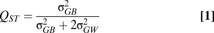Here, is the additive genetic variance between populations, which is usually estimated in a common garden environment (17), and is the additive genetic variance within populations, which is estimated using information on relatedness of individuals. An assumption of the method is that all genetic variance is attributable to additive effects. Q_ST = 0 corresponds to a situation in which all the genetic variation is found within rather than between populations. Q_ST = 1 corresponds to a situation in which genetic differences exist among populations but all individuals are genetically identical with respect to the trait within a population.

Q_ST can be compared with F_ST estimates. If Q_ST is significantly greater than F_ST, a pure drift model of trait divergence is rejected and a role for divergent selection is invoked (16). A logistic challenge in estimating Q_ST is the requirement for common garden experiments and information on the relatedness of individuals. In many instances, only phenotypic data are available; in such case, an estimate of Q_ST can be obtained using its phenotypic equivalent, P_ST (18, Eq. 2):

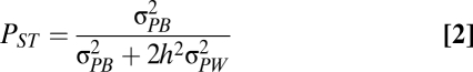Here, h² is the narrow-sense heritability and and are the phenotypic variances across and within populations, respectively. The degree to which P_ST provides a good estimate of Q_ST depends on (i) the accuracy of the heritability estimate and (ii) the degree to which differences between populations are genetic. Large P_ST values may arise if phenotypic differences between populations are actually environmental in origin because is an upwardly biased estimator of (19).

We have developed a technique that distinguishes between-population genetic differences from environmental differences using phenotypic and environmental (in the case considered here, temperature) data that vary over time and space. Eq. 3 describes variation in mean phenotype (in the case considered here, first spawning date, y) measured for a set of individuals belonging to year i in population j. In this case, and is the deviation of population j from the grand mean attributable to additive effects and differences in environment, respectively. and ε_ij is the deviation of a set of individuals belonging to year i from the mean of population j attributable to the average annual breeding value and the environment, respectively:

The aim of Q_ST is to compare variation in with α. In the absence of transplant experiments, and are confounded. The paucity of prior information for many traits often leads studies to make the assumption that = 0. In the absence of pedigree information, α and ε are confounded.

Here, we introduce the variables (indicating the mean temperature experienced by population j) and (indicating the deviation in temperature from the mean of population j that individuals in year i experience). We assume that the effect temperature has on phenotype (β) is consistent for all individuals irrespective of the population they belong to (Eq. 4), which is equivalent to assuming that mean population plasticity with respect to temperature is constant within and among populations. The environmental effects ( and ) are now deviations after correcting for the effects of temperature:

Let G and E denote additive genetic effects and environmental effects, respectively. Under this model, the expected variances (σ²) and covariances (σ) between temperature (T) and phenotype (Y) within (W) and between (B) populations are equal to:

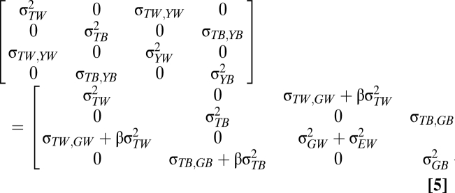Given Eq. 5, the difference between the between- and within-population slopes is given by:

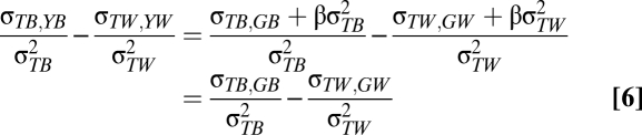Thus, Eq. 6 gives an estimate of the genetic differentiation between populations (i.e., local adaptation) compared with that within populations (i.e., microevolution through time) with respect to temperature. We propose that if the between- and within-population slopes are not significantly different, this would be consistent with the hypothesis that phenotypic differences between populations are the result of mean plasticity alone (Fig. 1A). Alternatively, if the slopes do differ significantly, this suggests that population phenotypes show local adaptation (Fig. 1 B–D depicts three such scenarios and their biological interpretations).

Fig. 1.

Schematic of within- (dotted lines) and between- (solid lines) population temperature × first spawning date covariation. (A) Within- and between-population slopes are the same. Negative covariation within populations could arise via mean plasticity and/or microevolution (with mean plasticity as the null hypothesis), and negative covariation between populations could arise via mean plasticity and/or local adaptation (with mean plasticity as the null hypothesis). (B) There is no covariation within populations but negative covariation between populations; therefore, slopes differ. The between-population covariation is consistent with local adaptation. (C) There is negative covariation within populations and orthogonal positive covariation between populations; therefore, slopes differ. The within-population covariation is consistent with maladaptive mean plasticity, and the between-population covariation is consistent with local adaptation. (D) There is negative covariation within populations but no covariation between populations; therefore, slopes differ. This pattern would be consistent with maladaptive mean plasticity within populations and local adaptation counteracting this effect between populations [i.e., countergradient variation (45)].

Results and Discussion

We compared the within-population (across years) and between-population slopes for temperature vs. R. temporaria first spawning dates using >50,000 observations from across Britain spanning the period 1998–2006. We used a bivariate mixed model framework, wherein temperature and spawning date were both response variables.

Across space and time, mean January temperature correlated more strongly with spawning dates than did several other winter temperature variables, as revealed by higher pseudo-R² values when comparing models that include comparable random effects (Fig. 2 and Table S1). The bivariate mixed model with the lowest deviance information criterion (DIC) included five random terms: year, 150-km grid-square, 50-km grid-square, and the two interactions between these grid-squares and year. The space-by-time interactions were fitted to allow for year-to-year variation that was specific to spatial locations. For each random term, we estimated a variance component for temperature, spawning date, and the covariance between the two. Dividing the covariance by the temperature variance component defines a regression slope for each random effect (20).

Fig. 2.

Relation between maximum January temperatures and frog first spawning dates in Julian days across 150-km population means, where each data point corresponds to a single population mean (calculated as the mean of the yearly means) (A), and within 150-km populations through time, where each data point corresponds to an annual population mean in a single grid-square (B). Lines correspond to least squares regression estimates. Only populations with data for at least 5 years were included. Green, northern populations (UKCP09 grid-square ID 1–702); blue, midlatitude populations (grid-square ID 703–1638); red, southern populations (grid-square ID >1638).

In all cases, the slopes between temperature and first spawning date were negative: 150-km slope (b) = −12.91, 95% highest posterior density (HPD): −16.82 to −9.61; 50-km b = −5.10, HPD: −6.91 to −2.92; year b = −3.25, HPD: −7.29–1.41; year/150-km b = −3.44, HPD = −4.89 to −2.17; year/50-km b = −2.61, HPD: −5.52–0.05; residual b = −1.67, HPD: −1.92 to −1.43. We consider the contribution of microevolution to the within-population temporal slope ( in Eq. 6) to be minimal because the directional temperature change over the 9-year duration of this study was slight (January mean temperature b = 0.05 ± 0.02, February mean temperature b = −0.20 ± 0.02) (21) and R. temporaria requires 2 or 3 years to reach sexual maturity (22). Therefore, terms involving year reflect plastic responses to temperature and are not significantly different from each other (pooled mean = −2.98, HPD: −4.84 to −1.33).

Terms not involving year (including the residual) capture the combined effects of mean population plasticity and local adaptation. The difference between the temporal slopes and the spatial slopes therefore quantifies temperature-related local adaptation. There is no evidence for local adaptation within 50-km grid-squares (slope difference (Δb) = 1.26, HPD: −0.36–3.22), weak evidence within 150-km grid-squares (Δb = −1.99, HPD: −4.30–1.03), but strong evidence between 150-km grid-squares (Δb = −10.03, HPD: −14.04 to −5.99) (Fig. 2). The observed within 150-km and between 150-km population slopes are intermediate between the relations depicted in Fig. 1 A and B. We can also infer that the mean plasticity exhibited by populations is adaptive on the grounds that the within-population and between-population slopes are of the same sign. All the main conclusions are consistent under alternative tests and across different models that include minimum, mean, and maximum January and February temperatures, each of which is considered in 10 mixed effects models with different random effect combinations (total of 60 models; Table S1).

The number of spawning date observations is highly heterogeneous over both space and time (Fig. S1), with there being many more observations in southern Britain than further north. Our slope estimates will be weighted toward those observed in southern parts of Britain if heterogeneity exists. However, we think this bias is unlikely to undermine the observed difference in slopes, given that the results are qualitatively unchanged when each grid-cell only contributes a single data point across multiple years for the calculation of the between-population slope (Fig. 2A) and when each year only contributes a single data point per grid-cell for the calculation of the within-population slope (Fig. 2B).

Our model (Eq. 4) assumes that the slopes are constant across different units within a random effect, but several studies have reported heterogeneity of within-population slopes across different populations (23). Although we find a small but significant degree of heterogeneity when comparing within 150-km population slopes, we are cautious as to whether this variance is real or attributable to variation in the number of observations across grid-cells and years (Methods).

The large effect size of local adaptation is best illustrated by example. Consider the 150-km grid-squares covering southwest Britain (mean January temperature = 5.96 °C, mean first spawning date = 37.1 Julian days) and northeast Britain (mean January temperature = 3.16 °C, mean first spawning date = 78.9 Julian days). If individuals from the northeast were translocated to the southwest, we predict that their mean first spawning date would advance by 8.3 days because of plasticity. However, this would still leave them spawning 33.5 days later than the resident population, which is locally adapted to the average temperature of its grid-square. Although we find stronger evidence for local adaptation at a large spatial scale (between 150-km grid-squares) than we do at a smaller scale (between 50-km grid-squares), local adaptation is unlikely to be a threshold process and presumably accumulates over distance as the ameliorating effects of gene flow diminish.

One explanation for shallower within-population slopes than between-population slopes relates to a combined effect of an individual's prediction and regression to the mean. If within-population within-year temporal autocorrelation in temperatures is low, then extreme January temperatures are less reliable than within-population multiyear averages at predicting the temperature in following months. Consequently, an adaptive response to temperature may be more optimal if it tracks multiyear averages rather than transient temporal fluctuations. This is consistent with the fact that southerly populations spawn earlier than northern populations when they experience the same January temperatures. Although such a process could give rise to differences in slope through local adaptation, it is possible that older frogs use a cumulative multiyear prediction of temperature to achieve the same ends (24).

By combining our slope estimates with UK Climate Impacts Programme January mean temperature change projections for grid-squares in Britain across the period 2050–2070 (25), we can map the projected advance in spawning date expected via plasticity alone (the product of the pooled mean temporal slope and temperature increase; Fig. 3A) and the advance necessary for a population to be as locally adapted as contemporary populations (the product of the between 150-km population slope and temperature increase; Fig. 3B). Projected temperature increases for the period 2050–2070 are highest in the southeast (up to 3.0 °C) and considerably less in the far northwest (<1.7 °C). As a consequence, population plasticity is projected to lead to the greatest advances in southeast Britain and the smallest advances in the northwest (Fig. 3A). The advance required for populations to remain as locally adapted as contemporary populations shows the same geographical pattern (Fig. 3B). We can map the shortfall between the advance required for populations to remain locally adapted and the advance expected via plasticity alone (Fig. 3C). This shortfall could exceed 25 days in southeast Britain. However, in light of evidence for nonlinearities in the temperature vs. spawning date relation across Europe (26), there is a need for caution in interpreting extrapolations beyond the range of the current observations.

Fig. 3.

Map of geographical variation in projected advance of first spawning date via plasticity, temperature increase × within-population slope of 2.98 (A); necessary advance for populations to be as locally adapted as contemporary populations, temperature increase × between 150-km population slope of 12.91 (B); and the microevolution and gene-flow challenge (C), the difference between the necessary advance for populations to be as locally adapted as contemporary populations (B) and advance expected via plasticity alone (A). Slope estimates come from the best model. Median January temperature increase projections for the period 2050–2070 on a 25 × 25-km grid come from the UK Climate Impacts Programme (further details are provided in Methods).

The fitness consequences of a shortfall in advance are not known and represent a priority for future experimental work. Laboratory studies on the developmental times of amphibian embryos have shown that high-latitude populations are sometimes adapted to temperatures above those that they routinely encounter in the wild (27). This is perhaps attributable to natural selection not keeping pace with postglacial geographical expansion from lower latitudes. If this were the case, it would represent the best case scenario for British R. temporaria, meaning that local populations may not incur direct fitness costs from the projected temperature increases. However, an alternative explanation for these laboratory findings may be that amphibians are prevented from developing at their optimum temperature in the wild by other factors such as predation pressure and competition. Assuming that a rise in temperature leads to direct selection for earlier spawning in R. temporaria populations, the short-term evolutionary response will largely depend on the standing genetic variation for spawning date within current populations (20) and the rate of northward gene flow from populations adapted to higher average temperatures (24, 28).

A matter of concern is that local adaptation in spawning date and other life history traits in R. temporaria (e.g., 12) implies that levels of gene flow may be low. Strong selection pressures may lead to population declines unless evolution can keep pace with the rate of environmental change (24, 29) or efforts to reverse habitat fragmentation and increase landscape permeability are sufficient to increase the frequency of long-distance dispersal.

Within Britain, southeastern populations face the greatest expected change in temperature and, therefore, the strongest microevolutionary and gene flow challenge (Fig. 3C). This raises two concerns. First, these populations are likely to have less opportunity for natural immigration from further south, because of the proximity of the English Channel, than are northern populations. Second, the high levels of urbanization in southeast Britain may further restrict gene flow in this species (30), although this may be countered by the abundance of small ponds in urban areas (31).

Amphibians are experiencing rapid global declines (32, 33). Thermal tolerances of high-latitude amphibians are typically broader than among their tropical counterparts, and it has been suggested that they are likely to be less adversely affected by climate change (3). Given that the common frog is a widespread species, our data suggest that other amphibians at high latitudes may also find rapid climate change challenging.

Our results raise issues about the validity of the “space-for-time” substitution approach often employed in studies in which spatial replication is possible but temporal replication is not (34–36). If, in the absence of knowledge of the temporal relation between temperature and phenology in R. temporaria, the spatial relation was used to predict the temporal relation, the prediction would have the correct sign but would lead to a substantial overestimate of the short-term temporal slope. If, however, the space-for-time substitution was applied to a case in which the difference between the spatial and temporal relations was more pronounced, this could, in extreme cases (e.g., Fig. 1C), lead to the sign being incorrectly predicted. Thus, we recommend exercising caution in the application of space-for-time substitutions to intraspecific phenotypic variation, especially if local adaptation is suspected.

Methods

Data.

The UK Phenology Network (UKPN; www.naturescalender.org.uk) has collated public observations of first spawning dates for R. temporaria across Britain. Observations of spawning dates that occurred after 200 Julian days (n = 108) and in Northern Ireland were excluded from the analysis, leaving 55,602 observations. We matched the remaining observations with January and February minimum, mean, and maximum temperatures from 1998 to 2006, interpolated to the nearest 5-km square on a rotated latitude projection (grid North Pole longitude = 198.0, grid North Pole latitude = 39.25) (37). The raw monthly gridded climate data, which form part of the UK climate projections (UKCP09) data, were obtained from the UK Met Office (http://www.metoffice.gov.uk/climatechange/science/monitoring/ukcp09/).

We divided the United Kingdom into grid-squares, or “populations,” at 50 × 50-km, 100 × 100-km, and 150 × 150-km resolutions (mean spawning date per 25-km grid-cell per year, and the number of observations can be obtained at http://www.naturescalendar.org.uk/findings/research_archive.htm).

Temperature Trend.

We tested for directional temperature change over the 9 years of this study using a linear mixed effects model with population as a random effect and year as a continuous fixed effect. Models were fitted using the lme4 R library. We assumed that the January/February temperatures in a location over the period 1998–2006 correlate with historic average January/February temperatures [since the last glacial maxima, ≈20,000 years ago (38)].

Slope Test.

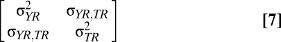
We used a Markov chain Monte Carlo approach to fit Bayesian generalized linear mixed models (39) to the entire dataset. Models were run for 13,000 iterations with a burn-in of 3,000 iterations, a thinning interval of 10 and flat priors. We fitted temperature and first spawning date as a bivariate normal response and population, year, and their interaction as random effects. Some analyses included a nested sequence of population level random effects (e.g., 50 × 50-km grid-squares within 150 × 150-km grid-squares). For each random effect, the variance covariance matrix was estimated (Eq. 7), where Y is first spawning date, T is temperature, and R denotes the random effect:

Slopes were estimated as . The 95% highest posterior densities of the slopes and the difference between slopes (Δb) were estimated and used to assess whether slopes differed from zero and from each other, respectively.

In Eq. 8, we define a pseudo-R² for the model across k random effects (R):

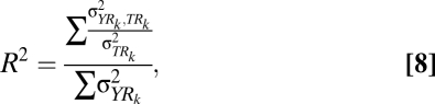which measures the expected proportion of variation explained rather than the actual proportion explained. Model fit was assessed using the DIC and pseudo-R².

Being correlational, our approach is sensitive to the influence of third variables. For example, a variable that correlates with temperature and spawning date to a differing degree over space and time would generate a difference in slopes that could be misinterpreted as evidence of local adaptation. When such third variables are known, they can be included in the statistical model either as fixed effects or as additional response variables. The approach described here does not correct for spatial or temporal autocorrelation, which may lead to underestimation of the true confidence intervals for between-population and within-population slopes, respectively.

Recent studies have emphasized the importance of considering environment by phenology correlations at multiple trophic levels (40, 41). Our statistical approach can be extended to include the phenology of multiple species as separate response variables. For each random effect, this would allow the estimation of a temperature-by-phenology slope for every species plus the phenology_A-by-phenology_B slope between species A and B at different trophic levels.

Within-Population Slope Heterogeneity.

To allow for within-population slope heterogeneity, it would be necessary to let the covariance matrices within each population vary as additional levels in the multilevel model, making this very difficult to implement. Random regression is often used to test for heterogeneity in slopes but cannot be applied in this case because of the within-population and between-population slopes differing.

As shown in Eq. 9, if we only allow for populations defined by 150 × 150-km grid-squares, then an appropriate model incorporating heterogeneous within population slopes would be:

where μ is the intercept and is the deviation of the mean phenotype in population j from the grand mean. is the between-population slope, is the expected within 150-km population slope, and is the deviation of the within-population slope for population j from the expected within-population slope.

The problem is that neither t nor τ is known and so must be estimated, as they are in the bivariate model. An alternative, which is shown in Eq. 10 but which we are reluctant to advocate, is to decompose each temperature into the observed mean and a deviation (42), essentially fitting the model:

where d is the deviation between the mean of the sample and the true hypothetical mean. The hats on the model parameters indicate that they are only identical to the original parameters when d = 0. In the extreme case, when there is only a single datum within population j, then . Eq. 10 can be rearranged as shown in Eq. 11:

which makes it clear that variation in d could result in biased estimates of all slope parameters. In this sense, the multivariate mixed model that we used is to be preferred because it correctly weights random effects by the information present within and between levels. Nonetheless, as a diagnostic test, we estimated the parameters of the model using flat priors and the full (co)variance matrix for the random intercepts and slopes. This model suggested that slope variation did exist within populations 1.546 (0.884–4.206), but the difference between within-population and between-population slopes remained qualitatively unchanged Δb = −9.061 (−12.734 to −5.253).

When we fitted the interaction between the mean latitude of observations in a grid-cell and the within-population slope, there was a significant tendency for more northerly populations to have shallower reaction norms (posterior mode = 0.366, HPD: 0.109–0.635). This corresponds to the within-population slope varying from −4.76 in the south to −0.995 in the north. However, we are reluctant to ascribe biological significance to the observed latitudinal variation in the within-population slope because the bias introduced by d_j is likely to increase with latitude (Fig. S1).

Measurement Error.

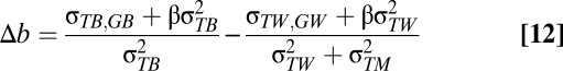
Measurement error in temperature will reduce the magnitude of the slope for those levels in which the measurement error is introduced. In the context of this study, this would be a problem if measurement error occurs within populations. We can adapt Eq. 6 to see how much measurement error in temperature () would need to exist to generate the slope difference (Δb) that we find, as shown in Eqs. 12–14:

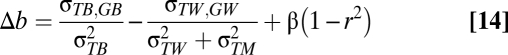If we assume an absence of microevolution, the covariance between temperature and breeding value within populations is zero. However, the difference in slopes is still downwardly biased by β(1−r²) assuming that β is negative. The repeatability of the temperatures is represented by r². In Eq. 15 we assume that local adaptation is also absent, so:

Under this scenario, the between-population slope is an unbiased estimator of β because measurement error in temperatures occurs within populations. Because we found this slope to be −12.91 and the difference to be −10.03, as shown in Eqs. 16 and 17, then:

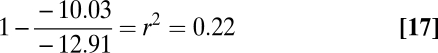Therefore, the repeatability would have to be unreasonably low (<0.23), for the conclusions of this paper to be compromised. However, the low-slope estimate within 50-km grid-squares may be attributable to measurement error in local interpolated temperature estimates, which will cause the temperature vs. spawning date slope to be underestimated.

Projecting Spawning Advance.

We obtained 50% quantile projections of mean January temperature increase for 2050–2070 in 25 × 25-km grid-squares from UKCP09 Bayesian posterior distributions (25) corresponding to the Intergovernmental Panel for Climate Change Special Report on Emissions Scenarios A1F1 (fossil fuel intensive) scenario (43). These temperature projections were combined with within- and between-population slope estimates to map the (i) projected advance attributable to plasticity, (ii) projected advance in local optima, and (iii) projected shortfall between plastic advance and local optima. All statistical analyses were conducted in R (44).

References

- 1.Mayr E. Animal Species and Evolution. Cambridge, MA: Harvard Univ Press; 1963. [Google Scholar]
- 2.Endler JA. Geographic Variation, Speciation, and Clines. Princeton: Princeton Univ Press; 1977. [PubMed] [Google Scholar]
- 3.Deutsch CA, et al. Impacts of climate warming on terrestrial ectotherms across latitude. Proc Natl Acad Sci USA. 2008;105:6668–6672. doi: 10.1073/pnas.0709472105. [DOI] [PMC free article] [PubMed] [Google Scholar]
- 4.Davis M, Shaw R. Range shifts and adaptive responses to Quaternary climate change. Science. 2001;292:673–679. doi: 10.1126/science.292.5517.673. [DOI] [PubMed] [Google Scholar]
- 5.Kawecki TJ, Ebert D. Conceptual issues in local adaptation. Ecol Lett. 2004;7:1225–1241. [Google Scholar]
- 6.Beebee TJC. Amphibian breeding and climate. Nature. 1995;374:219–220. [Google Scholar]
- 7.Loman J. Primary and secondary phenology. Does it pay a frog to spawn early? J Zool. 2009;279:64–70. [Google Scholar]
- 8.Walther G-R, et al. Ecological responses to recent climate change. Nature. 2002;416:389–395. doi: 10.1038/416389a. [DOI] [PubMed] [Google Scholar]
- 9.Beattie RC, Ashton RJ, Milner AGP. A field study of fertilization and embryonic development in the common frog (Rana temporaria) with particular reference to acidity and temperature. Journal of Applied Ecology. 1991;28:346–357. [Google Scholar]
- 10.Carroll EA, Sparks TH, Collinson N, Beebee TJC. Influence of temperature on the spatial distribution of first spawning dates of the common frog (Rana temporaria) in the UK. Global Change Biology. 2009;15:467–473. [Google Scholar]
- 11.Gienapp P, Teplitsky C, Alho JS, Mills JA, Merila J. Climate change and evolution: Disentangling environmental and genetic responses. Mol Ecol. 2008;17:167–178. doi: 10.1111/j.1365-294X.2007.03413.x. [DOI] [PubMed] [Google Scholar]
- 12.Laugen AT, Laurila A, Rasanen K, Merila J. Latitudinal countergradient variation in the common frog (Rana temporaria) development rates—Evidence for local adaptation. J Evol Biol. 2003;16:996–1005. doi: 10.1046/j.1420-9101.2003.00560.x. [DOI] [PubMed] [Google Scholar]
- 13.Palo JU, et al. Latitudinal divergence of common frog (Rana temporaria) life history traits by natural selection: Evidence from a comparison of molecular and quantitative genetic data. Mol Ecol. 2003;12:1963–1978. doi: 10.1046/j.1365-294x.2003.01865.x. [DOI] [PubMed] [Google Scholar]
- 14.Lande R. Statistical tests for natural-selection on quantitative characters. Evolution. 1977;31:442–444. doi: 10.1111/j.1558-5646.1977.tb01025.x. [DOI] [PubMed] [Google Scholar]
- 15.Turelli M, Gillespie JH, Lande R. Rate tests for selection on quantitative characters during macroevolution and microevolution. Evolution. 1988;42:1085–1089. doi: 10.1111/j.1558-5646.1988.tb02526.x. [DOI] [PubMed] [Google Scholar]
- 16.Spitze K. Population-structure in Dapnia obtusa: Quantitative genetic and allozymic variation. Genetics. 1993;135:367–374. doi: 10.1093/genetics/135.2.367. [DOI] [PMC free article] [PubMed] [Google Scholar]
- 17.Merilä J, Crnokrak P. Comparison of genetic differentiation at marker loci and quantitative traits. J Evol Biol. 2001;14:892–903. [Google Scholar]
- 18.Leinonen T, Cano JM, Makinen H, Merila J. Contrasting patterns of body shape and neutral genetic divergence in marine and lake populations of threespine sticklebacks. J Evol Biol. 2006;19:1803–1812. doi: 10.1111/j.1420-9101.2006.01182.x. [DOI] [PubMed] [Google Scholar]
- 19.Whitlock MC. Evolutionary inference from QST. Mol Ecol. 2008;17:1885–1896. doi: 10.1111/j.1365-294X.2008.03712.x. [DOI] [PubMed] [Google Scholar]
- 20.Falconer DS, MacKay TFC. Introduction to Quantitative Genetics. 4th Ed. Essex: Longman; 1996. Harlow, Essex, UK. [Google Scholar]
- 21.Knight J, et al. Do global temperature trends over the last decade falsify climate predictions? Bulletin of the American Meteorological Society. 2009;90:S1–S196. [Google Scholar]
- 22.Miaud C, Guyetant R, Elmberg J. Variations in life-history traits in the common frog Rana temporaria (Amphibia: Anura): A literature review and new data from the French Alps. Journal of Zoological Society of London. 1999;249:61–73. [Google Scholar]
- 23.Liefting M, Hoffmann AA, Ellers J. Plasticity versus environmental canalization: Population differences in thermal responses along a latitudinal gradient in Drosophila serrata. Evolution. 2009;63:1954–1963. doi: 10.1111/j.1558-5646.2009.00683.x. [DOI] [PubMed] [Google Scholar]
- 24.Visser ME. Keeping up with a warming world; Assessing the rate of adaptation to climate change. Proc R Soc London Ser B. 2008;275:649–659. doi: 10.1098/rspb.2007.0997. [DOI] [PMC free article] [PubMed] [Google Scholar]
- 25.Murphy JM, et al. A methodology for probabilistic predictions of regional climate change from perturbed physics ensembles. Philosophical Transactions of the Royal Society A: Mathematical, Physical and Engineering Sciences. 2007;365:1993–2028. doi: 10.1098/rsta.2007.2077. [DOI] [PubMed] [Google Scholar]
- 26.Sparks TH, Tryjanowski P, Cooke A, Crick H, Kuzniak S. Vertebrate phenology at similar latitudes: Temperature responses differ between Poland and the United Kingdom. Climate Research. 2007;34:93–98. [Google Scholar]
- 27.Bachmann K. Temperature adaptations of amphibian embryos. Am Nat. 1969;103:115–130. [Google Scholar]
- 28.Bridle JR, Vines T. Limits to evolution at range margins: When and why does adaptation fail? Trends Ecol Evol. 2007;22:140–147. doi: 10.1016/j.tree.2006.11.002. [DOI] [PubMed] [Google Scholar]
- 29.Ludwig GX, et al. Short- and long-term population dynamical consequences of asymmetric climate change in black grouse. Proc Royal Soc London Ser B. 2006;273:2009–2016. doi: 10.1098/rspb.2006.3538. [DOI] [PMC free article] [PubMed] [Google Scholar]
- 30.Hitchings SP, Beebee TJC. Genetic substructuring as a result of barriers to gene flow in urban Rana temporaria (common frog) populations: Implications for biodiversity conservation. Heredity. 1997;79:117–127. doi: 10.1038/hdy.1997.134. [DOI] [PubMed] [Google Scholar]
- 31.Gaston KJ, Warren PH, Thompson K, Smith RM. Urban domestic gardens (IV): The extent of the resource and its associated features. Biodiversity and Conservation. 2005;14:3327–3349. [Google Scholar]
- 32.Houlahan JE, Findlay CS, Scmidt BR, Meyer AH, Kuzmin SL. Quantitative evidence for global amphibian population declines. Nature. 2000;404:752–755. doi: 10.1038/35008052. [DOI] [PubMed] [Google Scholar]
- 33.Stuart SN, et al. Status and trends of amphibian declines and extinctions worldwide. Science. 2004;306:1783–1786. doi: 10.1126/science.1103538. [DOI] [PubMed] [Google Scholar]
- 34.Fukami T, Wardle DA. Long-term ecological dynamics: Reciprocal insights from natural and anthropogenic gradients. Proc R Soc London Ser B. 2005;272:2105–2115. doi: 10.1098/rspb.2005.3277. [DOI] [PMC free article] [PubMed] [Google Scholar]
- 35.Pickett STA. Space-for-time substitution as an alternative. In: Likens GE, editor. Long-Term Studies in Ecology: Approaches and Alternatives. New York: Springer; 1989. pp. 110–135. [Google Scholar]
- 36.La Sorte FA, Lee TM, Wilman H, Jetz W. Disparities between observed and predicted impacts of climate change on winter bird assemblages. Proc R Soc London Ser B. 2009;276:3167–3174. doi: 10.1098/rspb.2009.0162. [DOI] [PMC free article] [PubMed] [Google Scholar]
- 37.Perry M, Hollis D. The generation of monthly gridded datasets for a range of climatic variables over the UK. International Journal of Climatology. 2005;25:1041–1054. [Google Scholar]
- 38.Clark CD, Gibbard PL, Rose J. Pleistocene glacial limits in England, Scotland and Wales. In: Ehlers J, Gibbard PL, editors. Quaternary Glaciations—Extent and Chronology. Amsterdam: Elsevier; 2004. pp. 47–82. [Google Scholar]
- 39.Hadfield JD. MCMC methods for multi-response generalized linear mixed models: The MCMCglmm R package. Journal of Statistical Software. 2010;33:1–22. [Google Scholar]
- 40.Visser ME, Both C. Shifts in phenology due to global climate change: The need for a yardstick. Proc R Soc London Ser B. 2005;272:2561–2569. doi: 10.1098/rspb.2005.3356. [DOI] [PMC free article] [PubMed] [Google Scholar]
- 41.Thackeray SJ, et al. Trophic level imbalances in rates of phenological change for marine, freshwater and terrestrial environments. Global Change Biology. 2010 in press. [Google Scholar]
- 42.van de Pol M, Wright J. A simple method for distinguishing within- versus between-subject effects using mixed models. Anim Behav. 2009;77:753–758. [Google Scholar]
- 43.Nakicenovic N, et al. Special Report on Emissions Scenarios. Cambridge, UK: Cambridge University Press; 2000. p. 598. [Google Scholar]
- 44.R Development Core Team R: A language and environment for statistical computing (R Foundation for Statistical Computing, Vienna) 2009. Available at http://www.R-project.org.
- 45.Conover DO, Schulz ET. Phenotypic similarity and the evolutionary significance of countergradient variation. Trends Ecol Evol. 1995;10:248–252. doi: 10.1016/S0169-5347(00)89081-3. [DOI] [PubMed] [Google Scholar]
Associated Data
This section collects any data citations, data availability statements, or supplementary materials included in this article.