Identifying the dynamics of complex spatio-temporal systems by spatial recurrence properties

Abstract

Complex spatio-temporal systems may exhibit irregular behaviors when driven far from equilibrium. Reaction-diffusion systems often lead to the formation of patterns and spatio-temporal chaos. When a limited number of observations is available, the reconstruction and identification of complex dynamical regimes become challenging problems. A method based on spatial recurrence properties is proposed to deal with this problem: generalized recurrence plots and generalized recurrence quantification analysis are exploited to show that detection of structural changes in spatially distributed systems can be performed by setting up appropriate diagrams accounting for different spatial recurrences. The method has been tested on two prototypical systems forming complex patterns: the complex Ginzburg–Landau equation and the Schnakenberg system. This work allowed us to identify changes in the stability of spiral wave solutions in the former system and to analyze the Turing bifurcations in the latter.

Reaction-diffusion equations are widely used for modeling a large variety of observed natural and physico-chemical spatial phenomena, such as chemical reactions (1), biological systems and population dynamics (2), and pattern formation in physical systems (3, 4). In fact, when driven outside from equilibrium, spatially extended systems may exhibit irregular behavior both in space and time. This phenomenon, commonly known as spatio-temporal chaos (5, 6), consists in the spontaneous emergence of spatial patterns like Turing structures, traveling and spiral waves, and turbulence. Reaction and diffusion have been widely investigated both from the theoretical (7, 8, 9) and experimental viewpoints (10).

One important and still open issue arises in studying an unknown dynamical spatio-temporal system when only the observation of one or a part of its spatial variables (or a combination of them) is known and observation data is poorly available. The problem of space-state reconstruction and model identification of a spatio-temporal dynamical system has been investigated in lattice dynamical systems (11), whereas a method for spatial forecasting from single snapshots has been proposed in (12). In such cases one has to cope with the problem of understanding the dynamics of a system by using only a limited amount of data.

This paper attempts to provide a methodology for extracting information on the dynamics of a distributed dynamical system from a limited number of spatial observations and, in particular, for detecting structural changes in its dynamics.

Discussion

Spatial Recurrence Strategies.

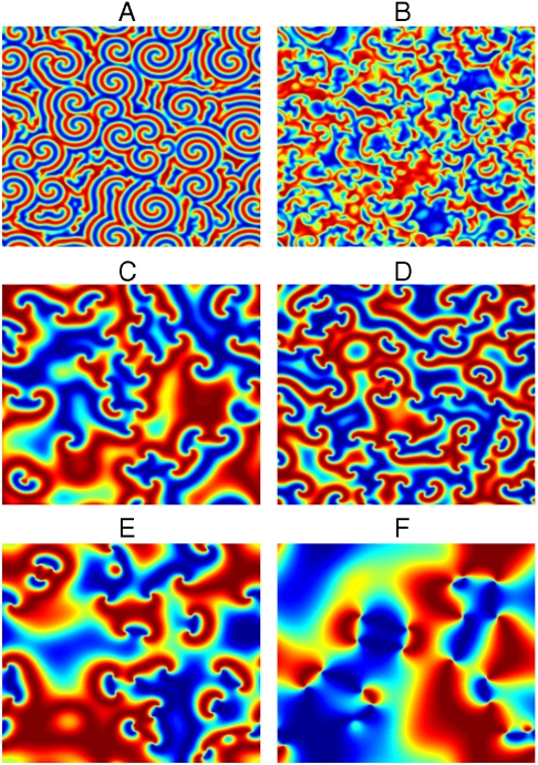
Let us consider the images shown in Fig. 1. We may consider these images as snapshots of an unknown two-dimensional system, and we want to extract as much information as possible about the underlying system. Indeed, they represent the numerical solutions at equal times of a spatially distributed system (which will be described later) for different values of its characteristic parameters. One can notice that some images have similar patterns, whereas others are substantially different.

Fig. 1.

Patterns obtained by the system of Eq. 1 for different values of the parameters (α,β).

Of course, the solution of the inverse problem is a formidable task, which cannot be solved in general, except in very special cases. For this reason, we focus on a more limited scope: to devise a systematic methodology based on experimental data to detect changes in the system dynamics and in its qualitative behavior.

We start by considering that the formation of a pattern in a certain region depends on the spatio-temporal dynamics of the system. Hence, spatial state recurrences may give insight in the evolution of the system.

Indeed, the concept of recurrence is strictly related to that of dynamical systems, as originally stated by Poincaré. For time series, temporal recurrence of states has been widely investigated by means of recurrence plots and recurrence quantification analysis (13), whereas the problem of spatial recurrence in biomedical images was investigated by Marwan et al. (14), who developed the generalization for spatial systems, leading to generalized recurrence plots (GRP) and generalized recurrence quantification analysis (GRQA) (see Materials and Methods for details).

Recently, the authors of this paper proposed the use of GRP and GRQA for the analysis of spatially distributed systems by introducing the determinism-entropy (D-E) diagram, a tool accounting for the recurrence properties of images generated by a dynamical system (15). In this paper, we intend to go beyond this task and answer the following question: Is this framework capable of extracting all the useful information from a sequence of images for detecting structural changes in the dynamics of the generating system?

Following ref. 15, determinism is an appropriate measure accounting for the global structure of the image, whereas entropy represents a measure accounting for the patterns at small scales. In fact, the combination of both indicators in the determinism-entropy diagram provides a suitable description of the image at micro and macro scales. Table 1 reports the values of both indicators for the images of Fig. 1. One can notice that D ranges approximately from 10.6 to 27.5 and E from 1.8 to 3.2. We observe that the points corresponding to the pair (a),(b) are quite close in the D-E plane. The same holds for the pair (e),(f), whereas the pair (c),(d) shows values different from the other two pairs and in addition (c) is somewhat far from (d). Such differences may be related to structural changes (see ref. 16 for similar behavior in one dimensional systems). The hypothesis of abrupt changes in the recurrence indicators is consistent with the nature of the system used to generate the patterns; i.e., the Complex Ginzburg–Landau Equation (CGLE)

[1]

where , x, y are the spatial variables and (17, 18). This is one of the most important and studied nonlinear partial differential equations describing pattern formation in a spatially distributed system near a Hopf bifurcation. The interest in Ginzburg–Landau equations has been sustained because its solutions display a very rich spectrum of dynamical behaviors when the parameters are varied. This allows one to describe a large variety of physical systems, such as nonlinear waves, second order phase transitions, superconductivity and superfluidity, Bose–Einstein condensation and population dynamics (19). An important feature of the CGLE is the structure, nature, and role of defects, i.e. points in the space where |A| = 0. For two-dimensional systems, defects are points that appear and disappear in pairs, and, for small enough values of α, they are able to generate (stable or unstable) spiral waves (further details in Materials and Methods). The behavior of the solution in the parameter space (α,β) is very complex and still under investigation.

Table 1.

Values of D and E of the images in Fig. 1

	(a)	(b)	(c)	(d)	(e)	(f)
D	10.62	11.26	21.14	16.70	27.48	26.14
E	1.834	1.797	2.625	2.116	3.013	3.202

To give an answer to the problem posed at the beginning of this section, in the following we present a methodology based on recurrence properties of the images for a detailed analysis of the CGLE and reaction-diffusion systems.

Detection of Structural Changes.

The behavior of the CGLE in the plane (α,β) has been extensively studied by Huber (17, 20, 21), Brito (22), and Chaté and Manneville (23, 24). On the basis of extensive simulations, they define a set of transition lines in the region β > 0. In particular, they identify the convective instability limit, the absolute instability limit, and the regions in which the phase turbulence and defect turbulence are observed.

In our investigation, a systematic analysis of the CGLE has been performed in a square domain of the parameter space α × β = [-1.5,1.5] × [-1.5,1.5]^*. The parameter plane has been sampled by varying α by steps of 0.25, and β of 0.1. Specifically, the real part of solutions A(x,y) of the CGLE has been considered for each pair (α_i,β_i).

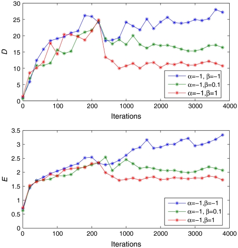
To guarantee the stationarity of the measures, we first look at the temporal evolution of both determinism and entropy starting from random initial conditions. Fig. 2 shows the dynamics of D for α = -1 and β∈{-1,0.1,1}. For each β, D reaches a different saturation value, after the transient. For E the same behavior has been observed. This analysis allows for the selection of an appropriate stopping time for the integration and guarantees the stationarity of both D and E.

Fig. 2.

Analysis of the CGLE patterns. Time evolution of D and E for α = -1.0 and β∈{-1,0.1,1} and random initial conditions. After the transient time (approximately 1500 iterations), both D and E reach a stationary value. This allows for a proper selection of the integration stopping time to avoid biased values of determinism and entropy due to transient behavior.

A preliminary information on the variation of the GRQA measures with respect to β is obtained by introducing a sensitivity indicator defined by

[2]

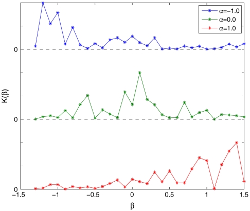
where and are the averages of entropy and determinism, respectively. A small value of K(β) indicates that both E and D do not vary significantly with β. Fig. 3 reports K(β) for three different values of α: One can notice that, depending on α and β, the three curves show two clearly distinct behaviors characterized by low and high sensitivity.

Fig. 3.

Sensitivity function K(β) for α∈{-1,0,1} and β∈[-1.5,1.5]. The curves are shifted along the y axis for the sake of readability. High values of K(β) point out that small variations of β may produce significant variations in the values of determinism and entropy.

High values of K(β) point out that small variations of β may produce strongly different patterns: This variability is related to the position and number of defects, allowing for the formation of structures with different spatial distribution. This is consistent with the fact that defects arise, collide, and annihilate in the unstable wave solution case. On the contrary, in the stable case, the number and location of defects is robust to small variations of the parameter β, giving small values of the sensitivity.

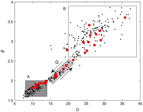
After this preliminary analysis, the values of D and E for each image are computed and reported in the D-E diagram. Fig. 4 shows the position of all the analyzed images in the diagram. Observe that the images are mainly organized in two regions, indicated by A (D ∼ [8,14], E ∼ [1.6,2]) and B (D ∼ [20,39], E ∼ [2.6,3.9]). The two regions are separated by a narrow zone depicted in gray (G).

Fig. 4.

Position of the images in the D-E diagram for the CGLE. The red circles refer to the value α = 0. We identify three regions: A, B, and G. For a fixed α and increasing β, the points move from region A(B) to region B(A) by crossing G (refer also to Movie S1). The arrows guide the eye for a better understanding of the points motion in the diagram.

It is worth noticing that points in region A are much more condensed with respect to region B. This is explained by the very low sensitivity of the GRQA measures, as mentioned before (Fig. 3). The role of the transition zone G becomes clear when looking at Movie S1, showing the dynamics of the points in the D-E diagram as functions of α and β. One can notice a systematic behavior: The points (i.e., the steady state solutions of the CGLE for a fixed pair (α,β)) are confined in one of the two regions (A or B), then move toward the other region by crossing the transition zone, and remain inside it. For example, consider the value α = 0. For increasing β, the points initially belong to A and remain in A until a critical value is reached; after this, the points cross G and jump in B for a new value . By increasing β, the scenario is observed again in the opposite direction: Starting from B, the points remain inside B until a critical value is reached, then they cross again G and jump in A after the value . The arrows in Fig. 4 indicate the directions along which the motion of the points for increasing β takes place.

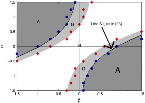
The behavior shown in Movie S1 and the regions with high and low sensitivity with respect to β suggest that it is possible to detect structural changes in the dynamics of the CGLE by looking at the region jumps. For each value of α, following the evolution of the points in the D-E diagram, we collect the values for which the transitions are observed and we report them in Fig. 5, where the blue circles correspond to the values of β for which the jumps G–A and A–G are observed, whereas the red diamonds correspond to the values of β for which the jumps G–B and B–G take place.

Fig. 5.

Identification of the transition curves in the parameter space. The line S₁ is the Eckhaus limit described in ref. 23. The red squares correspond to the values of β for which the transition B–G or G–B occurs. The blue circles are the values of β for which the transitions G–A and A–G occur. Notice that the symmetric line in the region β < 0 is also well reconstructed.

One can notice that the blue circles lie with good agreement on the Eckhaus stability limit (the line S₁ in paper (23). The region below the Eckhaus limit is mapped in the region A of the D-E diagram. Analogously, the unstable region of the parameter space is mapped to the region B, and the transition zone is mapped to the light gray zone G separating A and B. By looking at the values of β for which the jumps B–G and G–B happen, we identify with very good accuracy the transition region that was previously observed for some values of α and β by Huber et al. (21) and by Bohr et al. (25). They analyzed the onset of turbulence in the CGLE for finite domain size calling it transient turbulent behavior.

Reaction-diffusion systems

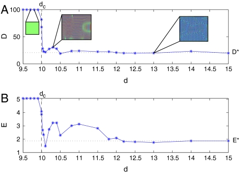
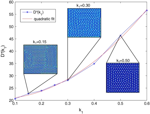
In this subsection the application of the proposed method to reaction-diffusion equations is discussed. Recently, the authors of the present paper have shown in (26) that determinism and entropy are suitable indicators for detecting different routes to Turing pattern formation in a Belousov–Zhabotinsky reaction performed in a water–oil microemulsion (27). Here we focus on one of the prototypical reaction-diffusion systems showing Turing bifurcations: the Schnakenberg model (28) (see Materials and Methods for mathematical details). Referring to Eq. 9 and according to ref. 29, we choose γ = 800, k₂ = 1, whereas k₁ varies in the range [0.1,0.6]. As expected, the Turing bifurcation can be easily detected by computing the recurrence indicators D and E. In fact, for diffusion coefficient smaller than the critical value d_c(k₁,k₂), the solution converges to a homogeneous state yielding the maximum feasible values of D and E. Fig. 6 shows the evolution of both D and E for k₁ = 0.1 and 9.8 < d < 15. Notice that near the critical value d_c ∼ 10 an abrupt change in both values of D and E indicates the occurrence of the bifurcation. Furthermore, for d > d_c, both indicators show some variations before reaching the saturation values D^∗(k₁ = 0.1) = 20.64, E^∗(k₁ = 0.1) = 1.868. This may be explained by the formation of transient patterns (Fig. 6, Insets) reported in ref. 29. Let us now collect the saturation values D^∗(k₁) and E^∗(k₁) for k₁∈[0.1,0.6]. Fig. 7 shows that D^∗(k₁) increases quadratically, whereas the same behavior is not observed for the entropy, whose regime value E^∗(k₁) ∼ 1.8 is independent of k₁. The behavior of both D^∗ and E^∗ can be explained by considering the Turing patterns: The increase of determinism may be related to the decrease of the spatial frequency of the patterns (Fig. 7, Insets). On the other side, entropy does not show important changes because the information does not vary significantly by reducing the spatial frequency.

Fig. 6.

Detection of the Turing bifurcation in the Schnakenberg model described by Eq. 9. The critical value d_c ∼ 10 is well identified by looking at the abrupt change of the indicators. For both determinism (A) and entropy (B), the saturation values D^∗, E^∗ are reached after a transient. The insets in (A) show the asymptotic patterns of the variable u: For d < d_c u is constant, for d ≳ d_c a spatial transient is observed (as reported in ref. 29), and the fully developed Turing pattern is observed for d > 12.

Fig. 7.

Plot of the saturation values D^∗(k₁) for k₁∈[0.1,0.6]. The curve is well fitted by a quadratic polynomial: the increase of the determinism D^∗ accounts for changes in the spatial distribution of the spotted patterns. By looking at the insets, one can notice decreasing spatial frequency of the spots for increasing values of k₁.

Conclusions

Reconsidering the experiment proposed at the beginning of the paper, we recognize that the pair of images (a),(b) falls in region A of Fig. 1, and the pair (e),(f) falls in region B, whereas the pair (c),(d) falls in region G. Then, with reference to Fig. 5, we can conclude that (a),(b) come from stable spiral wave solutions of the CGLE and (e),(f) come from unstable spiral wave solutions. Notice that, despite the different visual aspect, (a) and (b) refer to the same dynamical structure. This conclusion holds also for (e) and (f) but with different levels of determinism and entropy. Following the analysis performed in the paper, this indicates that the system underwent a transition by changing the parameter β. Moreover, the transition giving rise to images (c) and (d), takes place according to a path that is clearly visualized in Movie S1. The transition from (a),(b) to (e),(f), which has been clearly detected through the D-E diagram analysis, is not easily detectable by a visual inspection [e.g., notice that image (b) appears visually more different from (a) than from (d)]. It is worthwhile to remark that using different classical methods for measuring image complexity (like, for example, pixel-based entropy (30) fails to discriminate the different pattern structures in Fig. 1 (A)–(F) (15).

Summarizing, we have shown that the generalized recurrence quantification indicators are suitable for characterizing the spatial patterns of the complex Ginzburg–Landau equation. Specifically, following the evolution of the image positions in the D-E diagram, we were able to identify, for each value of α, a set of threshold values of β for which a region jump takes place. By collecting these values, it was possible to reconstruct, with good agreement, the Eckhaus limit of convective instability of spiral waves in the (α,β) plane. A transition zone of transient turbulence was reproduced extending the preceding results.

Regarding reaction-diffusion systems, we have considered the Turing patterns formed by the Schnakenberg model. As in the CGLE case, the quantification of spatial recurrences allowed for the detection of the different regimes observed in the pattern formation. In particular, the determinism was found to increase quadratically with the parameter k₁ of Eq. 9. Moreover, the transition from homogeneous to fully formed patterned states was easily detected.

The two examples addressed may be considered as prototypes for covering a wide range of phenomena. Furthermore, the technique proposed can be usefully applied either for detecting structural changes in unknown systems or for uncovering bifurcations in dynamical spatio-temporal systems, whose complexity prevents the application of classical bifurcation analysis (8, 31).

Indeed, there are several application areas where the proposed approach could help to understand the dynamical features of biological and physical phenomena from sporadic spatial data, such as spatial ecology (32), plankton turbulent patterns (33), physiology of tissues (2), and functional MRI (34). Further applications of the proposed method to these phenomena are the subject of ongoing work.

Materials and Methods

Complex Ginzburg-Landau Equation.

In the following only basic information is provided (for an exhaustive treatment of the CGLE the reader is referred to ref. 18). The CGLE reads

[3]

where and . The first term of the right hand side is related to the linear instability mechanism leading to oscillation. The second term accounts for diffusion and dispersion, whereas the cubic term insures, for β > 0, the saturation of the linear instability and is involved in the renormalization of the oscillation frequency. When α = 0 and β → ∞ one has the real Ginzburg–Landau Equation, which possesses a Lyapunov functional and exhibits relaxational dynamics (35). For α → ∞ and β = 0 one recovers the nonlinear Schrödinger equation. In two dimensions, the solutions of the CGLE are families of plane waves A = a_k exp ı(kx + ω_kt) with and ω_k = 1/β - (α + 1/β)k², where k is the wave number.

We have integrated the equation using a pseudospectral code (36), in a square domain of L = 512 points with periodic boundary conditions^†.

Generalized Recurrence Plots.

The recurrence plot (RP) (37) is essentially a two-dimensional binary diagram indicating the recurrences that occur in an m-dimensional phase space within a fixed threshold ϵ at different times i, j. For time series the RP is easily expressed as a two-dimensional square matrix with ones and zeros representing the occurrences (ones) or not (zeros) of states and of the system: , where , i,j = 1,…,N, N is the number of the measured states , Θ(·) is the step function, and ||·|| is a norm. In the graphical representation, each nonzero entry of R_i,j is marked by a black dot in the position (i,j). Because any state is recurrent with itself, the RP matrix fulfills R_i,i = 1 and hence contains the diagonal line of identity.

An RP is characterized by typical patterns, whose structure is helpful for understanding the underlying dynamics of the system investigated. A homogeneous distribution of points is usually associated with stationary stochastic processes; e.g., Gaussian or uniform white noise. Periodic structures, like long diagonal lines parallel to the line of identity indicate periodic behaviors, whereas drifts in the structure of the recurrences are often due to a slow variation of some parameter of the system and white areas or bands indicate nonstationarity and abrupt changes in the dynamics. For an extensive discussion of RPs and recurrence quantification analysis (RQA) measures the reader may refer to ref. 13. Recurrence plots may be exploited for the analysis of systems showing complex patterns in time and space. In ref. 14 the GRP for a d-dimensional data-set as the 2d-dimensional RP is defined by

[4]

where is the d-dimensional coordinate vector and is the associated phase-space vector. This GRP accounts for recurrences between the d-dimensional state vectors. The line of identity is replaced by a linear manifold of dimension d for which , .

The discretized solution of the two-dimensional CGLE at a fixed time can be represented by images (one for ℜ{A} and one for ℑ{A}); in this case the state or ℑ{A(x_i1,y_i2)} and the GRP reads as follows: R_i1,i2,j1,j2 = Θ(ϵ - ||x_i1,i2 - x_j1,j2||), i_k, , where each black dot represents a spatial recurrence between two pixels, and every pixel is identified by its coordinates (i₁,i₂), being i₁ and i₂ the row and the column index respectively. In this case, the recurrence plot is a four-dimensional RP and contains a two-dimensional identity plane, defined by setting i₁ = j₁ and i₂ = j₂.

Because the GRP of an image is four-dimensional, its visual inspection is possible only by projections in three or two dimensions. Although this is possible, relevant information is hard to extract, and one must cope with the fact that GRPs lose their visual appeal. Despite this drawback, RQA can still be performed because the structures described before can be easily extracted, and in the following we describe how to generalize the structures formed by the recurrences. A line structure of length l is composed by l consecutive recurrent points, according to the following formulation:

[5]

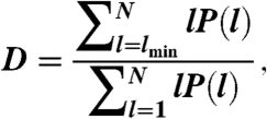
On the basis of the above definition, we build the histogram P(l) of the line lengths and define the GRQA measures as in the one dimensional case. In particular, we focus on recurrence rate (R), determinism (D) and entropy (E), defined as

[6]

[7]

[8]

where l_min is the minimum length considered for the diagonal structures.

The recurrence rate R is a density measure of the RP, accounting for the fraction of recurrent points in the spatial domain with respect to the total number of possible recurrences. Determinism (D) is a measure of the predictability of the system; in fact, it is the fraction of recurrent points forming diagonal structures in the RP with respect to all the recurrences. The entropy (E) is a complexity measure of the distribution of the diagonal lines in the GRP because it refers to the Shannon entropy with respect to the probability to find a structure of exactly length l.

The computation of the measures based on the diagonal lines and their distribution provides valuable information about the structure of the RP and the underlying structure of the solution under investigation. In particular, the determinism is the measure of the global pattern recurrence in the image: A value of determinism > 60–70% indicates that the image has strong recurrent components. In this sense, the measure fits the need to describe globally the patterns showed by the image. On the other side, the entropy provides a measure of the complexity of the GRP with respect to the diagonal structures: A low entropy indicates a poor organization of the line structures and is related to the small scale patterns.

Schnakenberg System.

The Schnakenberg system describes a simple chemical reaction with limit cycle behavior (28). It has been widely used for investigating Turing instabilities in biological and ecological systems (2). The dimensionless system of equations reads

[9]

where u(x,y,t), and x, y are the spatial variables; γ is proportional to the spatial domain size and represents the relative strength of the reaction terms, k₁ and k₂ depend on the reaction rates and d is the ratio of the diffusion coefficients of the two reactants. The critical diffusion coefficient d_c is a function of the parameters k₁ and k₂. For further details, the reader is referred to ref. 2, page 78.

The system has been integrated in a square domain of L = 250 points using a finite element method by means of Comsol Multiphysics software.

References

- 1.Epstein IR, Pojman J. An Introduction to Nonlinear Chemical Dynamics: Oscillations, Waves, Patterns, and Chaos. London: Oxford University Press; 1998. [Google Scholar]
- 2.Murray J. Mathematical Biology. 3rd Ed. Berlin: Springer; 2004. [Google Scholar]
- 3.Cross M, Greenside H. Pattern Formation and Dynamics in Nonequilibrium Systems. Cambridge, UK: Cambridge University Press; 2009. [Google Scholar]
- 4.Rutherford A, Aronson DG, Swinney HL. Patterns and Dynamics in Reactive Media (The IMA Volumes in Mathematics and its Applications) Vol 37. Berlin: Springer; 1991. [Google Scholar]
- 5.Janiaud B, et al. The Eckhaus instability for traveling waves. Physica D. 1992;55:269–286. [Google Scholar]
- 6.Cross M, Hohenberg PC. Pattern formation outside of equilibrium. Rev Mod Phys. 1993;65:852. [Google Scholar]
- 7.Grindrod P. Patterns and Waves: Theory and Applications of Reaction-Diffusion Equations. Oxford: Claredon Press; 1991. [Google Scholar]
- 8.Mei Z. Numerical Bifurcation Analysis for Reaction-Diffusion Equations. Berlin: Springer; 2000. [Google Scholar]
- 9.Banks H, Kunish K. Estimation Techniques for Distributed Parameter Systems. Basel: Birkhauser; 1989. [Google Scholar]
- 10.Vanag V, Epstein IR. Segmented spiral waves in a reaction-diffusion system. Proc Natl Acad Sci USA. 2003;100:14635–14638. doi: 10.1073/pnas.2534816100. [DOI] [PMC free article] [PubMed] [Google Scholar]
- 11.Guo L, Billings S. State-space reconstruction and spatio-temporal prediction of lattice dynamical systems. IEEE T Automat Contr. 2007;52(4):622–632. [Google Scholar]
- 12.Marcos-Nikolaus P, Martin-González JM, Solé RV. Spatial forecasting: Detecting determinism from single snapshots. Int J Bifurcat Chaos. 2002;12(2):369–376. [Google Scholar]
- 13.Marwan N, Romano M, Thiel M, Kurths J. Recurrence plots for the analysis of complex systems. Phys Rep. 2007;438:237–329. [Google Scholar]
- 14.Marwan N, Kurths J, Saparin P. Generalised recurrence plots analysis for spatial data. Phys Lett A. 2007;360:545–551. [Google Scholar]
- 15.Facchini A, Mocenni C, Vicino A. Generalized recurrence plots for the analysis of images from spatially distributed systems. Physica D. 2009;238:162–169. [Google Scholar]
- 16.Trulla LL, Giuliani A, Zbilut JP, Webber CL. Recurrence quantification analysis of the logistic equation with transients. Phys Lett A. 1996;223:255–260. [Google Scholar]
- 17.Huber G. Boston University; 1993. The onset of vortex turbulence. PhD thesis. [Google Scholar]
- 18.Aranson I, Kramer L. The world of the complex Ginzburg–Landau equation. Rev Mod Phys. 2002;74:99. [Google Scholar]
- 19.Sherratt J, Smith M, Rademacher J. Locating the transition from periodic oscillations to spatiotemporal chaos in the wake of invasion. Proc Natl Acad Sci USA. 2009;106:10890–10895. doi: 10.1073/pnas.0900161106. [DOI] [PMC free article] [PubMed] [Google Scholar]
- 20.Huber G. Vortex Solids and Vortex Liquids in a Complex Ginzburg–Landau System. In Spatio-Temporal Patterns in Nonequilibrium Complex Systems. In: Cladis PE, Palffy-Muhoray P, editors. Reading, MA: Addison–Wesley; 1995. [Google Scholar]
- 21.Huber G, Alstrom P, Bohr T. Nucleation and transients at the onset of vortex turbulence. Phys Rev Lett. 1992;69:2380. doi: 10.1103/PhysRevLett.69.2380. [DOI] [PubMed] [Google Scholar]
- 22.Brito C, Aranson IS, Chaté H. Vortex glass and vortex liquid in oscillatory media. Phys Rev Lett. 2003;90:068301. doi: 10.1103/PhysRevLett.90.068301. [DOI] [PubMed] [Google Scholar]
- 23.Chaté H, Manneville P. Phase diagram of the two-dimensional complex Ginzburg–Landau equation. Physica A. 1996;224:348–368. [Google Scholar]
- 24.Manneville P, Chaté H. Phase turbulence in the two-dimensional complex Ginzburg–Landau equation. Physica D. 1996;96:30–46. [Google Scholar]
- 25.Bohr T, Pedersen A, Jensen M. Transition to turbulence in a discrete Ginzburg–Landau model. Phys Rev A. 1990;42:3626. doi: 10.1103/physreva.42.3626. [DOI] [PubMed] [Google Scholar]
- 26.Facchini A, Rossi F, Mocenni C. Spatial recurrence strategies reveal different routes to Turing pattern formation in chemical systems. Phys Lett A. 2009;373(46):4266–4272. [Google Scholar]
- 27.Vanag VK, Epstein IR. Segmented spiral waves in a reaction-diffusion system. Proc Natl Acad Sci USA. 2003;100(25):14635–14638. doi: 10.1073/pnas.2534816100. [DOI] [PMC free article] [PubMed] [Google Scholar]
- 28.Schnakenberg J. Simple chemical reaction systems with limit cycle behavior. J Theor Biol. 1979;81:389–400. doi: 10.1016/0022-5193(79)90042-0. [DOI] [PubMed] [Google Scholar]
- 29.Madzvamuse A, Wathen AJ, Maini PK. A moving grid finite element method for the simulation of pattern generation by Turing models on growing domains. J Comput Phys. 2003;190:478–500. [Google Scholar]
- 30.Gonzalez R, Woods R, Eddins S. Digital Image Processing Using MATLAB. Englewood Cliffs, NJ: Prentice Hall; 2003. [Google Scholar]
- 31.Hirsch MW, Smale S. Differential Equations, Dynamical Systems, and Linear Algebra. London: Academic; 1974. [Google Scholar]
- 32.Allegretto W, Mocenni C, Vicino A. Periodic solutions in modelling lagoon ecological interactions. J Math Biol. 2005;51:367–388. doi: 10.1007/s00285-005-0325-7. [DOI] [PubMed] [Google Scholar]
- 33.Abraham E. The generation of plankton patchiness by turbulent stirring. Nature. 1998;391:577–580. [Google Scholar]
- 34.Huettel SA, Song AW, McCarthy G. Functional Magnetic Resonance Imaging. Sunderland, MA: Sinauer; 2004. [Google Scholar]
- 35.Graham R. Hydrodynamic fluctuations near the convection instability. Phys Rev A. 1974;10:1762. doi: 10.1103/physreva.45.4198. [DOI] [PubMed] [Google Scholar]
- 36.Cox S, Matthews P. Exponential time differencing for stiff systems. J Comput Phys. 2002;176:430–455. [Google Scholar]
- 37.Eckmann JP, Kamphorst SO, Ruelle D. Recurrence plot of dynamical systems. Europhys Lett. 1987;5:973–977. [Google Scholar]
Associated Data
This section collects any data citations, data availability statements, or supplementary materials included in this article.