The Copenhagen Accord for limiting global warming: Criteria, constraints, and available avenues

Abstract

At last, all the major emitters of greenhouse gases (GHGs) have agreed under the Copenhagen Accord that global average temperature increase should be kept below 2 °C. This study develops the criteria for limiting the warming below 2 °C, identifies the constraints imposed on policy makers, and explores available mitigation avenues. One important criterion is that the radiant energy added by human activities should not exceed 2.5 (range: 1.7–4) watts per square meter (Wm⁻²) of the Earth's surface. The blanket of man-made GHGs has already added 3 (range: 2.6–3.5) Wm⁻². Even if GHG emissions peak in 2015, the radiant energy barrier will be exceeded by 100%, requiring simultaneous pursuit of three avenues: (i) reduce the rate of thickening of the blanket by stabilizing CO₂ concentration below 441 ppm during this century (a massive decarbonization of the energy sector is necessary to accomplish this Herculean task), (ii) ensure that air pollution laws that reduce the masking effect of cooling aerosols be made radiant energy-neutral by reductions in black carbon and ozone, and (iii) thin the blanket by reducing emissions of short-lived GHGs. Methane and hydrofluorocarbons emerge as the prime targets. These actions, even if we are restricted to available technologies for avenues ii and iii, can reduce the probability of exceeding the 2 °C barrier before 2050 to less than 10%, and before 2100 to less than 50%. With such actions, the four decades we have until 2050 should be exploited to develop and scale-up revolutionary technologies to restrict the warming to less than 1.5 °C.

The unsuccessful Kyoto Protocol's first commitment period comes to an end in 2012. The 15th Conference of the Parties (COP-15) of the United Nations Framework Convention on Climate Change met December 7–19, 2009, in Copenhagen to arrive at an international agreement for mitigating climate change. An agreement could not be reached; instead, the COP-15 arrived at the so-called “Copenhagen Accord” (CHA). Of the 193 nations that attended, including the leaders of major developed and developing nations, all but a few nations (Bolivia, Cuba, Nicaragua, Sudan, and Venezuela) supported the accord. The most significant part of the succinct three-page 12-paragraph CHA (1) is the following: “We underline that climate change is one of the greatest challenges of our time” in its opening paragraph, followed by the second paragraph, which begins with “We agree that deep cuts in global emissions are required according to science, and as documented by the IPCC Fourth Assessment Report with a view to reduce global emissions so as to hold the increase in global temperature below 2 degrees Celsius, and take action to meet this objective consistent with science and on the basis of equity.” Targets for greenhouse gas (GHG) emission reductions as required by Appendix 1 of the CHA have already been provided by over 100 countries, including most if not all of the major emitters. The initial response to the CHA was one of disappointment (2), particularly because it did not include binding targets for reductions in CO₂ emissions. As such, the CHA is considered to be just a political document (2).

The present article, on the other hand, argues that an agreement to limit the warming below 2 °C is significantly more formidable than requiring 50–80% reductions in CO₂ emissions before 2100. In what follows, we develop the criteria imposed by the 2 °C barrier, the constraints faced by policy makers, and available avenues for limiting the warming (summary provided in Box 1). The overarching principle that emerges from the present analyses (Box 2) is that we have to evolve from the CO₂-based approach of climate management pioneered by several studies (3–8) into one that integrates the management of the carbon budget with the radiant (IR and solar) energy budget of the planet (3–8).

Box 1. Meeting the Challenges of the CHA.

Criteria.

• The 2 °C warming limit places a barrier on the radiant energy added by human activities at 2.5 (range: 1.7–4) Wm⁻². The corresponding limit on CO_2,E is 441 (range: 380–580) ppm.

• CO₂ concentration has to be stabilized below 441 ppm before 2100.

• Air pollution laws that reduce the masking effect of cooling aerosols must enforce offsetting reductions in BC and ozone to remain radiant energy-neutral.

Constraints.

• The radiant energy barrier of 2.5 Wm⁻² has already been exceeded by 20%.

• The inadvertent unmasking of the warming by air pollution laws places a severe constraint on mitigation.

Avenues.

Manage the budget of both carbon and radiant energy.

• Decrease the rate of thickening of the blanket of GHGs: Stabilize CO₂ concentration below 441 ppm.

• Offset the addition of radiant energy resulting from the reduction of aerosol cooling: Reduce BC and ozone concentrations.

• Thin the GHG blanket: Reduce emissions of methane and HFCs. By 2050, have scalable technologies ready to extract BC, methane, and CO₂ from the atmosphere.

Box 2. CO₂ and Non-CO₂ GHGs, BC, and Aerosol Masking.

CO₂ (1.65 Wm⁻²) and the non-CO₂ GHGs (1.35 Wm⁻²) have added 3 (range: 2.6–3.5) Wm⁻² of radiant energy since preindustrial times. The non-CO₂ GHGs are methane (CH₄); nitrous oxide (N₂O); and halocarbons (HCs), which include CFCs, HCFCs, HFCs; and ozone in the troposphere. The 3-Wm⁻² energy should have led to a warming of 2.4 °C (14). The observed warming trend (as of 2005) is only about 0.75 °C (15), or 30% of the expected warming. Observations of trends in ocean heat capacity (16) as well as coupled ocean–atmosphere models suggest that about 20% (0.5 °C warming) is still stored in the oceans (17). The rest of the 50% involves aerosols or particles added by air pollution. BC aerosols in soot absorb solar radiation and add 0.5 (inner white circle) to 0.9 Wm⁻². SON_Mix of particles from fossil fuel and biomass combustion act like mirrors and reflect solar radiation back to space (−2.1 Wm⁻²; the transparent blue-shaded circle). The resulting dimming effect at the surface has been observed in land stations around the world (18, 19). The net aerosol masking effect (−2.1 + 0.9 = −1.2 Wm⁻²), along with the 0.2-Wm⁻² cooling by land surface changes, accounts for the missing 50% of the warming by GHGs. There is at least a 3-fold uncertainty in current estimates of the aerosol masking effect (the inner and outer circle of the net forcing in the figure), which has significant implications for 21st century warming as explained later.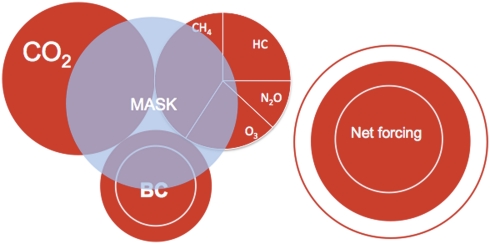

Box 2 Figure. Area of each red-shaded circle is proportional to the energy addition from preindustrial time to 2005. All the numbers, except the BC number, are taken from the article by Forster et al. (13). Radiant energy addition by methane includes the production of stratospheric water vapor by methane oxidation. Methane is also responsible for about 50% of the energy addition by ozone. Similar pie charts for years 2050 are shown in Fig. S2.

The 2 °C CHA barrier is based on recommendations by numerous scientific studies (3–8), which suggest that global warming in excess of 2 °C can trigger several climate-tipping elements and lead to unmanageable changes. It is also likely that the 2 °C barrier will be revised to lower values as regional consequences are better understood (5–8), a possibility that is also acknowledged by the CHA in its concluding paragraph.

Criteria for the 2 °C Barrier

Developing the criteria for the 2 °C limit is elegantly simple. A synthesis of empirical and 3D climate model studies (9) leads to the conclusion that the climate system should warm by 0.8 °C (range: 0.5–1.2 °C) per watts per square meter (Wm⁻²) of the Earth's surface increase in the input of radiant (IR and solar) energy. Basically, the radiant energy added by human activities cannot exceed 2.5 (range: 1.7–4) Wm⁻². The 2 °C temperature barrier translates into a 2.5-Wm⁻² barrier for the energy addition and equals 1,280 terawatts (10¹² W) of energy when summed over the globe. For comparison, the global energy consumption by human activities is 15 terawatts (10). The addition of radiant energy to the climate system is also referred to as radiative forcing. The energy budget criteria can be converted into a metric frequently used by policy makers, the equivalent CO₂ (CO_2,E) concentration that will give rise to the 2.5-Wm⁻² energy addition. The analytical equation consistent with CO₂ spectroscopy is given by the equation H′ = H₀ ln [(CO_2,E)/CO₂,_Ref] (11), where the constant H₀ = 5.5 Wm⁻² (12) and CO₂,_Ref is the preindustrial era CO₂ reference concentration, taken to be 280 ppm. Substitution of H′ = 2.5 (range: 1.7–4) Wm⁻² in this equation yields the equivalent criteria CO_2,E = 441 (range: 380–580) ppm.

Policy Makers’ Dilemma

The 2.5-Wm⁻² barrier poses a huge dilemma for policy makers because the blanket of man-made GHGs that surrounds the planet as of 2005 has already trapped 3 (range: 2.6–3.5) Wm⁻² (13) (Box 2). The most severe constraint faced by policy makers is that the radiant energy barrier of 2.5 Wm⁻² has already been exceeded by 20%.

Challenges for Policy Makers

The planet is very likely to experience warming in excess of 2 °C if policy makers stringently enforce existing air pollution laws and remove reflecting aerosols without concomitant actions for thinning the GHG blanket (14, 20). Reducing emission of long-lived GHGs such as CO₂ will not thin the blanket this century because of the century to 1,000 years lifetime of CO₂ molecules in the air. Reductions in CO₂ emissions are essential to prevent further thickening of the blanket, however (21, 22). The other option is to keep polluting the air with reflecting particles (Box 2). However, the particles reduce air quality, have negative health effects, and produce “acid” rain (23). The particles can also suppress rainfall and lead to droughts, especially in the tropics (24, 25). A third option is to hope for the 10% or less probability (14) that climate is more resilient than projected by most climate models; that is, instead of warming by 0.8 °C per Wm⁻² of heat addition, it warms less than 0.5 °C per Wm⁻². Policy makers can hope for the best, but a prudent approach would be to plan for more probable outcomes.

Avenues for Managing the Watts

The model proposed here is a combination of the so-called “carbon budget” approach (4, 26, 27) and the radiant energy budget approach proposed in the present study. The carbon budget approach limits the cumulative CO₂ emissions from now until 2050 or 2100 to a prescribed amount. The radiant energy budget approach limits the net (GHGs + aerosols) watts added by human activities to 2.5 (range: 1.7–4) Wm⁻². There are three avenues for managing the watts added to the system.

The quantitative mitigation potentials of the three avenues and the probability of limiting the warming to 2 °C are illustrated with a model (40–42) (model description provided in Box 3).

Box 3. An Integrated Carbon and Radiant Energy Budget Climate Model.

The model links emissions of pollutants with their atmospheric concentrations and the change in the energy input. The emission model (40) is coupled with an energy balance climate model with a 300-m ocean mixed layer to simulate the temporal evolution of global mean surface temperature. Such models are well documented (41). The model accounts for historical variations in the energy input to the system attributable to natural factors, GHGs, and air pollutants (i.e., SO₂, NO + NO₂, CO, BC, organic carbon) (13). The natural factors include variations in energy input on interannual (13), 11-year solar cycle (13), and multidecadal (60 years) (42) scales. The model is calibrated by comparing it with the observed 20th century changes in CO₂ concentrations (Fig. 1A in this box), in temperature (Fig. 1B in this box), and in the heat content of the global ocean (Fig. 1C in this box). Without the natural factors, the model would be unable to simulate the temporal patterns, particularly the steep warming trend during the 1910s to 1940s followed by three decades of a weak cooling trend.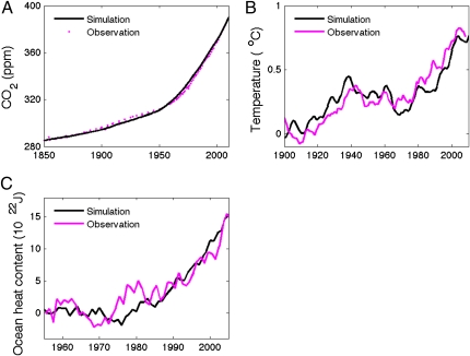

Box 3 Figure. Comparison of model simulation with observation is illustrated. (A) CO₂ concentration as simulated from a mixed-layer pulse response model (40). Data on CO₂ emission and observed atmospheric concentration are from the Carbon Dioxide Information Analysis Center. (B) Temperature increase as simulated from the energy balance model compared with Goddard Institute for Space Studies data (anomaly relative to 1900–1910). (C) OHC as simulated in the model, compared with observation by Levitus et al. (16) (anomaly relative to 1957–1967).

Avenue i: Decrease the Rate of Thickening of the GHG Blanket.

We must prevent the problem from getting much worse. As of 2005, fossil fuel burning and land use change since 1750 have added about 776 billion tons (Gt) of CO₂ (i.e., 99 ppm) to the atmosphere. The annual CO₂ emission was about 35 Gt CO₂ in 2005 (Fig. 1A) and has been growing at about 2–3% annually since then. Even if the emission peaks in 2015 and remains at that level until 2100, CO₂ concentration will exceed 550 ppm (3, 4) (SI Text and Fig. S1) and will add another 2 Wm⁻² by 2100. This will bring the preindustrial to 2100 energy added by GHGs to 5 Wm⁻² (from the 2005 value of 3 Wm⁻²), which is about 100% larger than the 2.5-Wm⁻² barrier. The criterion that emerges is that any mitigation strategy must start with drastic CO₂ emission reductions to stabilize CO₂ concentrations below 441 ppm during this century. The required reductions are in the range of 50% by 2050 and 80% before 2100 as recommended by the carbon budget approach outlined elsewhere (4, 26, 27) (Fig. 1A). The blanket will still get thicker, but CO₂ concentration will stabilize at less than 441 ppm during the 21st century (4, 26, 27) (Fig. 1B).

Fig. 1.

(A) Historical and projected CO₂ emissions. (B) Historical and projected CO₂ atmospheric concentration under the CO₂ emission in A. (C) CO_2,E concentration and corresponding radiant energy addition. The red line includes only GHGs; the blue and black lines account for GHGs, particles, and solar and land use change forcing. Beyond 2005, the red line assumes mitigation of CO₂ as shown in A, but non-CO₂ GHGs increase following the BAU model; the blue line is same as the red line, except it includes the aerosol cooling effect and its reduction from 2015 onward; and the black line is the FMA and is same as the blue line, except it includes mitigation of non-CO₂. (D) Energy balance model simulations of past and future temperatures (using the forcing in C; blue and black lines also account for variation in 60-year natural cycle). Pink and yellow backgrounds show zones beyond 2 °C and 1.5 °C.

Halving the CO₂ emissions by 2050 is a forbidding challenge requiring massive decarbonization of many anthropogenic activities. It requires a portfolio of actions in the energy, industrial, agricultural, and forestry sectors such as conservation and efficiency improvement to reduce the carbon intensity of energy use, aforestation, replacement of fossil fuels with renewables, carbon capture and storage, and numerous other steps (27, 28). In contrast, as discussed below, the actions listed under avenues ii and iii are achievable using existing technologies and stringent application of existing air pollution polices.

Avenue ii: Offset Warming from the Reduction of Aerosol Masking.

The major contributors to the reflecting aerosols are sulfates from SO₂ emission, nitrates from NO_x (NO + NO₂) emission, and organic aerosols from combustion of fossil and biomass fuels. Experimental results have shown that these aerosols occur as internal mixtures (29), whose chemical and radiative properties are quite different. Accordingly, this study refers to aerosols as sulfates-organics-nitrates mixtures (SON_Mix). Worldwide SO₂ emissions increased from about 10 million tons of sulfur per year (Mt S/yr) to a peak of 65–70 Mt S/yr in the early 1980s and have been declining since then to about 55 Mt S/yr as of 2000 (30). The resulting increases in visibility and solar radiation at the surface have been recorded in Europe and North America (31), accompanied by warming trends (32, 33). Projections call for about a 60% reduction in SO₂ emissions by 2050, with stricter enforcement of air pollution laws (34). Such a move can unmask much of the potential warming effect of anthropogenic GHGs.

Fortunately, there are two independent paths to accomplish this seemingly Herculean task. First, air pollutants also lead to black carbon (BC) aerosols that trap (absorb) solar radiation in the atmosphere and heat the blanket directly. BC, a major contributor to warming (35–37) (Box 2), has a very short lifetime of days to weeks. Reductions in BC emissions will immediately lead to a reduction in the energy input to the system. Second, air pollution also produces ozone, which is a strong GHG, in the lower atmosphere (38). Methane, NO_x, CO, and nonmethane volatile organics (NMVOCs) are the gases that produce ozone. NO_x contributes to production of near-surface ozone. Methane, CO, and NMVOCs lead to ozone production within the entire troposphere (13). Methane contributes about 50% of the ozone greenhouse effect (Box 2), CO and NMVOCs contribute another 35%, and the balance is contributed by NO_x (13, 39). In our model, the ozone reduction is caused by reductions in methane and CO. All these ozone precursors, except methane, fall under the category of air pollutants. The lifetime of ozone is about a month; hence, energy addition attributable to ozone will respond quickly to mitigation actions.

Avenue iii: Thin the Greenhouse Blanket.

Finally, we must reduce the 3 Wm⁻² that is already in the system. We can thin the blanket by reducing emissions of short-lived GHGs: methane and hydrofluorocarbons (HFCs). As noted under avenue ii above, reduction of methane emission will also reduce ozone. Methane reductions also pose huge challenges. About 33–45% of the annual CH₄ emission of 230–300 Mt is caused by livestock and the agriculture sector, 30% is caused by the energy sector, and 25% is caused by waste treatment and disposal (13, 27, 28). The required actions include reduced pipeline leakage in the gas sector, productivity improvements in livestock management and rice cultivation, and reduction of CH₄ emissions from landfills and coal extraction with subsequent recovery for energy purposes.

Mitigation Potentials of the Three Avenues

The basic assumption is that emissions of all the GHGs will continue to grow until 2015. CHA mitigation actions are assumed to go into full implementation in 2015. The mitigation avenues are guided by the following two objectives: to reduce the probability of a warming in excess of 2 °C before 2050 to less than 10%, and to reduce the probability of the warming exceeding 2 °C before 2100 to less than 50%. In what follows, we describe each avenue. The case that employs all three is referred to as the full-mitigation avenue (FMA).

The business as usual (BAU) scenario is that emission of CO₂ will peak at 2015 and remain at the 2015 level until 2100 and that the emissions of non-CO₂ GHGs will peak at 2030 (34). In addition, current air pollution laws for reducing SO₂ emissions in developed nations will be implemented worldwide, particularly in China and India. This assumption is justified on the basis that air pollution is a major source of concern in these countries (more so than the climate change concerns) and the so-called “Euro-standards” are being implemented in China and India (43). Clearly, the BAU scenario, even though it stabilizes emissions, violates all the criteria (Box 1). About 2.7 Wm⁻² will be added from 2005 to 2050 (Fig. 2, Left), such that the net (GHGs + aerosols) energy added from the preindustrial era to 2050 will exceed 4 Wm⁻².

Fig. 2.

Projected changes in energy input from 2005 to 2050 for two mitigation avenues. (Left) BAU. (Right) Mitigation of CO₂, SO₂, and all other non-CO₂ agents as described in text for the FMA.

The avenue for stabilizing CO₂ concentration is the carbon budget approach (4, 26, 27). The cumulative emission of CO₂ (both fossil fuel and land use change) from 2010 to 2050 is limited to 950 Gt of CO₂, and the cumulative emission from 2050 to 2100 is reduced to 425 Gt of CO₂. These emissions are within 15% of those articulated by the carbon budget approach to limit warming to 2 °C. CO₂ concentration will peak at about 430 ppm by 2050 (Fig. 1B). The radiant energy added by the increase of CO₂ from the preindustrial era to 2050 will be 2.3 Wm⁻². If human activities add no further watts to the system, such an action, by itself, would be sufficient to limit the warming to 2 °C. This is not likely to occur, however. With an increase in population from 6.5 to 9 billion during this century, we must allow for BAU increases in non-CO₂ GHGs that will add another 0.7 Wm⁻² (Fig. 2, Left). The warming attributable to just the GHGs can exceed 3 °C (Fig. 1D, red line), and we will be more dependent on the mirrors to mask this warming (Fig. 1D, difference between red and blue lines). Unfortunately, time may be running out for this option too. As projected (34), extension of current air pollution laws to the rest of the world can reduce SO₂ emissions by as much as 60% by 2050. The resulting reduction of the SON_Mix cooling can add another 0.65 Wm⁻² (Fig. 2, Left). Even with a drastic CO₂ reduction, the net (GHGs + aerosols) energy addition from 2005 to 2050 is about 2.2 Wm⁻² (Fig. 1C, blue line) and the warming can exceed 2 °C before 2050 (Fig. 1D, blue line).

The deduction above may seem inconsistent with recent studies (4, 26), but it is not. These earlier studies assume a 50% reduction in all GHG emissions and furthermore implicitly assume that the reduction of the aerosol cooling effect by SO₂ reductions will be mostly compensated for by increases in nitrate aerosols from NO_x pollution. The latter assumption of offsetting SO₂ pollution with NO_x pollution is not supported by recent studies (34, 43), which show that technologies exist to reduce SO₂ as well as NO_x emissions significantly during this century. The offsetting effect of NO_x pollution is also not supported by surface solar data (31–33), which reveals brightening in most of the developed nations during the past few decades in response to stringent enforcement of air pollution laws. Finally, building in such a Faustian bargain may not be desirable, given the damaging effects of NO_x on human health and agriculture (44). Thus, another severe constraint in our ability to limit the energy addition is the inadvertent reduction of the aerosol cooling effect.

We have to complement CO₂ and SO₂ reductions with reductions in other warming agents resulting from air pollution, which are BC and the pollutant gases that produce tropospheric ozone (3, 14, 22, 45). Estimates for solar energy addition to the atmosphere by BC as of 2005 range from 0.5–1 Wm⁻² (13, 35, 46). Studies that constrain BC effects by satellite and in situ observations yield 0.8–1 Wm⁻² (36, 46), and model studies that adopt a realistic mixing of BC with SON_Mix (35, 47) yield 0.5–0.8 Wm⁻². In addition, BC, when deposited on ice and snow, increases solar absorption and adds another 0.05–0.1 Wm⁻² (13) to the surface. This direct warming is also estimated to be a major factor in the observed warming of the Arctic (37, 48) and the Himalayan-Tibetan glacier region (49, 50). We adopt 0.9 Wm⁻² for the BC energy addition from the preindustrial era (before 1750) to 2005, which translates to 0.6 Wm⁻² for the period from 1900 to 2005. In a later section that explores uncertainties in aerosol effect, we allow for a 50% uncertainty in the BC energy addition.

The third criterion that emerges is that air pollution regulations that reduce the masking effect of cooling aerosols must also include reductions in emissions of BC and ozone-producing gases to remain watt-neutral.

We adopt the recommendation of the studies by the International Institute for Applied Systems Analysis (IIASA) (34) and the Royal Society (43) that maximum feasible reductions of air pollution regulations can result in reductions of 50% in CO emissions, 30% in methane emissions by 2030, and 50% in BC emissions by 2050. Furthermore, extension of the Montreal Protocol to include HFCs and hydrochlorofluorocarbons (HCFCs) will reduce the total halocarbon [chlorofluorocarbons (CFCs) + HCFCs + HFCs] forcing by 30% from its 2005 value of 0.35 Wm⁻² (51). Without such a step, HFCs alone can add another 0.4 Wm⁻² by 2050 (51). Technologies are available to achieve these reductions (21, 34). When combined with a 50% CO₂ reduction by 2050, non-CO₂ reductions with current technologies can limit the post-2005 net (GHGs + aerosols) energy addition to about 0.7 Wm⁻² (Fig. 2, Right). The simulated warming for the FMA careens slightly below the 2 °C threshold (Fig. 1D, black line).

Regulatory policies and forums exist to reduce non-CO₂ warming agents. The Montreal Protocol with modifications for HFC regulations (21) can be an effective tool for reducing watts attributable to HFCs (21, 51). National policies exist to limit CO and other ozone-producing gases (34). These can be extended to enforce methane reductions, because methane contributes more than 50% to the production of ozone (9). BC is already implicitly included in air pollution regulations that set standards for particle emissions (35, 45, 52). These regulations have to be made more explicit. Such fast-track actions will be a major incentive for policy makers and political leaders (21). The impact of their actions on human health and environment should be visible during their tenure.

Need for Verification of the Approach

We need to start demonstration projects and conduct field experiments to evaluate the true impact of the various air pollution mitigation options outlined here. Current estimates, including the ones shown here, are model-based values. Let us take the case of BC. Sources that emit BC also emit organic carbon. Some of the organics absorb solar radiation, also referred to as brown carbon, whereas others reflect solar radiation (53). The mix of BC and organics can also modify clouds (54–56), in turn, amplifying the radiant energy input by BC. Thus far, it is clear that BC warming effects dominate over the organics for fossil fuels and that BC mitigation efforts must start with diesel fuel (57). Fortunately, regenerative filters for diesel vehicles that reduce BC emissions by up to 99% (52) are available in the market and are in use. The situation is different for biomass cooking, which emits more organics and also emits methane and CO, both of which produce ozone and thus amplify the warming effect of BC. We need scientifically monitored intervention field studies. One such study is Project Surya (58), which was developed for rural India to evaluate the global warming role of BC from biomass cooking.

Coping with Uncertainties in Climate Science

There is about a 50% probability that climate is more sensitive than the central value used here (9, 59). Probability density functions (pdfs) for climate sensitivity have been estimated by climate models (9, 59). The corresponding pdfs for the FMA are shown in Fig. 3. The FMA reduces the probability of warming in excess of 2 °C before 2050 to less than 10%. However, the 2100 pdf reveals that even the FMA has only a 50% probability of limiting warming below 2 °C. Another source of surprises in the projected outcomes is that the large uncertainties in the aerosol cooling and the BC warming may go the wrong way to accelerate the warming. For example, it is not inconceivable that the BC forcing is smaller (or larger) by 50% and that the negative value of SON_Mix masking is also smaller (or larger) by 50%, such that the sum of the BC energy addition and the SON_Mix masking can be as low as −1.8 Wm⁻² (60) (or as large as −0.5 Wm⁻²). If it is −0.5 Wm⁻², the net energy added to the system as of 2005 is already at 2.5 Wm⁻² (3 Wm⁻² from GHGs and −0.5 Wm⁻² from aerosols). However, the climate sensitivity has to be smaller by a factor of 2 to explain the 0.76 °C observed warming (also refer to ref. 61). If, on the other hand, it is −1.8 Wm⁻², unmasking during the coming decades can lead to a large addition of energy and warming can exceed 2 °C before 2100 (Fig. 4A, black line). Which of the three cases is more realistic? Models with aerosol effect between −1.4 Wm⁻² and −0.5 Wm⁻² agree better with temperature trends (Fig. 4A), whereas models with aerosol cooling effect in the range of −1.8 to −1.4 Wm⁻² simulate better the observed trend of energy added to the oceans (Fig. 4B), which is discussed next. Uncertainty in aerosol forcing has a profound effect on the projected 21st century temperature changes (Fig. 4A). However, these and other uncertainties do not obviate the fact that man-made GHGs have already added 3 Wm⁻² of radiant energy and, if unchecked, can add another 3 Wm⁻² during this century. The 6 Wm⁻² is equivalent to a 2.5% increase in the brightness of the sun or the estimated energy (e.g., 6) it took to switch the planet from its glaciated stage about 20,000 years ago to its current interglacial period.

Fig. 3.

Pdfs of simulated future temperature (in the years 2050 and 2100 for the FMA; same forcing as black lines in Fig. 1C). The uncertainty is from climate sensitivity uncertainty, and a confidence level >90% is shown in shade because of poor understanding of the tail of the distribution toward high warming rates. The distribution in the shaded region should be treated as unreliable.

Fig. 4.

(A) Simulated temperature increases under three aerosol forcing cases (−0.5 Wm⁻², −1.4 Wm⁻², and −1.8 Wm⁻²). The aerosol forcing is the sum of the energy addition by BC and the masking by SON_Mix. The uncertainty range shown here is consistent with published summaries (13). Climate sensitivity in each run is adjusted to mimic the 20th century warming trend and/or the ocean heating. Observation is from the Goddard Institute for Space Studies dataset. (B) Ocean heating, which is the time rate of change of ocean heat content. Observed values for 1960–2000 are from Levitus et al. (16), and observed values for 2003–2008 are from Schuckmann et al. (62).

A Powerful Diagnostic Tool

A fundamental quantity that can give us critical insights is the energy added to the ocean (Fig. 4B), which is the rate of change of ocean heat content (OHC) with time. Since the 1960s, OHC has been measured with sufficient accuracy (16, 62). A recent study of observed temperature variations in the ocean through 2,000 m depths (62) shows that the 2003–2008 period witnessed a large energy addition of about 0.77 Wm⁻², consistent with present simulations (Fig. 4B). The most important inference from Fig. 4B is that irrespective of the magnitude of the aerosol masking, the OHC response to mitigation actions shows a reversal in the positive trend of ocean energy addition to negative within two decades after the mitigation actions begin, well before 2050 and well before the temperature trends show a reversal (compare Fig. 4A with Fig. 4B). If this finding with the simple climate model is verified by 3D atmosphere–ocean climate models, the time rate of change of OHC would prove to be a powerful diagnostic for evaluating the success of mitigation actions.

Available Avenues for Coping with Rapid and/or Abrupt Warming

Let us now consider the less than 50% probability that warming exceeds 2 °C before 2100 (Fig. 3, blue line). Such abruptly large warming can trigger natural feedbacks such as methane ventilation from permafrost and the Arctic Shelf (63, 64) or a more rapid retreat of Arctic sea ice (65) and Alpine glaciers (66) and snow packs. Available avenues for such extreme events can be classified under two categories: passive and invasive geoengineering (67, 68).

Passive geoengineering basically involves thinning the blanket by capturing CO₂ [e.g., using bio-char to convert agriculture waste to charcoal (69)], methane, and BC directly from the air. Using a time frame of 50 years, we estimate that capturing 1 ton of BC or 20 tons of methane at the source will have the same effect on the watts as capturing 3,000 tons of CO₂ (also refer to ref. 57). Although there are currently many efforts at capturing carbon in CO₂ (20), we need to initiate research efforts to capture BC and the non-CO₂ GHGs, particularly methane and CO. The main advantage of non-CO₂ warmers is that the weight of the material to be captured is on the order of millions of tons and not billions of tons as in the case of CO₂. If enough CO₂, methane, and BC can be removed from the air, beginning in 2050, to reduce the energy addition by 0.1 Wm⁻² each, the probability of exceeding 2 °C by 2100 will be smaller than 15% compared with the 50% probability for the FMA case.

Invasive geoengineering involves many proposed solutions, but the ones that have received the most scrutiny are to add more reflecting particles in the stratosphere or to nucleate more cloud drops (67, 68). Even these measures are proposed only under extreme situations such as the planet witnessing large and abrupt climate changes (67, 68). Both of these options have unintended consequences (25) such as slowing down the global water cycle (24) or altering regional solar heating gradients, which can, in turn, change regional wind patterns in unpredictable ways (19). The results shown here clearly suggest that we have to start examining these options, including scrutinizing the ethical and moral dimensions (70). However, a broad-based mitigation strategy that includes both GHGs and air pollutants has the best chance for avoiding such unchartered avenues.

Fortunately, there is a great success story and a field-tested regulatory model in the case of non-CO₂ climate warmers. The enormous greenhouse effect of CFC-11 and CFC-12 was identified in the 1970s (71), which revealed that the radiant energy addition per molecule of CFC-11 or CFC-12 was more than 10,000 times that of the CO₂ molecule. CFCs were regulated by the Montreal Protocol in 1987 because of their negative effects on stratospheric ozone. Had CFC-11 and CFC-12 not been regulated, their greenhouse effects would have added 0.6–1.6 Wm⁻² of radiant energy by now (72) and could have exceeded the CO₂ effect during this century. We just have to repeat this successful model of avoiding dangerous climate changes.

References

- 1.United Nations Framework Convention on Climate Change Copenhagen Accord. 2009. [Accessed April 14, 2010]. Available at http://unfccc.int/resource/docs/2009/cop15/eng/l07.pdf.
- 2.Stavins R. What hath Copenhagen wrought? A preliminary assessment of the Copenhagen Accord. 2009. [Accessed April 14, 2010]. Available at http://belfercenter.ksg.harvard.edu/analysis/stavins/?p=464.
- 3.Schellnhuber HJ. Global warming: Stop worry-ing, start panicking? Proc Natl Acad Sci USA. 2008;105:14239–14240. doi: 10.1073/pnas.0807331105. [DOI] [PMC free article] [PubMed] [Google Scholar]
- 4.Meinshausen M, et al. Greenhouse-gas emission targets for limiting global warming to 2 degrees C. Nature. 2009;458:1158–1162. doi: 10.1038/nature08017. [DOI] [PubMed] [Google Scholar]
- 5.Kriegler E, Hall JW, Held H, Dawson R, Schellnhuber HJ. Imprecise probability assessment of tipping points in the climate system. Proc Natl Acad Sci USA. 2009;106:5041–5046. doi: 10.1073/pnas.0809117106. [DOI] [PMC free article] [PubMed] [Google Scholar]
- 6.Hansen J, et al. Target atmospheric CO2: Where should humanity aim? The Open Atmospheric Science Journal. 2008;2:217–231. [Google Scholar]
- 7.Rockstrom J, et al. A safe operating space for humanity. Nature. 2009;461:472–475. doi: 10.1038/461472a. [DOI] [PubMed] [Google Scholar]
- 8.Schneider SH, Mastrandrea MD. Probabilistic assessment of “dangerous” climate change and emissions pathways. Proc Natl Acad Sci USA. 2005;102:15728–15735. doi: 10.1073/pnas.0506356102. [DOI] [PMC free article] [PubMed] [Google Scholar]
- 9.Meehl GA, et al. Global climate projections. In: Solomon S, et al., editors. Climate Change 2007: The Physical Sciences Basis. Contribution of Working Group I to the Fourth Assessment Report of the Intergovernmental Panel on Climate Change. Cambridge, UK: Cambridge Univ Press; 2007. pp. 747–846. [Google Scholar]
- 10.British Petroleum Statistical review of world energy 2009. 2009. [Accessed April 14, 2010]. Available at http://www.bp.com/productlanding.do?categoryId=6929&contentId=7044622.
- 11.Ramanathan V, Lian MS, Cess RD. Increased atmospheric CO2: Zonal and seasonal estimates of the effect on the radiation energy balance and surface temperature. J Geophys Res. 1979;84:4949–4958. [Google Scholar]
- 12.Ramaswamy V, et al. Radiative forcing of climate change. In: Houghton JT, et al., editors. Climate Change 2001: The Scientific Basis. Contribution of Working Group I to the Third Assessment Report of the Intergovernmental Panel on Climate Change. Cambridge, UK: Cambridge Univ Press; 2001. pp. 349–416. [Google Scholar]
- 13.Forster P, et al. Changes in atmospheric constituents and in radiative forcing. In: Solomon S, et al., editors. Climate Change 2007: The Physical Sciences Basis. Contribution of Working Group I to the Fourth Assessment Report of the Intergovernmental Panel on Climate Change. Cambridge, UK: Cambridge Univ Press; 2007. pp. 129–234. [Google Scholar]
- 14.Ramanathan V, Feng Y. On avoiding dangerous anthropogenic interference with the climate system: Formidable challenges ahead. Proc Natl Acad Sci USA. 2008;105:14245–14250. doi: 10.1073/pnas.0803838105. [DOI] [PMC free article] [PubMed] [Google Scholar]
- 15.Trenberth KE, et al. Observations: Surface and atmospheric climate change. In: Solomon S, et al., editors. Climate Change 2007: The Physical Sciences Basis. Contribution of Working Group I to the Fourth Assessment Report of the Intergovernmental Panel on Climate Change. Cambridge, UK: Cambridge Univ Press; 2007. pp. 235–335. [Google Scholar]
- 16.Levitus S, et al. Global ocean heat content 1955-2008 in light of recently revealed instrumentation problems. Geophys Res Lett. 2009 10.1029/2008GL037155. [Google Scholar]
- 17.Meehl GA, et al. How much more global warming and sea level rise? Science. 2005;307:1769–1772. doi: 10.1126/science.1106663. [DOI] [PubMed] [Google Scholar]
- 18.Ohmura A. Observed long-term variations of solar irradiance at the Earth’s surface. Space Sci Rev. 2006;125:111–128. [Google Scholar]
- 19.Ramanathan V, et al. Atmospheric brown clouds: Impacts on South Asian climate and hydrological cycle. Proc Natl Acad Sci USA. 2005;102:5326–5333. doi: 10.1073/pnas.0500656102. [DOI] [PMC free article] [PubMed] [Google Scholar]
- 20.Metz B, et al. Climate Change 2007: Mitigation of Climate Change, Contribution of Working Group III to the Fourth Assessment Report of the IPCC. Cambridge: Cambridge Univ. Press; 2007. [Google Scholar]
- 21.Molina M, et al. Reducing abrupt climate change risk using the Montreal Protocol and other regulatory actions to complement cuts in CO2 emissions. Proc Natl Acad Sci USA. 2009;106:20616–20621. doi: 10.1073/pnas.0902568106. [DOI] [PMC free article] [PubMed] [Google Scholar]
- 22.Washington WM, et al. How much climate change can be avoided by mitigation? Geophys Res Lett. 2009 10.1029/2008GL037074. [Google Scholar]
- 23.Molina LT, Molina MJ. Air Quality in the Mexico Mega City. Dordrecht, The Netherlands: Kluwer Academic; 2002. p 379. [Google Scholar]
- 24.Ramanathan V, Crutzen PJ, Kiehl JT, Rosenfeld D. Aerosols, climate, and the hydrological cycle. Science. 2001;294:2119–2124. doi: 10.1126/science.1064034. [DOI] [PubMed] [Google Scholar]
- 25.Hegerl GC, Solomon S. Risks of climate engineering. Science. 2009;25:955–956. doi: 10.1126/science.1178530. [DOI] [PubMed] [Google Scholar]
- 26.WBGU Solving the climate dilemma: The budget approach. 2009. [Accessed April 14, 2010]. Available at http://www.wbgu.de/wbgu_sn2009_en.pdf.
- 27.International Energy Agency Energy technology perspectives 2008: Scenarios and strategies to 2050. 2008. [Accessed April 14, 2010]. Executive summaries available at http://www.iea.org/techno/etp/ETP_2008_Exec_Sum_English.pdf.
- 28.Rypdal K, et al. Tropospheric ozone and aerosols in climate agreements: Scientific and political challenges. Environmental Science and Policy. 2005;8:29–43. [Google Scholar]
- 29.Moffet RC, Prather KA. In-situ measurements of the mixing state and optical properties of soot with implications for radiative forcing estimates. Proc Natl Acad Sci USA. 2009;106:11872–11877. doi: 10.1073/pnas.0900040106. [DOI] [PMC free article] [PubMed] [Google Scholar]
- 30.Lamarque JF, et al. Historical (1850–2000) gridded anthropogenic and biomass burning emissions of reactive gases and aerosols: Methodology and application. Atmospheric Chemistry and Physics Discussion. 2010;10:4963–5019. [Google Scholar]
- 31.Streets DG, Wu Y, Chin M. Two-decadal aerosol trends as a likely explanation of the global dimming/brightening transition. Geophys Res Lett. 2006 10.1029/2006GL026471. [Google Scholar]
- 32.Novakov T, Kirchstetter TW, Menon S, Aguiar J. Response of California temperature to regional anthropogenic aerosol changes. Geophys Res Lett. 2008 10.1029/2008GL034894. [Google Scholar]
- 33.Ruckstuhl C, et al. Aerosol and cloud effects on solar brightening and the recent rapid warming. Geophys Res Lett. 2008 10.1029/2008GL034228. [Google Scholar]
- 34.Cofala J, Amann M, Klimont Z, Kupiainen K, Hoglund-Isaksson L. Scenarios of global anthropogenic emissions of air pollutants and methane until 2030. Atmos Environ. 2007;41:8486–8499. [Google Scholar]
- 35.Jacobson MZ. Strong radiative heating due to the mixing state of black carbon in atmospheric aerosols. Nature. 2001;409:695–697. doi: 10.1038/35055518. [DOI] [PubMed] [Google Scholar]
- 36.Ramanathan V, Carmichael G. Global and regional climate changes due to black carbon. Nat Geosci. 2008;1:221–227. [Google Scholar]
- 37.Jacobson MZ, Streets DG. Influence of future anthropogenic emissions on climate, natural emissions, and air quality. J Geophys Res. 2009 10.1029/2008JD011476. [Google Scholar]
- 38.Fishman J, Ramanathan V, Crutzen PJ, Liu SC. Tropospheric ozone and climate. Nature. 1980;282:818–820. [Google Scholar]
- 39.Shindell DT, Faluvegi G, Bell N, Schmidt GA. An emissions-based view of climate forcing by methane and tropospheric ozone. Geophys Res Lett. 2005 10.1029/2004GL021900. [Google Scholar]
- 40.Joos F, et al. An efficient and accurate representation of complex oceanic and biospheric models of anthropogenic carbon uptake. Tellus Series B: Chemical and Physical Meteorology. 1996;48:397–417. [Google Scholar]
- 41.Wigley TML. The climate change commitment. Science. 2005;307:1766–1769. doi: 10.1126/science.1103934. [DOI] [PubMed] [Google Scholar]
- 42.Schlesinger ME, Ramankutty N. An oscillation in the global climate system of period 65-70 years. Nature. 1994;367:723–726. [Google Scholar]
- 43.Royal Society Ground-level ozone in the 21st century: Future trends, impacts and policy implications. 2008. [Accessed April 14, 2010]. Available at http://royalsociety.org/displaypagedoc.asp?id=31506.
- 44.Ellingsen K, et al. Global ozone and air quality: A multi-model assessment of risks to human health and crops. Atmospheric Chemistry and Physics Discussion. 2008;8:2163–2223. [Google Scholar]
- 45.Wallack JS, Ramanathan V. The other climate changers: Why black carbon and ozone also matter. Foreign Aff. 2009;88:105–113. [Google Scholar]
- 46.Sato M, et al. Global atmospheric black carbon inferred from AERONET. Proc Natl Acad Sci USA. 2003;100:6319–6324. doi: 10.1073/pnas.0731897100. [DOI] [PMC free article] [PubMed] [Google Scholar]
- 47.Chung SH, Seinfeld JH. Climate response of direct radiative forcing of anthropogenic black carbon. J Geophys Res. 2005 10.1029/2004JD005441. [Google Scholar]
- 48.Shindell D, Faluvegi G. Climate response to regional radiative forcing during the twentieth century. Nat Geosci. 2009;2:294–300. [Google Scholar]
- 49.Flanner MG, et al. Springtime warming and reduced snow cover from carbonaceous particles. Atmos Chem Phys. 2009;9:2481–2497. [Google Scholar]
- 50.Ramanathan V, et al. Warming trends in Asia amplified by brown cloud solar absorption. Nature. 2007;448:575–578. doi: 10.1038/nature06019. [DOI] [PubMed] [Google Scholar]
- 51.Velders GJM, Fahey DW, Daniel JS, McFarland M, Andersen SO. The large contribution of projected HFC emissions to future climate forcing. Proc Natl Acad Sci USA. 2009;106:10949–10954. doi: 10.1073/pnas.0902817106. [DOI] [PMC free article] [PubMed] [Google Scholar]
- 52.Biswas S, Verma V, Schauer JJ, Sioutas C. Chemical speciation of PM emissions from heavy-duty diesel vehicles equipped with diesel particulate filter (DPF) and selective catalytic reduction (SCR) retrofits. Atmos Environ. 2009;43:1917–1925. [Google Scholar]
- 53.Andrea MO, Gelencser A. Black carbon or brown carbon? The nature of light absorbing carbonaceous aerosols. Atmos Chem Phys. 2006;6:3131–3148. [Google Scholar]
- 54.Ackerman AS, et al. Reduction of tropical cloudiness by soot. Science. 2000;288:1042–1047. doi: 10.1126/science.288.5468.1042. [DOI] [PubMed] [Google Scholar]
- 55.Kaufman YJ, Koren I. Smoke and pollution aerosol effect on cloud cover. Science. 2006;313:655–658. doi: 10.1126/science.1126232. [DOI] [PubMed] [Google Scholar]
- 56.Koren I, Kaufman YJ, Remer LA, Martins JV. Measurement of the effect of Amazon smoke on inhibition of cloud formation. Science. 2004;303:1342–1345. doi: 10.1126/science.1089424. [DOI] [PubMed] [Google Scholar]
- 57.Jacobson MZ. Control of fossil-fuel particulate black carbon and organic matter, possibly the most effective method of slowing global warming. J Geophys Res. 2002 10.1029/2001JD001376. [Google Scholar]
- 58.Ramanathan V, Balakrishnan K. Project Surya: Reduction of air pollution and global warming by cooking with renewable sources. 2007. [Accessed April 14, 2010]. White paper. Available at http://www-ramanathan.ucsd.edu/ProjectSurya.html.
- 59.Roe GH, Baker MB. Why is climate sensitivity so unpredictable? Science. 2007;318:629–632. doi: 10.1126/science.1144735. [DOI] [PubMed] [Google Scholar]
- 60.Lohmann U, et al. Cloud microphysics and aerosol indirect effects in the global climate model ECHAM5-HAM. Atmos Chem Phys. 2007;7:3425–3446. [Google Scholar]
- 61.Schwartz SE, Charlson RJ, Kahn RA, Ogren JA, Rodhe H. Why hasn’t Earth warmed as much as expected? J Clim. 2010 in press. [Google Scholar]
- 62.Schuckmann KV, Gaillard F, Le Traon PY. Global hydrographic variability patterns during 2003–2008. J Geophys Res. 2009 10.1029/2008JC005237. [Google Scholar]
- 63.Shakova N, et al. Extensive methane venting to the atmosphere from sediments of the East Siberian Arctic Shelf. Science. 2010;327:1246–1250. doi: 10.1126/science.1182221. [DOI] [PubMed] [Google Scholar]
- 64.Zimov SA, Schuur EAG, Chapin FS. Permafrost and the global carbon budget. Science. 2006;312:1612–1613. doi: 10.1126/science.1128908. [DOI] [PubMed] [Google Scholar]
- 65.Lemke P, et al. Observations: Changes in snow, ice and frozen ground. In: Solomon S, editor. Climate Change 2007: The Physical Sciences Basis. Contribution of Working Group I to the Fourth Assessment Report of the Intergovernmental Panel on Climate Change. Cambridge, UK: Cambridge Univ Press; 2007. pp. 337–384. [Google Scholar]
- 66.Paul F, Kääb A, Maisch M, Kellenberger T, Haeberli W. Rapid disintegration of Alpine glaciers observed with satellite data. Geophys Res Lett. 2004 10.1029/2004GL020816. [Google Scholar]
- 67.Royal Society Geoengineering the climate: Science, governance and uncertainty. 2009. Available at http://royalsociety.org/geoengineeringclimate/. Accessed April 14, 2010.
- 68.Crutzen PJ. Albedo enhancement by stratospheric sulfur injections: A contribution to resolve a policy dilemma? Clim Change. 2006;77:211–219. [Google Scholar]
- 69.Lehmann J, Gaunt J, Rondon M. Bio-char sequestration in terrestrial ecosystems—A review. Mitigation and Adaptation Strategies for Global Change. 2006;11:395–419. [Google Scholar]
- 70.Cicerone RJ. Geoengineering: Encouraging research and overseeing implementation. Clim Change. 2006;77:221–226. [Google Scholar]
- 71.Ramanathan V. Greenhouse effect due to chlorofluorocarbons: Climatic implications. Science. 1975;190:50–52. [Google Scholar]
- 72.Velders GJM, Andersen SO, Daniel JS, Fahey DW, McFarland M. The importance of the Montreal Protocol in protecting climate. Proc Natl Acad Sci USA. 2007;104:4814–4819. doi: 10.1073/pnas.0610328104. [DOI] [PMC free article] [PubMed] [Google Scholar]
Associated Data
This section collects any data citations, data availability statements, or supplementary materials included in this article.