Spatial Point Pattern Analysis of Neurons Using Ripley's K-Function in 3D

Abstract

The aim of this paper is to apply a non-parametric statistical tool, Ripley's K-function, to analyze the 3-dimensional distribution of pyramidal neurons. Ripley's K-function is a widely used tool in spatial point pattern analysis. There are several approaches in 2D domains in which this function is executed and analyzed. Drawing consistent inferences on the underlying 3D point pattern distributions in various applications is of great importance as the acquisition of 3D biological data now poses lesser of a challenge due to technological progress. As of now, most of the applications of Ripley's K-function in 3D domains do not focus on the phenomenon of edge correction, which is discussed thoroughly in this paper. The main goal is to extend the theoretical and practical utilization of Ripley's K-function and corresponding tests based on bootstrap resampling from 2D to 3D domains.

Introduction

The study of anatomy and its relation to function requires that we can quantify the observed anatomical parameters. Just as we can quantify changes in functional properties such as synaptic strength, the study of neuronal circuits will benefit from quantifications of the topographical organization of neurons. Examples of such anatomical features that have been quantified with regard to the spatial distribution includes the bundling of the apical dendrites from layer 5 pyramidal cells (Skoglund et al., 2004; Vercelli et al., 2004; Krieger et al., 2007), the vertical organization of cell bodies in human cortex (Buxhoeveden et al., 2000), amacrine cells in the retina (Diggle, 1986; Costa et al., 2007), peripheral nerve organization (Prodanov et al., 2007) and the location of ponto-cerebellar neurons (Bjaalie et al., 1991). These studies give examples of how the analysis of the spatial distribution is important for testing hypothesis on development, pathological reorganization and information processing in a cortical column.

With new emerging methods that allow us to genetically target cell types with fluorescent markers (Gong et al., 2003; Groh and Krieger, 2010) and subsequently reconstruct their distribution in 3 dimensions we need mathematical tools to analyze these data. Recent efforts in the development of high-resolution 3D digital atlases require the development of analytical tools for the analysis of the data. The digital atlases provide remarkable tools for visualization, but the fundamental advantage of the digital era in anatomy is the use of mathematical tools to analyze large datasets. The methods used for analyzing the spatial distribution of neurons and their processes must thus be expanded to 3D space.

The distribution of neurons can be described as a spatial point pattern, a multi-dimensional stochastic process which can be analyzed with mathematical methods (Baddeley et al., 1993; Diggle, 2003; Illian et al., 2008). In the 2D space the spatial distribution of neurons and neuronal processes have been analyzed using methods such as nearest-neighbor analysis, Voronoi tessellation and Ripley's K-function (Duyckaerts et al., 1994; Duyckaerts and Godefroy, 2000; Prodanov et al., 2007).

Diggle (2003) classifies spatial point patterns in three main classes, namely aggregation (clustering), regularity (inhibition) and complete spatial randomness (CSR). The corresponding theoretical framework to simulate these classes uses Poisson cluster, simple Poisson inhibition and homogenous Poisson process, respectively. In 2D, in theory and in practice, both Voronoi tessellation and Ripley's K-function can be used to analyze spatial organization of events (Prodanov et al., 2007). Ripley's K-function has been, since its introduction in 1976 (Ripley, 1987), used frequently in 2D applications in a wide variety of fields. Attempts have been made at applying 3D Voronoi analysis (Eglen et al., 2008) and Ripley's K-function (Baddeley et al., 1993) to 3D image analysis. The major obstacles when extending Voronoi tessellation to 3D domains are the decomposition of space into polyhedrons and the evaluation of their volumes. Another obstacle is the absence of inferential tools (such as the bootstrap) for Voronoi decompositions. Extending Ripley's K-function from 2D to 3D is from a theoretical point of view straightforward. The real remaining challenge, in the practical aspect, is introducing a valid edge correction term. None of the edge correction terms used in 2D (Ripley, 1987; Stoyan and Stoyan, 1994; Diggle, 2003) can directly be extended and applied to a point pattern process in 3D. Baddeley et al. (1993) proposed three edge correction terms operating in 3D domains. The similarities of one of these correction terms to the one proposed in the present paper will be discussed. Yet another approach is the usage of a probabilistic edge correction term as introduced by Doguwa and Upton (1988) and employed by Reed and Howard (1997). Ripley's K-function can also be used in 3D in a local (non-domain exceeding) form in which case there is no need for an edge correction term (Beil et al., 2005; da Silva et al., 2008). In the present paper we describe one practical relevant procedure for using Ripley's K-function in 3D using numerical evaluations that can be run on a computational platform.

Materials and Methods

Mouse brain 3D cell data

The described screening analysis tool was used to investigate the 3D distribution of two different types of layer 5 pyramidal neurons. These cell types and the acquisition of the data has been previously described in Groh et al. (2010). Briefly, the distribution of layer 5 (L5) etv-expressing pyramidal neurons (etv-pyramids) and L5 glt- expressing pyramidal neurons (glt-pyramids) was determined by manual cell-counting of all EGFP labeled cells in a given area of layer 5 in mouse somatosensory barrel cortex in 50 to 100-μm thick slices.

Stationarity

An essential assumption needed in order to obtain reliable results when samples are processed through Ripley's K-function with constant intensity, is the assumption of stationarity. Spatial intensity is generally defined by:

$$\lambda (x)=\begin{array}{c}lim\\ \left|\text{d}x\right|\to 0\end{array}\left(\frac{E[N(x+\text{d}x)]}{\left|\text{d}x\right|}\right)$$ (1)

$$\left\{\text{stationarity}\right\}=\frac{E[N(V)]}{\left|V\right|}$$ (2)

where N(V) denotes the number of events in a region V. λ(x) in Eq. 1Section “Stationarity” is called the intensity function and called constant intensity or simply intensity as represented in Eq. 2. When stationarity exists the distribution of the overall pattern is invariant under translation and regarded from any fixed point follows the same probability law. Hence the constant value regardless of x.

The assumption of stationarity, as seen above, implies a constant intensity. Although having an intensity function liberates us from adjusting the raw samples, it would indeed imply difficulties in practice due to its direct involvement in the estimation of K- function as we shall see later. Intensity functions have, however, been used and discussed as in Stoyan and Stoyan (2000) and Tscheschel and Chiu (2008).

Isotropy

The assumption of isotropy implies invariance under rotation. Loosely speaking, under isotropy the spatial point pattern of interest appears the same in all directions.

Ripley's K-function

Ripley's K-function is a quantitative tool in assessing the structure of the underlying point pattern in a sample. It has a non-parametric nature and does not rely on prior assumptions on the distribution family of samples (we still have to assume stationarity and isotropy due to our desire to employ constant intensity). Ripley's K-function, regardless of the domain where it is applied, can simply be stated as

$$K(t)=\frac{E[Numberofcellswithinadistancetofanarbitrarycell]}{Thetotalcellintensity}$$

We estimate a constant total cell intensity using $\widehat{\lambda }=n/\left|V\right|$ where n is the observed number of cells in region V, which is in fact the unbiased maximum likelihood estimator if the underlying process fulfills the assumptions of complete spatial randomness (CSR) (Møller, 2003). Intuitively the K-function in 3D is estimated by:

$$\widehat{K}(t)=\frac{\widehat{E}\left[N\left(\left|V_t\right|\right)\right]}{\widehat{\lambda }}$$ (3)

$$=\left|V\right|\cdot \frac{{\displaystyle {\sum }_{i=1}^n{\displaystyle {\sum }_{j\ne i}}}{e}_i{(t)}^{-1}I[D(i,j)\le t]}{n^2}.$$ (4)

where |V| is the volume of the sample domain of interest, V_t is a spherical neighborhood of radius t, n is the number of events in the sample, e_i(t) is the edge correction term for event i (see Edge Correction in 3D), I[·] is the indicator function and D(i,j) represents the Euclidean distance from cell i to cell j.

The expected value of $\hat{K}(t)$ in 3D is:

$$\begin{array}{c}E\left[\hat{K}(t)\right]=E\left[\frac{\hat{E}[N(\left|V_t\right|)]}{\hat{\lambda }}\right]\\ \approx \frac{{\int }_{V_t}\lambda (x)dx}{\lambda }\\ \left\{stationarity\right\}=\frac{\lambda \left|V_t\right|}{\lambda }\\ =\frac{4\pi t^3}{3}.\end{array}$$

Throughout this paper we choose to deliver our graphic representations of the estimated K-functions in form of $\widehat{K}(t)-E[\widehat{K}(t)]$ due to the stronger distinguishing factor of this representation when there are deviations from CSR$\left(E[\widehat{K}(t)]\right).$

To acquire the variance of estimated K-functions, we use the bootstrap procedure (see Estimating the Variance of the K-function Using Bootstrap) rather than establishing a theoretical framework for this. There are, nevertheless, numerous ways of representing the variance of $\widehat{K}(t)$ theoretically in 2D (Diggle, 2003), none of which is naturally extendable to 3D.

Hypothesis tests of CSR

Our interest is not only to observe possible deviations from CSR but to quantify the deviations from CSR in a statistically consistent manner. Since the geometry of samples in general differ to some point, we choose to design individual two-sided null hypothesis corresponding to the geometry of the sample in question. Loosely formulated, the hypothesis is:

$$H_0:K\sim CSR$$ (5)

After conducting s simulations of CSR-distributed point patterns identical in geometry to the samples of interest, the corresponding obtained estimates of the K-functions are processed to return a probability density function for each t. That is t probability density functions for each point pattern obtained from s simulations.

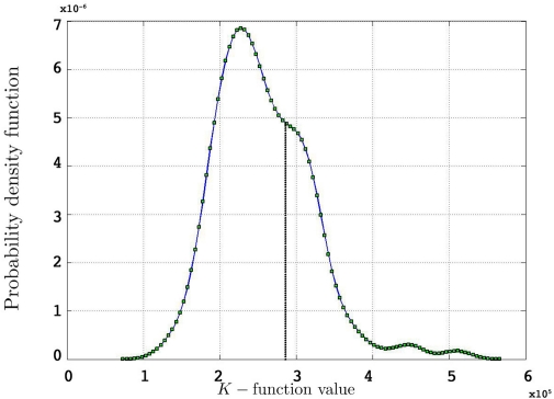
Acquiring a p-value for the two-sided test, would then be a simple matter of locating $\widehat{K}(t)$ on the corresponding probability density function and calculating the area under the curve (see Figure 1).

Figure 1.

Probability density function for 500 simulated K-functions for an arbitrary t and an arbitrary observed value from one of the simulations using the edge correction method in Eq. 11.

Estimating the variance of the K-function using bootstrap

To estimate the variance of the K-functions we adapt the method described by Diggle (2003) to estimate the K-function using replicated data by the bootstrap (Efron and Tibshirani, 1993). Here is how we proceed:

• We introduce the weighted average K-function for each group of point patterns:

$$\widehat{K}(t)=\frac{{\displaystyle {\sum }_{i=1}^r{n}_i{\widehat{K}}_i(t)}}{{\displaystyle {\sum }_{i=1}^r{n}_i}}.$$ (6)

• We create the residual K-function:

$$R_i(t)=\sqrt{n_i}\left({\widehat{K}}_i(t)-\widehat{K}(t)\right):i=1,\mathrm{...},r$$

where r is the number of point patterns in each group.

• The bootstrap sample of K-functions from replicated data is then:

$$K_i^{\ast }(t)=\widehat{K}(t)+\frac{1}{\sqrt{n_i}}{R}_i^{\ast }(t):i=1,\mathrm{...},r$$

where the $R_i^{\ast }(t)$ are chosen randomly with replacement from the set of all R_i(t): i = 1,…,r.

• Finally our estimated K-function from replicated data is:

$${\widehat{K}}^{\ast }(t)=\frac{{\displaystyle {\sum }_{i=1}^r{n}_i{\widehat{K}}_i^{\ast }(t)}}{{\displaystyle {\sum }_{i=1}^r{n}_i}}.$$

This is repeated, say, 1000 times in our applications and results in an equal number of${\widehat{K}}^{\ast }$ -functions for each type/group.

The variance of ${\widehat{K}}^{\ast }(t)$ for different values of t is used as an estimate of V ar$\left(\widehat{K}(t)\right)$.

The lower and upper boundaries of the 95% confidence intervals are then constituted by the 25th smallest and 25th largest $K^{\ast }$ -functions respectively.

Between-group comparisons

In a test for between-group comparisons, the null hypothesis states that the samples of interest follow the same underlying distribution. The test focuses on significant deviations of the estimated K- functions from a weighted average over the entire group/type (Eq. 7) under repeated sampling. This test is argued to be valid even when the underlying intensities of the estimated K-functions vary within or between groups (Diggle, 2003). To start, we let n_ij denote the number of events in sample j in group i, ${\widehat{K}}_{ij}(t)$ the corresponding estimated K-functions and ${\widehat{K}}_i(t)$ the group estimator according to Eq. 6. We define ${\widehat{K}}_0(t)$, our weighted average, as:

$${\widehat{K}}_0(t)=\frac{{\displaystyle {\sum }_i{n}_i{\widehat{K}}_i(t)}}{n}.$$ (7)

The null hypothesis is thus:

$$H_0:K_i(t)=K(t),i=1,\mathrm{...},r$$ (8)

where K(t) is estimated by Eq. 7 and K_i(t) by ${\widehat{K}}_i(t)$. The statistic suggested by Diggle for this hypothesis is:

$$BTSS={\displaystyle {\sum }_{i=1}^r{n}_i{\displaystyle {\int }_0^{t}w(t){\{{\widehat{K}}_i(t)-{\widehat{K}}_0(t)\}}^{2}dt}}$$ (9)

where BTSS is the abbreviation for ‘between-treatment sum of squares’ and w(t) is a weight function (we use w(t) = t⁻² in our applications). This particular choice of weight function is believed to counter the increasing variance of the K-function for increasing values of t in an effective way.

To proceed, we follow a procedure somewhat similar to the one given in Section “Estimating the Variance of the K-function Using Bootstrap”. Having the notations given earlier intact, we define the residual K-function for sample j in group i as:

$$R_{ij}(t)=\sqrt{n_{ij}}\left({\widehat{K}}_{ij}(t)-{\widehat{K}}_i(t)\right):j=1,\mathrm{...},p\hspace{0.17em}\text{and}\hspace{0.17em}i=1,\mathrm{...},r.$$ (10)

We then introduce a set of resampled K-functions under H₀ as

$$K_{ij}^{\ast }(t)={\widehat{K}}_0(t)+\frac{1}{\sqrt{n_{ij}}}{R}_{ij}^{\ast }(t):j=1,\mathrm{...},p\hspace{0.17em}\text{and}\hspace{0.17em}i=1,\mathrm{...},r$$

where $R_{ij}^{\ast }(t)$ is obtainted by random sampling with replacement from the set of R_ij(t):j = 1,…,p and i = 1,…,r. We then establish BTSS_k:k = 1,…,s from the $K_{ij}^{\ast }(t)$ according to Eq. 9 and compare our observed value with this set (using a probablity density function from the resampling). We choose to apply this resampling procedure s = 1000 times where every resampling procedure leads to ${\sum }_{i=1}^r{p}_i$ estimations of bootstrapped K-functions.

Results

Data management

Our interest in this study is to detect deviations from CSR, a model-based study, and to measure the difference between groupwise deviations using inferential statistics, a design-based study using bootstrap.

The brain slice samples are approximately 50-μm thick. Since the analyzed neurons have a cell diameter of 15–20 μm the process of edge correction (see Edge Correction in 3D) is sensitive to false geometrical assumptions. One other challenge here is the non-stationary nature of our samples.

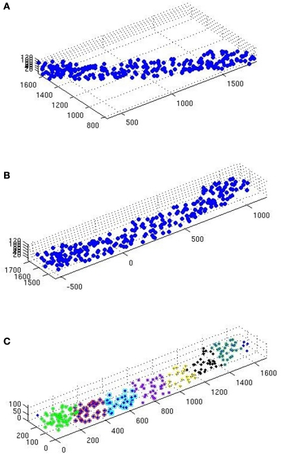
Due to the geometry of the samples the assumption of stationarity is vital for the reliability of our results. Assuming a common underlying process in each group (etv-pyramids and glt-pyramids; Groh et al., 2010) to justify partitioning, the following procedure is meant to enhance the assumption of stationarity (see Figure 2 for a graphic representation of this procedure):

Figure 2.

(A) Scatterplot of a raw glt sample. (B) Same sample after executing the station function. (C) After executing the divide function.

• The samples go through the station function (see station), carrying out 2D rotation transformation, to leave as little ‘empty space’ as possible inside the sample domain.

• The samples are then sent to the divide function (see divide) to be divided in smaller samples (Table 1). The aim here is to obtain even and quadratic domains with respect to the two largest sides (the smallest being that of thickness).

Table 1.

Data Management For the K-function Estimations.

	Number of samples	Number of events in average	x × y × z μm
The properties before running the samples through divide.
etv	5	226	1521 × 280 × 61
glt	6	267	1708 × 329 × 78
The properties after running the samples through divide.
etv	32	33	216 × 163 × 55
glt	37	43	261 × 178 × 70

Due to time efficiency and given that the rotation transformation is performed in 2D, extensive simulations of the K-function in 2D confirmed the satisfactory output of this procedure.

Edge correction in 3D

Edge correction in 3D is vastly different and comes with more limitations than in 2D. The idea is, nevertheless, the same as in 2D where only those parts of a sphere's volume outside the sample domain are measured when evaluating Ripley's K-function according to Eq. 4 in Section “Ripley's K-function”.

Baddeley et al. (1993) proposed three edge correction terms of which the ‘isotropic’ term bears some similarities with the edge correction term we propose in this paper. The ‘isotropic’ edge correction term proposed by Baddeley et al. (1993) is e_i(t) = w(i,j)s(|i − j|),i ≠ j where w(i,j) is an edge correction equal to the proportion of the surface area of the sphere with center at i and radius |i − j| within the sample domain and s(·) is a global geometry correction. The derivation of these terms is demonstrated comprehensively in Baddeley et al. (1993). One distinguishing difference between the ‘isotropic’ edge correction term and the edge correction term outlined in the present paper is the absence of a term treating the surface area of the spherical neighborhoods. Our edge correction operates solely on the volumes of those parts of the spheres outside the sample domain. This and other distinguishing factors between our and the ‘isotropic’ edge correction term are discussed in the Section “Discussion” of this paper.

We establish the following edge correction term for event i with coordinates (x_i,y_i,z_i):

$$e_i(t)=1-\frac{c_i(t)-w_i(t)+s_i(t)}{4\pi t^3/3}.$$ (11)

where c_i(t) is the outside-of-sample volume of a sphere with radius t intercepted by one plane (cap), w_i(t) is the outside-of-sample volume of a wedge caused by the interception of two planes and s_i(t) is the outside-of-sample volume of a semi-wedge caused by the interception of three planes. These volumes are calculated using analytical formulas and integrals where the latter are computed numerically by the quad function in MATLAB.

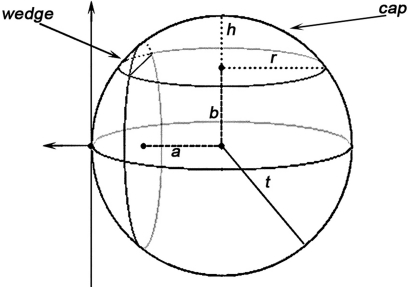
Volume of a cap, using the notations in Figure 3, is evaluated according to:

Figure 3.

A demonstration of how caps and wedges may occur where a and b are the Euclidean distances from the event to the sample domain boundaries, t is the radius of the sphere as in K(t), and h and r are the height and radius of the outside-of-domain cap respectively.

$$V_{\text{cap}}=\frac{(\pi h)(3r^2+h^2)}{6}.$$

As for a wedge, using the notations in Figure 3:

$$V_{\text{wedge}}\text{= }{\displaystyle {\int }_a^{\sqrt{t^2-b^2}}{\displaystyle {\int }_{-{\left(\sqrt{t^2-(a^2+b^2)}\right)}^{+}}^{+{\left(\sqrt{t^2-(a^2+b^2)}\right)}^{+}}{\left(\sqrt{t^2-(u^2+v^2)}-b\right)}^{+}\text{d}u\text{d}v}}\text{.}$$

Semi-wedges occur when the spherical neighborhood is centered around an event in the corner of the domain. Taking these semi-wedges into our calculations would liberate us from eliminating the corner-events and naturally increase the number of events to be observed and thus enhance the edge correction term in accuracy. The cost-benefit analysis here is, however, subjective and depends primarily on the geometry of samples and the contribution of corner events to the overall accuracy, and the performance of the computing device. The volume of a semi-wedge can be expressed by:

$$V_{\text{semi-wedge}}={\displaystyle {\int }_a^{\sqrt{t^2-b^2}}{\displaystyle {\int }_{-{\left(\sqrt{t^2-(a^2+b^2)}\right)}^{+}}^g{\left(\sqrt{t^2-(u^2+v^2)}-b\right)}^{+}\text{d}u\text{d}v}}$$

where, keeping the notations of Figure 3 intact, g is the Euclidean distance from the center of the sphere to a plane, parallel to the page, cutting the sphere. The edge correction term in Eq. 11 is outlined in details in the Section “The Edge Correction Term” in Appendix.

Thus, the edge correction term e_i(t) in Eq. 11 consists of 6 possible analytical terms and 20 possible integral terms of which 12 are wedge volumes and 8 are semi-wedge volumes. The computational efficiency of this method depends, to a large extent, on a few intuitively obvious factors such as the upper limit of t, the number of events in the sample and the performance of the computing device.

Simulations

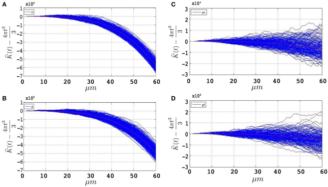
Figures 4A,B represent the obtained $\widehat{K}(t)-4\pi t^3/3$ plots from simulations of under CSR without any edge correction term. Figures 4C,D represent the simulations with the edge correction term in Eq. 11. The geometries of the sample domains are identical to the samples used in the 3D application after executing the steps in Section “Data Management”. Clearly, the absence of an edge correction term results in a display of inhibition by the K- function as it regards the ‘empty space’ outside the sample domain as a part of the domain. The simulation results in Figure 4 confirm the satisfactory performance of the established edge correction term where the K-function estimations subtracted by the expected value (4πt³/3) are expected to be centered around 0.

Figure 4.

500 estimations of the K-function based on simulations under CSR for samples identical in geometry to etv-pyramids (A,C) and glt-pyramids (B,D). The simulations demonstrate the expected outcome when estimating the K-function without (A,B) and with (C,D) the edge correction term under CSR (having $\widehat{K}(t)-4\pi t^3/3$ on the y-axis).

Note that the K-function has been evaluated for t = 0,…,60 μm. Ripley (1987), Diggle (2003) and Costa et al. (2007) recommend a maximum threshold for t equal to the 0.25 of the shortest side length. This is partially the reason why we use simulations to have an understanding of how t-values larger than the one recommended influence the outcome of the K-function. How exceeding the recommended threshold for t influences our results and interpretation is outlined in the Section “Discussion”.

Analysis of the mouse brain data

K-function estimations

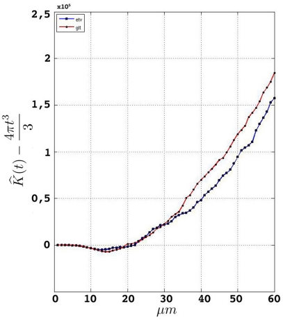
Having performed the steps in Section “Data Management” and established a consistent edge correction term, the samples fulfill the prerequisites to be analyzed by Ripley's K-function. Figure 5 represents the estimated K-function values subtracted by its expected value $(\widehat{K}(t)-4\pi t^3/3)$ for etv- and glt-pyramids. Values larger than zero given by $\widehat{K}(t)-4\pi t^3/3$ suggest aggregated underlying point patterns.

Figure 5.

Groupwise average (weighted) $\widehat{K}(\text{t})-4\pi {\text{t}}^3/3$ for samples in etv-pyramids and glt-pyramids.

Hypothesis tests of CSR

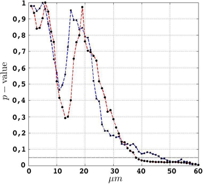
In order to investigate the significance of the observed deviations from CSR, the p-values from the hypothesis tests of CSR, the two-sided null hypothesis in Eq. 5, obtainted from 500 CSR point pattern simulations, are given in the table below. Figure 6 present an arguably more useful representation of these p-values.

Figure 6.

etv (blue) and glt (red) p-values for different values of t. The drop for values larger than 10 μm translates well to cell diameters of 15–20 μm.

t	etv	glt
20 μm	0.7837	0.7607
30 μm	0.1744	0.2839
40 μm	0.0754	0.0323
50 μm	0.0230	0.0204
60 μm	0.0060	0.0046

Given that the results obtained from the simulations allow more variance for larger values of t, the etv- and glt-pyramids display significant tendencies towards clustering for values larger than t = 47 μm and t = 38 μm, respectively. Loosely interpreted in a geometrical sense, this expresses a more intense clustering in glt-pyramid samples, or alternatively, a higher frequency of empty spaces in the spatial point pattern underlying the glt-pyramids.

To investigate the fact that the glt-pyramids incline towards significant aggregation at lower values of t than the etv-pyramids, we will employ the BTSS statistic presented in Between-group Comparisons in Section “Between-group Comparisons”.

Estimating the variance of the K-functions

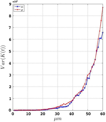
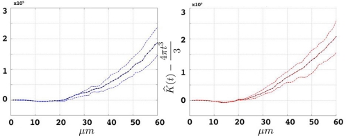
We estimate the variance of the underlying K-functions applying the theoretical framework presented in Section “Estimating the Variance of the K-function Using Bootstrap”. Figure 7 represents the variance of the estimated K-functions based on bootstrap resampling. The figure illustrates rather similiar variance functions for etv- and glt pyramids which is reasonable (but not necessary) justification to compare these two groups using the BTSS statistic outlined in Section “Between-group Comparisons”. The estimated variance is also used to establish confidence intervals as seen in Figure 8.

Figure 7.

Estimated variance of $\widehat{K}(\text{t})$ for etv and glt.

Figure 8.

Groupwise average (weighted) $\widehat{K}(t)-4\pi t^3/3$ for etv- (left) and glt-pyramids (right) and confidence intervals based on the bootstrap procedure (dashed).

Between-group comparisons

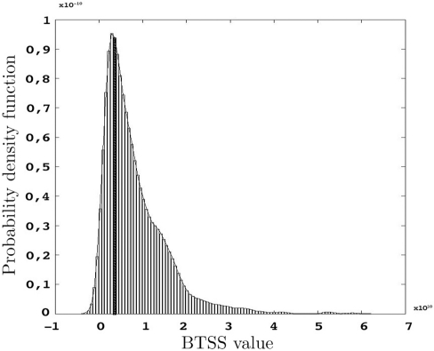
The p-values represented below are obtained using the test statistic BTSS and the weight function w(t) = t⁻² as represented in Eq. 8 in Section “Between-group Comparisons”. The probability density function of the BTSS test is represented in Figure 9. A look at the long-tailed density function reveals the large variance of this test statistic. This large variance corresponds to the large variability of the samples in the etv- and glt-pyramids which produce a test sensitive only to relatively large between-group deviations; hence the large p-values.

Figure 9.

Probability density function of BTSS for s = 1000 resamples and the observed BTSS (filled bar) when w(t) = t⁻² and t= 20,…,60 μm.

t	p-value
[0..60]	0.7288
[20..60]	0.7281
[30..60]	0.7721
[40..60]	0.7521

Conclusion

The analysis in general reveals the aggregated point pattern distribution of the etv- and glt-pyramid samples. This aggregation is significant for values greater than 47 μm among the etv-pyramids and values over 38 μm among the glt-pyramids. The seemingly stronger inclination of glt-pyramids to demonstrate aggregated behavior is, however, insignificant.

Discussion

We present a framework in which Ripley's K-function and a corresponding edge correction term can be used to analyze the spatial distribution of events (such as neurons) in 3D space. We exemplify the use of this method by analyzing the distribution of genetically labeled layer 5 pyramidal cells in mouse somatosensory barrel cortex.

The assumption of stationarity after adjusting and dividing the initial samples into smaller ones turned out to be very solid. This is, as emphasized earlier, a very important corner stone of our theoretical design when we wish to use a constant intensity in the estimation of the K-function. The assumption of isotropy, however, was believed to be fulfilled in the default setting of the samples. Employing the K-function in a global form implies establishing a solid edge correction term to avoid underestimating the number of events in the underlying point patterns. The edge correction term in Eq. 11 is constructed to neutralize the false assumption of point pattern vacancy when the observed space is outside the sample domain. The correction is done for every single event at a range of distance values, t, and is therefore called a local edge correction term (not to be confused with the local (non-domain exceeding) form of Ripley's K-function). By subtracting the volumes outside the domain, the edge correction term determines what proportions of the spherical neighborhoods are inside the domain. A large part of these volumes are evaluated using numerical methods in MATLAB (the quad function).

The edge correction method outlined in the present paper bears some similarities in its theoretical design to the ‘isotropic’ edge correction term described by Baddeley et al. (1993) [and subsequently applied in Eglen et al. (2008)]. The differences, however, are firstly that our approach produces the volume integrals directly from the theoretical framework without any transformations or other intermediate calculations. Secondly, in contrast to the ‘isotropic’ edge correction method we do not need to include a term for the proportion of the surface area in the edge correction term. Our edge correction term is consistent and leads to an unbiased estimate of the K-function according to the simulations. An improvement of the correction term could be made along the lines established by Ward and Ferrandino (1999), where the edge correction term is evaluated globally for each value of t.

The recommendation on what maximum value of t is reasonable to employ in the estimation of the K-function (Ripley, 1987; Diggle, 2003), is an additional reason why we use simulations to have an understanding of how t-values larger than the one recommended influence the outcome of the K-function. For this purpose, the simulations were done on two sets (500 samples in each) of samples constituted of Poisson-distributed spatial point patterns. These simulated samples follow the same geometry and point pattern intensity of the etv- and glt-samples on which we conducted the analyses. What is observed is that as the value of t increases, the K-function tends to indicate inhibition (Figures 4A,B). Bearing this tendency to inhibition for large t-values in mind, and given that the K-functions obtained from the analysis on the etv- and glt-samples indicate aggregation, we draw the conclusion that using the K-function for values larger than 15 μm (which in for these data samples is 0.25 of the shortest sample side), although arguably inconsistent, does not lead to an erroneous indication of aggregation. If anything, the aggregation is rather underestimated. Additionally, given what is biologically relevant and interesting (the cell diameter itself is 15–20 μm), t-values smaller than 15 μm do not deliver any result of interest in the present case.

The analysis of the 3D-distribution of specifically labeled neuron populations will be an important contribution to the characterization of neuronal types and for studying structure-function relationships. The mouse brain samples investigated in the present study were from the somatosensory barrel cortex and contained cells expressing the fluorescent protein EGFP under the control of a cell-type specific promoter (Gong et al., 2003). The two different cell types labeled were glt-expressing layer 5 pyramidal neurons projecting to thalamus and pons (corticothalamic/pontine cells), and etv-expressing layer 5 pyramidal neurons projecting to striatum (corticostriatal cells; Groh et al., 2010). Using Ripley's K-function adapted to 3D we show that the spatial distribution of the two cell types was largely similar with a significant clustering for t values around 40 μm. Although a tendency was observed for more clustering of corticothalamic/pontine (glt-pyramids) compared to corticostriatal cells (etv-pyramids). The larger tendency for clustering of the glt-pyramids in lower layer 5 (the so called, layer 5B) is probably due to a partial overlap between the glt-expressing population and the genetically labeled layer 5B population described in Krieger et al. (2007), where the pyramidal neurons were arranged in cell groups having bundling dendrites. Interestingly the significant clustering appears at t-values in the range of the expected spacing between minicolumns (White and Peters, 1993; Krieger et al., 2007). The emphasis in the present project was to develop a practical tool to study the spatial distribution in 3D, thus a full investigation of the spatial distribution of neurons would require a larger data sample covering the whole extent of the barrel column to account for variations in the cell density within a barrel column (White and Peters, 1993).

In a broader perspective, the emergence of high-resolution 3D digital atlases and tools for 3D morphological reconstructions elucidating various underlying biological structures necessitates the implementation of consistent analytical methodologies in order to utilize the output of these reconstructions in the most optimal way (Allen Brain Atlas¹; GENSAT²; Kötter, 2001; Briggman and Denk, 2006; Hjornevik et al., 2007; Martone et al., 2008; Mailly et al., 2009; Oberlaender et al., 2009). Ripley's K-function and its corresponding inferential designs using bootstrap re-sampling is one such methodology for analyzing the spatial distribution of neurons and neuronal processes having the advantage that it is theoretically fairly simple and practically reasonably intuitive.

Conflict of Interest Statement

The authors declare that the research was conducted in the absence of any commercial or financial relationships that could be construed as a potential conflict of interest.

Appendix

Appendix

Data management

Station

The station function is based on the two following 2D rotation matrices:

$$R_{\text{cw}}(\text{θ})=\left(\begin{array}{cc}\text{cos}\hspace{0.17em}\text{θ}& \text{sin}\hspace{0.17em}\text{θ}\\ \text{sin}\hspace{0.17em}\text{θ}& -\text{cos}\hspace{0.17em}\text{θ}\end{array}\right)\hspace{0.17em}\text{and}\hspace{0.17em}{R}_{\text{ccw}}(\theta )=\left(\begin{array}{cc}\text{cos}\hspace{0.17em}\text{θ}& -\text{sin}\hspace{0.17em}\text{θ}\\ \text{sin}\hspace{0.17em}\text{θ}& \text{cos}\hspace{0.17em}\text{θ}\end{array}\right)$$

The 2D rotation is even applied to 3D data due to the slight thickness of samples in this paper. The function recognizes the thickness dimension (we choose to call this dimension z) automatically as the dimension with the smallest span of coordinates, and performs a 2D rotation if the angle constituted by the diagonal on the xy-plane and the longest edge exceeds theta degrees. The output is a new set of coordinates constituting a domain which fulfills the assumption of stationarity and a 2D scatter-plot that shows the data before and after the 2D rotation on the xy-plane.

Divide

This function divides the initial 2D set of coordinates into subsets where the width and length of the domains embodying the new subsets is as equal as possible. The goal, in other words, is to create quadratically shaped subsets on the 2D plane.

The edge correction term

We introduce the following notations for an arbitrary event i with coordinates (x_i,y_i,z_i):

dx_min = |x_i − x_min|

dx_max = |x_i − x_max|

dy_min = |y_i − y_min|

dy_max = |y_i − y_max|

dz_min = |z_i − z_min|

dz_max = |z_i − z_max|

where x_min, for instance, represents the lower sample domain boundary along the x-axis and x_max its corresponding upper boundary.

We establish the following edge correction term for event i with coordinates (x_i,y_i,z_i):

$$e_i(t)=1-\frac{c_i(t)-w_i(t)+s_i(t)}{4\pi t^3/3}.$$

where c_i(t) is the outside-of-sample volume of a sphere with radius t intercepted by one plane (that is volume of the cap outside the sample domain), w_i(t) is the outside-of-sample volume of a wedge caused by the interception of two planes and s_i(t) is the outside-of-sample volume of a semi-wedge caused by the interception of three planes.

The term c_i(t) expands to:

$$\begin{array}{c}{c}_i(t)=c_i^x(t)+c_i^y(t)+c_i^z(t)\\ =c_i^{x_{\text{min}}}(t)+c_i^{x_{\text{max}}}(t)+c_i^{y_{\text{min}}}(t)+c_i^{y_{\text{max}}}(t)+c_i^{z_{\text{min}}}(t)+c_i^{z_{\text{max}}}(t)\\ =\frac{\pi \left(t-\text{d}{x}_{\text{min}}\right)\cdot \left(3\left(t^2-\text{d}{x}_{\min }^2\right)+{\left(t-\text{d}{x}_{\text{min}}\right)}^2\right)}{6}\\ \hspace{0.17em}\hspace{0.17em}\hspace{0.17em}+\frac{\pi \left(t-\text{d}{x}_{\text{max}}\right)\cdot \left(3\left(t^2-\text{d}{x}_{\max }^2\right)+{\left(t-\text{d}{x}_{\text{max}}\right)}^2\right)}{6}\\ \hspace{0.17em}\hspace{0.17em}\hspace{0.17em}+\frac{\pi \left(t-\text{d}{y}_{\text{min}}\right)\cdot \left(3\left(t^2-\text{d}{y}_{\min }^2\right)+{\left(t-\text{d}{y}_{\text{min}}\right)}^2\right)}{6}\\ \hspace{0.17em}\hspace{0.17em}\hspace{0.17em}+\frac{\pi \left(t-\text{d}{y}_{\text{max}}\right)\cdot \left(3\left(t^2-\text{d}{y}_{\max }^2\right)+{\left(t-\text{d}{y}_{\text{max}}\right)}^2\right)}{6}\\ \hspace{0.17em}\hspace{0.17em}\hspace{0.17em}+\frac{\pi \left(t-\text{d}{z}_{\text{min}}\right)\cdot \left(3\left(t^2-\text{d}{z}_{\min }^2\right)+{\left(t-\text{d}{z}_{\text{min}}\right)}^2\right)}{6}\\ \hspace{0.17em}\hspace{0.17em}\hspace{0.17em}\hspace{0.17em}+\frac{\pi \left(t-\text{d}{z}_{\text{max}}\right)\cdot \left(3\left(t^2-\text{d}{z}_{\max }^2\right)+{\left(t-\text{d}{z}_{\text{max}}\right)}^2\right)}{6}.\end{array}$$

Likewise w_i(t) is expanded to:

$$\begin{array}{c}{w}_i(t)=w_i^{xy}(t)+w_i^{xz}(t)+w_i^{yz}(t)\\ =w_i^{x_{\text{min}}{y}_{\text{min}}}(t)+w_i^{x_{\text{min}}{y}_{\text{max}}}(t)+w_i^{x_{\text{max}}{y}_{\text{min}}}(t)+w_i^{x_{\text{max}}{y}_{\text{max}}}(t)\\ \hspace{0.17em}+w_i^{x_{\text{min}}{z}_{\text{min}}}(t)+w_i^{x_{\text{min}}{z}_{\text{max}}}(t)+w_i^{x_{\text{max}}{z}_{\text{min}}}(t)+w_i^{x_{\text{max}}{z}_{\text{max}}}(t)\\ \hspace{0.17em}+w_i^{y_{\text{min}}{z}_{\text{min}}}(t)+w_i^{y_{\text{min}}{z}_{\text{max}}}(t)+w_i^{y_{\text{max}}{z}_{\text{min}}}(t)+w_i^{y_{\text{max}}{z}_{\text{max}}}(t)\\ ={\displaystyle {\int }_{\text{d}{x}_{\min }}^{\sqrt{t^2-\text{d}{y}_{\min }^2}}{\displaystyle {\int }_{-{\left(\sqrt{t^2-(\text{d}{x}_{\min }^2+\text{d}{y}_{\min }^2)}\right)}^{+}}^{+{\left(\sqrt{t^2-(\text{d}{x}_{\min }^2+\text{d}{y}_{\min }^2)}\right)}^{+}}{\left(\sqrt{t^2-(u^2+v^2)}-\text{d}{y}_{\min }\right)}^{+}dudv}}\\ +{\displaystyle {\int }_{\text{d}{x}_{\min }}^{\sqrt{t^2-\text{d}{y}_{\max }^2}}{\displaystyle {\int }_{-{\left(\sqrt{t^2-(\text{d}{x}_{\min }^2+\text{d}{y}_{\max }^2)}\right)}^{+}}^{+{\left(\sqrt{t^2-(\text{d}{x}_{\min }^2+\text{d}{y}_{\max }^2)}\right)}^{+}}{\left(\sqrt{t^2-(u^2+v^2)}-\text{d}{y}_{\max }\right)}^{+}\text{d}u\text{d}v}}\\ +{\displaystyle {\int }_{\text{d}{x}_{\max }}^{\sqrt{t^2-\text{d}{y}_{\min }^2}}{\displaystyle {\int }_{-{\left(\sqrt{t^2-(\text{d}{x}_{\max }^2+\text{d}{y}_{\min }^2)}\right)}^{+}}^{+{\left(\sqrt{t^2-(\text{d}{x}_{\max }^2+\text{d}{y}_{\min }^2)}\right)}^{+}}{\left(\sqrt{t^2-(u^2+v^2)}-\text{d}{y}_{\min }\right)}^{+}\text{d}u\text{d}v}}\\ +{\displaystyle {\int }_{\text{d}{x}_{\max }}^{\sqrt{t^2-\text{d}{y}_{\max }^2}}{\displaystyle {\int }_{-{\left(\sqrt{t^2-(\text{d}{x}_{\max }^2+\text{d}{y}_{\max }^2)}\right)}^{+}}^{+{\left(\sqrt{t^2-(\text{d}{x}_{\max }^2+\text{d}{y}_{\max }^2)}\right)}^{+}}{\left(\sqrt{t^2-(u^2+v^2)}-\text{d}{y}_{\max }\right)}^{+}\text{d}u\text{d}v}}\\ +{\displaystyle {\int }_{\text{d}{x}_{\min }}^{\sqrt{t^2-\text{d}{z}_{\min }^2}}{\displaystyle {\int }_{-{\left(\sqrt{t^2-(\text{d}{x}_{\min }^2+\text{d}{z}_{\min }^2)}\right)}^{+}}^{+{\left(\sqrt{t^2-(\text{d}{x}_{\min }^2+\text{d}{z}_{\min }^2)}\right)}^{+}}{\left(\sqrt{t^2-(u^2+v^2)}-\text{d}{z}_{\min }\right)}^{+}\text{d}u\text{d}v}}\\ +{\displaystyle {\int }_{\text{d}{x}_{\min }}^{\sqrt{t^2-\text{d}{z}_{\max }^2}}{\displaystyle {\int }_{-{\left(\sqrt{t^2-(\text{d}{x}_{\min }^2+\text{d}{z}_{\max }^2)}\right)}^{+}}^{+{\left(\sqrt{t^2-(\text{d}{x}_{\min }^2+\text{d}{z}_{\max }^2)}\right)}^{+}}{\left(\sqrt{t^2-(u^2+v^2)}-\text{d}{z}_{\max }\right)}^{+}\text{d}u\text{d}v}}\\ +{\displaystyle {\int }_{d{x}_{\max }}^{\sqrt{t^2-\text{d}{z}_{\min }^2}}{\displaystyle {\int }_{-{\left(\sqrt{t^2-(\text{d}{x}_{\max }^2+\text{d}{z}_{\min }^2)}\right)}^{+}}^{+{\left(\sqrt{t^2-(\text{d}{x}_{\max }^2+\text{d}{z}_{\max }^2)}\right)}^{+}}{\left(\sqrt{t^2-(u^2+v^2)}-\text{d}{z}_{\min }\right)}^{+}\text{d}u\text{d}v}}\\ +{\displaystyle {\int }_{\text{d}{x}_{\max }}^{\sqrt{t^2-\text{d}{z}_{\max }^2}}{\displaystyle {\int }_{-{\left(\sqrt{t^2-(\text{d}{x}_{\max }^2+\text{d}{z}_{\max }^2)}\right)}^{+}}^{+{\left(\sqrt{t^2-(\text{d}{x}_{\max }^2+\text{d}{z}_{\max }^2)}\right)}^{+}}{\left(\sqrt{t^2-(u^2+v^2)}-\text{d}{z}_{\max }\right)}^{+}\text{d}u\text{d}v}}\\ +{\displaystyle {\int }_{\text{d}{y}_{\min }}^{\sqrt{t^2-\text{d}{z}_{\min }^2}}{\displaystyle {\int }_{-{\left(\sqrt{t^2-(\text{d}{y}_{\min }^2+\text{d}{z}_{\min }^2)}\right)}^{+}}^{+{\left(\sqrt{t^2-(\text{d}{y}_{\min }^2+\text{d}{z}_{\min }^2)}\right)}^{+}}{\left(\sqrt{t^2-(u^2+v^2)}-\text{d}{z}_{\min }\right)}^{+}\text{d}u\text{d}v}}\\ +{\displaystyle {\int }_{\text{d}{y}_{\min }}^{\sqrt{t^2-\text{d}{z}_{\max }^2}}{\displaystyle {\int }_{-{\left(\sqrt{t^2-(\text{d}{y}_{\min }^2+\text{d}{z}_{\max }^2)}\right)}^{+}}^{+{\left(\sqrt{t^2-(\text{d}{y}_{\min }^2+\text{d}{z}_{\max }^2)}\right)}^{+}}{\left(\sqrt{t^2-(u^2+v^2)}-\text{d}{z}_{\max }\right)}^{+}\text{d}u\text{d}v}}\\ +{\displaystyle {\int }_{\text{d}{y}_{\max }}^{\sqrt{t^2-\text{d}{z}_{\min }^2}}{\displaystyle {\int }_{-{\left(\sqrt{t^2-(\text{d}{y}_{\max }^2+\text{d}{z}_{\min }^2)}\right)}^{+}}^{+{\left(\sqrt{t^2-(\text{d}{y}_{\max }^2+\text{d}{z}_{\min }^2)}\right)}^{+}}{\left(\sqrt{t^2-(u^2+v^2)}-\text{d}{z}_{\min }\right)}^{+}\text{d}u\text{d}v}}\\ +{\displaystyle {\int }_{\text{d}{y}_{\max }}^{\sqrt{t^2-\text{d}{z}_{\max }^2}}{\displaystyle {\int }_{-{\left(\sqrt{t^2-(\text{d}{y}_{\max }^2+\text{d}{z}_{\max }^2)}\right)}^{+}}^{+{\left(\sqrt{t^2-(\text{d}{y}_{\max }^2+\text{d}{z}_{\max }^2)}\right)}^{+}}{\left(\sqrt{t^2-(u^2+v^2)}-\text{d}{z}_{\max }\right)}^{+}\text{d}u\text{d}v.}}\end{array}$$

The semi-wedge volumes can be expressed by:

$$\begin{array}{c}{s}_i(t)=s_i^{x_{\text{min}}{y}_{\text{min}}{z}_{\text{min}}}(t)+s_i^{x_{\text{min}}{y}_{\text{min}}{z}_{\text{max}}}(t)+s_i^{x_{\text{min}}{y}_{\text{max}}{z}_{\text{min}}}(t)\\ \hspace{0.17em}\hspace{0.17em}+s_i^{x_{\text{min}}{y}_{\text{max}}{z}_{\text{max}}}(t)+s_i^{x_{\text{max}}{y}_{\text{min}}{z}_{\text{min}}}(t)+s_i^{x_{\text{max}}{y}_{\text{min}}{z}_{\text{max}}}(t)\\ \hspace{0.17em}\hspace{0.17em}\hspace{0.17em}+s_i^{x_{\text{max}}{y}_{\text{max}}{z}_{\text{min}}}(t)+s_i^{x_{\text{max}}{y}_{\text{max}}{z}_{\text{max}}}(t)\\ ={{\displaystyle {\int }_{\text{d}{x}_{\text{min}}}^{\sqrt{t^2-\text{d}{y}_{\min }^2}}{\displaystyle {\int }_{+\text{d}{z}_{\text{min}}}^{+{\left(\sqrt{t^2-(\text{d}{x}_{\min }^2+\text{d}{y}_{\min }^2)}\right)}^{+}}\left(\sqrt{t^2-(u^2+v^2)}-\text{d}{y}_{\text{min}}\right)}}}^{+}\text{d}u\text{d}v\\ +{{\displaystyle {\int }_{\text{d}{x}_{\text{min}}}^{\sqrt{t^2-\text{d}{y}_{\min }^2}}{\displaystyle {\int }_{-{\left(\sqrt{t^2-(\text{d}{x}_{\min }^2+\text{d}{y}_{\min }^2)}\right)}^{+}}^{-\text{d}{z}_{\text{max}}}\left(\sqrt{t^2-(u^2+v^2)}-\text{d}{y}_{\text{min}}\right)}}}^{+}\text{d}u\text{d}v\\ +{{\displaystyle {\int }_{\text{d}{x}_{\text{min}}}^{\sqrt{t^2-\text{d}{y}_{\max }^2}}{\displaystyle {\int }_{+\text{d}{z}_{\text{min}}}^{+{\left(\sqrt{t^2-(\text{d}{x}_{\min }^2+\text{d}{y}_{\max }^2)}\right)}^{+}}\left(\sqrt{t^2-(u^2+v^2)}-\text{d}{y}_{\text{max}}\right)}}}^{+}\text{d}u\text{d}v\\ +{{\displaystyle {\int }_{\text{d}{x}_{\text{min}}}^{\sqrt{t^2-\text{d}{y}_{\max }^2}}{\displaystyle {\int }_{-{\left(\sqrt{t^2-(\text{d}{x}_{\min }^2+\text{d}{y}_{\max }^2)}\right)}^{+}}^{-\text{d}{z}_{\text{max}}}\left(\sqrt{t^2-(u^2+v^2)}-\text{d}{y}_{\text{max}}\right)}}}^{+}\text{d}u\text{d}v\\ +{{\displaystyle {\int }_{\text{d}{x}_{\text{max}}}^{\sqrt{t^2-\text{d}{y}_{\min }^2}}{\displaystyle {\int }_{+\text{d}{z}_{\text{min}}}^{+{\left(\sqrt{t^2-(\text{d}{x}_{\max }^2+\text{d}{y}_{\min }^2)}\right)}^{+}}\left(\sqrt{t^2-(u^2+v^2)}-\text{d}{y}_{\text{min}}\right)}}}^{+}\text{d}u\text{d}v\\ +{{\displaystyle {\int }_{\text{d}{x}_{\text{max}}}^{\sqrt{t^2-\text{d}{y}_{\min }^2}}{\displaystyle {\int }_{-{\left(\sqrt{t^2-(\text{d}{x}_{\max }^2+\text{d}{y}_{\min }^2)}\right)}^{+}}^{-\text{d}{z}_{\text{max}}}\left(\sqrt{t^2-(u^2+v^2)}-\text{d}{y}_{\text{min}}\right)}}}^{+}\text{d}u\text{d}v\\ +{{\displaystyle {\int }_{\text{d}{x}_{\text{max}}}^{\sqrt{t^2-\text{d}{y}_{\max }^2}}{\displaystyle {\int }_{+d{z}_{\text{min}}}^{+{\left(\sqrt{t^2-(\text{d}{x}_{\max }^2+\text{d}{y}_{\max }^2)}\right)}^{+}}\left(\sqrt{t^2-(u^2+v^2)}-\text{d}{y}_{\text{max}}\right)}}}^{+}\text{d}u\text{d}v\\ +{{\displaystyle {\int }_{\text{d}{x}_{\text{max}}}^{\sqrt{t^2-\text{d}{y}_{\max }^2}}{\displaystyle {\int }_{-{\left(\sqrt{t^2-(\text{d}{x}_{\max }^2+\text{d}{y}_{\max }^2)}\right)}^{+}}^{-d{z}_{\text{max}}}\left(\sqrt{t^2-(u^2+v^2)}-\text{d}{y}_{\text{max}}\right)}}}^{+}\text{d}u\text{d}v.\end{array}$$

Implementing the first semi-wedge integral in MATLAB for a given t, given that (t>dxmin && t>dymin && t>dzmin), corresponds to:

i = sqrt(t^2−dymin^2−dxmin^2)*(t^2−dymin^2−dxmin^2>0);

F = @(x,y)(sqrt(t.^2−(x.^2 + y.^2))−dymin). *(t.^2−x.^2−y.^2< = dymin^2);

Vol_sw = dblquad(F,dzmin,i,dxmin,sqrt (t^2−dymin^2),tol);

where tol is a specified tolerance degree in the numerical evaluation by the function dblquad.

References

- Baddeley A. J., Moyeed R. A., Howard C. V., Boyde A. (1993). Analysis of a three-dimensional point pattern with replication. J. R. Stat. Soc. 42, 641–668 [Google Scholar]
- Beil M., Fleischer F., Schmidt V. (2005). Statistical analysis of the three-dimensional structure of centromeric heterochromatin in interphase nuclei. J. Microsc. 217, 60–68 10.1111/j.0022-2720.2005.01439.x [DOI] [PubMed] [Google Scholar]
- Bjaalie J. G., Diggle P. J., Nikundiwe A., Karagülle T., Brodal P. (1991). Spatial segregation between populations of ponto-cerebellar neurons. Statistical analysis of multivariate spatial interactions. Anat. Rec. 231, 510–523 10.1002/ar.1092310413 [DOI] [PubMed] [Google Scholar]
- Briggman K. L., Denk W. (2006). Towards neural circuit reconstruction with volume electron microscopy techniques. Curr. Opin. Neurobiol. 6, 562–570 10.1016/j.conb.2006.08.010 [DOI] [PubMed] [Google Scholar]
- Buxhoeveden D. P., Switala A. E., Roy E., Casanova M. F. (2000). Quantitative analysis of cell columns in the cerebral cortex. J. Neurosci. Methods 97, 7–17 10.1016/S0165-0270(99)00192-2 [DOI] [PubMed] [Google Scholar]
- Costa L., da F., Bonci D. M. O., Saito C. A., Rocha F. A., de F., Silveira L. C., de L., Ventura D. F. (2007). Voronoi analysis uncovers relationship between mosaics of normally placed and displaced amacrine cells in the thraira retina. Neuroinformatics 5, 59–78 [DOI] [PubMed] [Google Scholar]
- da Silva E. C., Silva A. C., de Paiva A. C., Nunes R. A., Gattass M. (2008). Diagnosis of solitary lung nodules using the local form of Ripley's K function applied to three-dimensional CT data. Comput. Methods Programs Biomed. 90, 230–239 10.1016/j.cmpb.2008.02.003 [DOI] [PubMed] [Google Scholar]
- Diggle P. J. (1986). Displaced amacrine cells in the retina of a rabbit: analysis of a bivariate spatial point pattern. J. Neurosci. Methods 18, 115–125 10.1016/0165-0270(86)90115-9 [DOI] [PubMed] [Google Scholar]
- Diggle P. J. (2003). Statistical Analysis of Spatial Point Patterns New York: Oxford University Press Inc [Google Scholar]
- Doguwa S. I., Upton G. J. G. (1988). Edge-corrected estimators for the reduced second moment measure of point processes. Biom. J. 31, 563–575 10.1002/bimj.4710310509 [DOI] [Google Scholar]
- Duyckaerts C., Godefroy G. (2000). Voronoi tessellation to study the numerical density and the spatial distribution of neurons. J. Chem. Neuroanat. 20, 83–92 10.1016/S0891-0618(00)00064-8 [DOI] [PubMed] [Google Scholar]
- Duyckaerts C., Godefroy G., Hauw J.-J. (1994). Evaluation of neuronal numerical density by Dirichlet tessellation. J. Neurosci. Methods 51, 47–69 10.1016/0165-0270(94)90025-6 [DOI] [PubMed] [Google Scholar]
- Efron B., Tibshirani R. J. (1993). An Introduction to the Bootstrap New York: Chapman & Hall [Google Scholar]
- Eglen S. J., Lofgreen D. D., Raven M. A., Reese B. E. (2008). Analysis of spatial relationships in three dimensions: tools for the study of nerve cell patterning. BMC Neurosci. 9, 68. 10.1186/1471-2202-9-68 [DOI] [PMC free article] [PubMed] [Google Scholar]
- Gong S., Zheng C., Doughty M. L., Losos K., Didkovsky N., Schambra U. B., Nowak N. J., Joyner A., Leblanc G., Hatten M. E., Heintz N. (2003). A gene expression atlas of the central nervous system based on bacterial artificial chromosomes. Nature 425, 917–925 10.1038/nature02033 [DOI] [PubMed] [Google Scholar]
- Groh A., Krieger P. (2010). “Structure-function analysis of genetically defined neuronal populations,” in Optical Imaging in Neuroscience: A Laboratory Manual. eds Yuste R., Konnerth A., Helmchen F. (New York: CSHL Press; ). [Google Scholar]
- Groh A., Meyer H. S., Schmidt E., Heintz N., Sakmann B., Krieger P. (2010). Cell-type specific properties of pyramidal neurons in neocortex underlying a layout that is modifiable depending on the cortical area. Cereb. Cortex 20, 826–36 Epub. 2009 Jul 30. 10.1093/cercor/bhp152 [DOI] [PubMed] [Google Scholar]
- Hjornevik T., Leergaard T. B., Darine D., Moldestad O., Dale A. M., Willoch F., Bjaalie J. G. (2007). Three-dimensional atlas system for mouse and rat brain imaging data. Front. Neuroinformatics 1, 4. 10.3389/neuro.11/004.2007 [DOI] [PMC free article] [PubMed] [Google Scholar]
- Illian J., Penttinen A., Stoyan H., Stoyan D. (2008). Statistical Analysis and Modelling of Spatial Point Patterns. (Wiley-Interscience). [Google Scholar]
- Kötter R. (2001). Neuroscience databases: tools for exploring brain structure-function relationships. Philos. Trans. R. Soc. Lond., B, Biol. Sci. 356, 1111–1120 10.1098/rstb.2001.0902 [DOI] [PMC free article] [PubMed] [Google Scholar]
- Krieger P., Kuner T., Sakmann B. (2007). Synaptic connections between layer 5B pyramidal neurons in mouse somatosensory cortex are independent of apical dendrite bundling. J. Neurosci. 27, 11473–11482 10.1523/JNEUROSCI.1182-07.2007 [DOI] [PMC free article] [PubMed] [Google Scholar]
- Mailly P., Haber S. N., Groenewegen H. J., Deniau J. M. (2009). A 3D multi-modal and multi-dimensional digital brain model as a framework for data sharing. J. Neurosci. Methods. Epub. 2009 Dec 28. 10.1016/j.jneumeth.2009.12.014 [DOI] [PubMed] [Google Scholar]
- Martone M. E., Tran J., Wong W. W., Sargis J., Fong L., Larson S., Lamont S. P., Gupta A., Ellisman M. H. (2008). The cell centered database project: an update on building community resources for managing and sharing 3D imaging data. J. Struct. Biol. 161, 220–231 10.1016/j.jsb.2007.10.003 [DOI] [PMC free article] [PubMed] [Google Scholar]
- Møller J. (2003). Spatial Statistics and Computational Methods New York: Springer-Verlag Inc [Google Scholar]
- Oberlaender M., Dercksen V. J., Egger R., Gensel M., Sakmann B., Hege H. C. (2009). Automated three-dimen4ional detection and counting of neuron somata. J. Neurosci. Methods 180, 147–160 Epub. 2009 Mar 21. 10.1016/j.jneumeth.2009.03.008 [DOI] [PubMed] [Google Scholar]
- Prodanov D., Nagelkerke N., Marani E. (2007). Spatial clustering analysis in neuroanatomy: applications of different approaches to motor nerve fiber distribution. J. Neurosci. Methods 160, 93–108 Epub. 2006 Oct 17. 10.1016/j.jneumeth.2006.08.017 [DOI] [PubMed] [Google Scholar]
- Reed M. G., Howard C. V. (1997). Edge-corrected estimators of the nearest-neighbour distance distribution function for three-dimensional point patterns. J. Microsc. 186, 177–184 10.1046/j.1365-2818.1997.1710741.x [DOI] [Google Scholar]
- Ripley B. D. (1987). Statistical Inferences for Spatial Processes Cambridge: Cambridge University Press [Google Scholar]
- Skoglund T. S., Pascher R., Berthold C.-H. (2004). Aspects of the organization of neurons and dendritic bundles in primary somatosensory cortex of the rat. Neurosci. Res. 50, 189–198 10.1016/j.neures.2004.06.017 [DOI] [PubMed] [Google Scholar]
- Stoyan D., Stoyan H. (1994). Fractals, Random Shapes and Point Fields Chichester: John Wiley and Sons [Google Scholar]
- Stoyan D., Stoyan H. (2000). Improving ratio estimators of second order point process characteristics. Scand. J. Stat. 27, 641–656 10.1111/1467-9469.00213 [DOI] [Google Scholar]
- Tscheschel A., Chiu S. N. (2008). Quasi-plus sampling edge correction for spatial point patterns. Scand. J. 52, 5287–5295 [Google Scholar]
- Vercelli A. E., Garbossa D., Curtetti R., Innocenti G. M. (2004). Somatodendritic minicolumns of output neurons in the rat visual cortex. Eur. J. Neurosci. 20, 495–502 10.1111/j.1460-9568.2004.03483.x [DOI] [PubMed] [Google Scholar]
- Ward J. S., Ferrandino F. J. (1999). New derivation reduces bias and increases power of Ripley's L index. Ecol. Modell. 116, 225–236 10.1016/S0304-3800(98)00173-2 [DOI] [Google Scholar]
- White E. L., Peters A. (1993). Cortical modules in the posteromedial barrel subfield (Sml) of the mouse. J. Comp. Neurol 334, 86–96 10.1002/cne.903340107 [DOI] [PubMed] [Google Scholar]