Comparison between population average and experimentally measured Arterial Input Function in predicting biopsy results in prostate cancer

Abstract

Rationale and objective

To test whether individually measured Arterial Input Function (AIF) provides more accurate prostate cancer diagnosis then population average AIF when DCE MRI data are acquired with limited temporal resolution.

Material and methods

26 patients with a high clinical suspicion for prostate caner and no prior treatment underwent Dynamic Contrast Enhanced (DCE) MRI examination at 3.0 T prior to biopsy. DCE MRI data were fitted to a pharmacokinetic model using three forms of AIF: an individually measured, a local population average, and a literature double exponential population average. Receiver Operating Characteristic (ROC) analysis was used to correlate MRI with the biopsy results. Goodness of fit (χ²) for the three AIFs was compared using non-parametric Mann-Whitney test.

Results

Average K^trans values were significantly higher in tumour than in normal peripheral zone for all three AIFs. The individually measured and the local population average AIFs had the highest sensitivity (76%), while the double exponential AIF had the highest specificity (82%). The areas under the ROC curves were not significantly different between any of the AIFs (0.81, 0.76, and 0.81 for the individually measured, local population average and double exponential AIFs respectively). χ² was not significantly different for the 3 AIFs, however, it was significantly higher in enhancing than in non-enhancing regions for all 3 AIFs.

Conclusions

These results suggest that, when DCE MRI data are acquired with limited temporal resolution, experimentally measured individual AIF is not significantly better than population average AIF in predicting the biopsy results in prostate cancer.

Introduction

Magnetic Resonance Imaging (MRI) has been used in prostate cancer diagnosis with varying success for over twenty years [1]. In particular, Dynamic Contrast Enhanced MRI (DCE MRI) is one of the techniques that have shown the potential to provide accurate tumour detection and delineation [2]. In addition, quantitative analysis of T₁-weighted DCE MRI have been used to study the vascular characteristics of the prostate cancer [3] and their changes following neoadjuvant therapy [4].

Studies have shown that cancers, principally in the peripheral zone of the prostate gland, enhance more rapidly than normal tissues after administration of a low molecular weight contrast agent [5,6]. The mechanism of differentiating tumours from normal prostatic tissue with DCE MRI is not entirely clear. Several researchers suggested that the micro-vessel density plays a decisive role in this mechanism [3,5,7–10], since the contrast agent uptake in the tissue is dependent on the micro-vessel density [9], and micro-vessel density is a recognized prognostic factor for prostate cancer [11,12].

Accurate pharmacokinetic modelling of the DCE MRI data requires knowledge of the concentration of the contrast agent in plasma – the so called Arterial Input Function (AIF) [13]. It has been shown that using AIF, which is measured specifically for individual patients reduces inter-patient variability and intra-patient variation between successive measurements [14,15]. However, accurate AIF measurements are generally difficult, largely due to rather limited temporal resolution, especially in a standard clinical setting [16]. Therefore, a population averaged AIF has been commonly used instead, despite the fact that such AIF may result in large systematic errors in model output parameters [17]. The most commonly used population averaged AIF has a form of a bi-exponential function described by Tofts et al. [18]. Recently, Parker et al. [19] introduced a functional form of AIF consisted of 2 Gaussians plus an exponential, resembling features of an AIF including a first-pass peak, a recirculation peak and then a washout period. It has been shown that this new functional form improves the reproducibility of the DCE MRI model parameters.

In this study, we compared the diagnostic performance of model fit using three different forms of the AIF: (i) an individually measured AIF, (ii) a population averaged bi-exponential AIF proposed by Tofts, (iii) and a population averaged AIF calculated as an average of individual AIFs measured from the patients in our study and fitted to the functional form proposed by Parker. The objective of this study was to test which AIF provides most accurate diagnosis when a standard clinical setting is used. Specifically, we used relatively low temporal resolution, i.e. 10.6 sec. per time point, to acquire DCE MRI data. The presence or absence of the tumour was determined by numerical values of K^trans – volume transfer constant between blood plasma and the extra-vascular extra-cellular space, and the DCE MRI results were correlated to biopsy results.

Materials and methods

Patient selection and biopsy

The study was approved by the institutional human ethics board, and all participants signed consent form prior to entering the study. Thirty six men with a high clinical suspicion for prostate caner (elevated serum prostate-specific antigen (PSA) and/or prostate nodule detected during digital rectal examination) with no prior treatment were recruited for this prospective study. The subjects underwent the MRI examination prior to transrectal ultrasound (TRUS)-guided biopsies.

TRUS biopsies of the prostate were performed on a GE Logic 9 ultrasound machine (GE Healthcare, Milwaukee, WI). The patients were examined with gray scale imaging in the axial and sagital planes with a 5 MHz transrectal probe. All patients had an enema and were given prophylactic antibiotics prior to performing the prostate biopsies. The biopsies were performed under local anesthetic and the number of biopsies obtained from the peripheral zone (PZ) was determined by prostate gland size. In patients with a prostate gland of 30 cc or less, eight biopsies (base: right and left; midgland: right lateral, left lateral, right medial, left medial; apex: right and left) were taken. For prostate glands ranging 31–60 cc, 10 biopsies (base: right lateral, left lateral, right medial, left medial; midgland and apex biopsies as above) were obtained. For prostate glands greater than 60 cc, 12 biopsies were obtained (apex: right lateral, left lateral, right medial, left medial, base and midgland biopsies the same as the 10 biopsy scheme).

MRI examinations

All MRI examinations were performed on a 3T MRI scanner (Achieva, Philips Healthcare, Best, the Netherlands). MRI signals were acquired with a combination of an endorectal coil (Medrad, Pittsburgh, PA, USA) and a cardiac phased-array coil (Philips Healthcare, Best, the Netherlands). Fast spin-echo T₂-weighted images (repetition time TR = 1851 ms, effective echo time TE = 80 ms, field of view FOV = 14 cm, slice thickness = 4 mm with no gap, 284×225 matrix, 3 averages) were acquired in the axial and coronal planes to provide anatomical details of the prostate. From this sequence, 12 axial slices covering the entire gland were then selected and used for the DCE MRI scans.

DCE MRI was performed using a 3D T₁-weighted (T1W) spoiled gradient echo sequence (TR/TE = 3.4/1.06 ms, flip angle = 15⁰, FOV = 24 cm, 256×163 matrix, 2 averages). Initially, proton density (PD) images (TR/TE = 50/0.95 ms, flip angle = 4⁰) were acquired to allow calculation of the contrast agent concentrations in the prostate [20]. Next, a series of 75 dynamics of T1W images were acquired prior to (3 dynamics) and following (72 dynamics) a bolus injection of Gd-DTPA (Magnevist, Berlex Canada, 0.1 mmol/kg injected with a motorized power injector within 10 s followed by a 20 ml flush of saline). This resulted in a time resolution of 10.6 sec per 12 slices. The total time of the MRI examination was approximately 45 minutes.

Data processing

DCE MRI data were processed off-line with software procedures developed in house using Matlab (Mathworks, Natick, MA, USA) and Igor Pro (WaveMetrics, Portland, OR, USA). Prior to further processing, T1W and PD images were registered to one another using PRIDE – proprietary processing toolbox from the scanner manufacturer (Philips Healthcare, Best, the Netherlands). Contrast agent concentration maps were calculated from the T1W and PD images as described in [20]. Pharmacokinetic parameters: volume transfer constant – K^trans, fractional volume of the extra-vascular extra-cellular space – v_e, and fractional plasma volume – v_p, were calculated by fitting the contrast agent concentration vs. time curves to the extended Kety model [21]. Hematocrit value was assumed to be 0.42 [19]. Fitting was carried out in every pixel of every slice within a region of interest (ROI) encompassing the prostate gland to generate maps of the pharmacokinetic parameters. The criteria for fit acceptance were that 1) 0.0 < K^trans < 5.0 [mL/mL/min]; 2) 0.0 < v_e < 1.0; 3) 0.0 < v_p < 1.0 and 4) chi square (χ²) < 91.67 (this value was estimated based on statistical analysis: http://home.comcast.net/~sharov/PopEcol/tables/chisq.html). Pixels that did not meet all these criteria were excluded from all subsequent calculation, and were set to zero on the parametric maps for display purposes.

Arterial Input Function

Three different forms of the AIF were tested in this study. The Patient Specific (PS) AIFs were individually measured AIFs extracted from voxels in the external iliac or femoral arteries in the central slice for each patient [19]. The population averaged Double Exponential (DE) AIF was used as described by Tofts [18]. The last AIF tested was in the form of two Gaussian plus exponential functions, as proposed by Parker, but fitted to the average of individual AIFs measured from the patients in our study – called Local Gaussian (LG) AIF. The rationale behind using such a local population averaged AIF is to allow processing DCE data in future cases when the patient specific AIF cannot be measured (e.g. due to extensive motion artefacts).

To correlate DCE MRI parameters with biopsy results regions in the parametric maps corresponding to biopsy locations were classified as either tumour or normal peripheral zone (PZ) based on a threshold values in K^trans maps. Initially, the threshold value for K^trans was determined by calculating the average minus one standard deviation in ROIs manually drawn around high K^trans regions in the images corresponding to the biopsy-confirmed cancer. It has been shown previously that K^trans is higher in prostate tumours than in normal PZ [7,22]. Subsequently, this threshold value was used to determine the presence of cancer in data from all patients. In the parametric maps where no high K^trans areas were present, the average parameter values were calculated from the entire area corresponding to the biopsy location. These analyses were carried out by two independent readers, and after consensus was reached the results were averaged between the two readers.

Statistical data analysis

Statistical analyses were carried out using MedCalc 11.0 (MedCalc Software, Mariakerke, Belgium). Student t-test was used to compare average values of the DCE MRI parameters (K^trans, v_e, v_p) between the tumour and normal PZ. Sensitivity, specificity, positive predictive value (PPV), negative predictive value (NPV) and accuracy were calculated according to formulas in [23]. 95% confidence intervals were calculated using the efficient-score method corrected for continuity [24]. Receiver Operating Characteristic (ROC) curves were generated with the MedCalc software, and the areas under the ROC curves (AUC) were compared, taking into account that ROC curves were correlated [25]. To determine whether differences existed in the quality of model fit using the three AIF estimation methods, the non-parametric Mann-Whitney test was used to compare the average values of the goodness of fit (χ²) for the three AIFs.

Results

Of the 36 men recruited to the study, one patient cancelled his participation prior to the MRI exam, two patients did not complete the MRI exam due to claustrophobia, and the quality of data from seven patients was severely compromised due to excessive motion. The average age of the 26 patients who successfully completed the study was 61.8 years (38 – 72 years) and their average PSA level was 9.1 ng/mL (0.94 – 26 ng/mL). Twelve of the 26 patients had biopsy confirmed prostatic adenocarcinoma with 29 positive biopsies in total. Eight biopsies had Gleason score 3+3, 11 had score 3+4, scores 4+3 and 4+4 were identified in one biopsy each, and 8 biopsies had score 4+5.

Average values of K^trans were significantly higher in the tumour than in normal peripheral zone (PZ) for all three AIFs. In addition, v_p was significantly lower in the tumour than in normal PZ for the local Gaussian and double exponential AIFs (see Table 1).

Table 1.

Average values (mean ± standard deviation) of DCE MRI parameters.

	PCa			PZ
	Ktrans [min−1]	ve	vp	Ktrans [min−1]	ve	vp
PS	0.16 ± 0.06*	0.22 ± 0.05	0.01 ± 0.02	0.08 ± 0.06	0.23 ± 0.01	0.02 ± 0.02
LG	0.15 ± 0.07*	0.20 ± 0.05	0.01 ± 0.02†	0.09 ± 0.07	0.23 ± 0.10	0.02 ± 0.02
DE	1.86 ± 1.19*	0.31 ± 0.08	0.02 ± 0.04‡	0.61 ± 0.83	0.30 ± 0.11	0.04 ± 0.03

^*– significantly different than PZ (p<0.0001)

^†– significantly different than PZ (p<0.05)

^‡– significantly different than PZ (p<0.001)

K^trans – volume transfer constant, v_e – fractional volume of the extra-vascular extra-cellular space, v_p – fractional plasma volume

PCa – prostatic adenocarcinoma (n = 29),

PZ – normal peripheral zone (n = 213)

Figure 1 shows the 3 AIFs from a 62 years old patient with biopsy proven carcinoma in right apex. The figure also shows K^trans parametric maps calculated with the 3 AIFs. All three parametric maps show increased K^trans values in the right apex.

Figure 1.

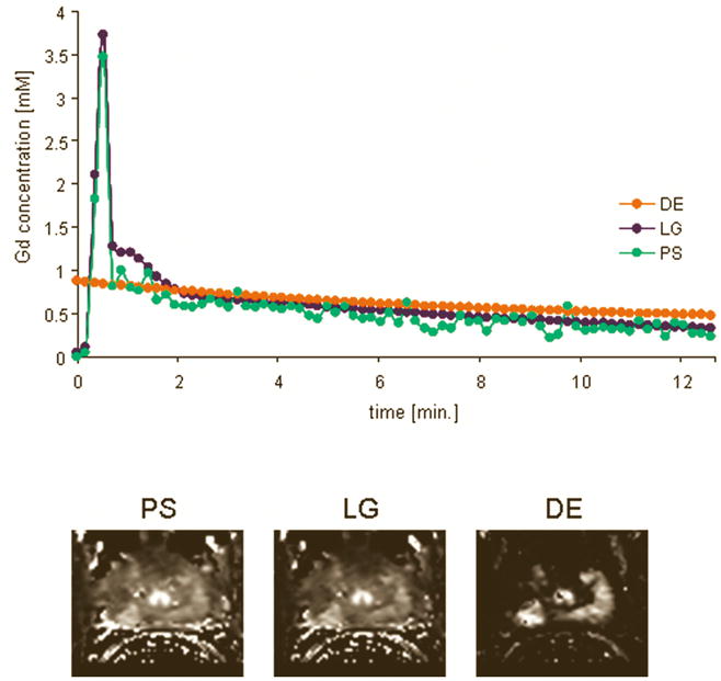
Top: Three AIFs from a 62 years old patient with biopsy proven carcinoma in right apex. Bottom: K^trans parametric maps calculated with the 3 AIFs; all three parametric maps show increased K^trans values in the right apex.

Table 2 shows the performance measures for the 3 AIFs. The patient specific and local Gaussian AIFs had the highest sensitivity of 76%, while the double exponential AIF had the highest specificity of 82%.

Table 2.

Performance measures for the 3 AIFs.

	PS	LG	DE
sensitivity	76% (22/29) (68% – 82%)	76% (22/29) (68% – 82%)	65% (19/29) (58% – 73%)
specificity	77% (167/217) (70% – 83%)	76% (164/217) (68% – 82%)	82% (177/217) (75% – 87%)
PPV	31% (22/72) (24% – 38%)	29% (22/75) (23% – 37%)	32% (19/59) (25% – 40%)
NPV	96% (167/174) (91% – 98%)	96% (164/171) (91% – 98%)	95% (177/187) (90% – 97%)
accuracy	77% (189/246) (69% – 83%)	76% (186/246) (69% – 83%)	80% (196/246) (73% – 85%)

PS – patient specific AIF,

LG – average of individual measured AIFs fitted to double Gaussian plus exponential function,

DE – population average double exponential AIF

PPV – positive predictive value

NPV – negative predictive value

95% confidence intervals are provided in brackets

Figure 2 shows ROC curves generated for all 3 AIFs. The areas under the ROC curves (AUC) were: 0.81, 0.76, and 0.81 for the PS, LG, and the DE AIFs respectively. There were no statistically significant differences in the AUC between any of the AIFs.

Figure 2.

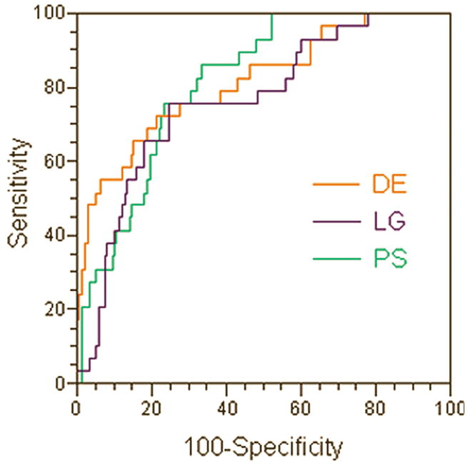
ROC curves generated for the 3 AIFs. The areas under the ROC curves (AUC) were: 0.81, 0.76, and 0.81 for the patient specific (PS), Gaussian local population average (LG), and the double exponential population average (DE) AIFs respectively. There were no statistically significant differences in the AUC between any of the AIFs.

Table 3 shows the median values of the goodness of fit (χ²) for the 3 AIFs. The χ² analyses were carried out in four groups: true positives, i.e. the enhancing regions with positive biopsy, false positives, i.e. enhancing regions with negative biopsies, true negatives, i.e. non-enhancing regions with negative biopsies, and false negatives, i.e. non-enhancing regions with positive biopsies. The Mann-Whitney test results showed that χ² was not significantly different between the 3 AIFs, in all four categories. However, the enhancing regions (both true and false positives) had significantly higher χ² value than the non-enhancing regions (both true and false negatives) for all 3 AIFs.

Table 3.

The median values of the goodness of fit (χ²) for the 3 AIFs.

	PS	LG	DE
TP	0.2962 (0.1070 – 0.9060)	0.2470 (0.0795 – 0.7537)	0.2493 (0.0903 – 1.4474)
TN	0.1764 (0.0390 – 1.2353)	0.1609 (0.0391 – 1.2426)	0.1539 (0.0337 – 1.2359)
FP	0.2106 (0.0832 – 0.9487)	0.2216 (0.0562 – 0.9952)	0.1823 (0.0395 – 1.0267)
FN	0.1073 (0.0691 – 0.2736)	0.0750 (0.0529 – 0.1361)	0.0753 (0.0367 – 0.5300)

TP – true positives (enhancing regions with positive biopsy)

TN – true negatives (non-enhancing regions with negative biopsies)

FP – false positives (enhancing regions with negative biopsies)

FN – false negatives (non-enhancing regions with positive biopsies)

PS – patient specific AIF

LG – average of individual measured AIFs fitted to double Gaussian plus exponential function

DE – population average double exponential AIF

Discussion

As expected, fitting the DCE MRI data with all 3 AIFs resulted in significantly higher K^trans values in prostatic carcinoma (PCa) than in normal peripheral zone (PZ). Such increase in K^trans values has been commonly seen in prostate cancers, and can be explained by increased permeability of the fast growing micro-vessels and the generally higher blood flow in prostate tumours [26]. Differences in K^trans values between the PS and LG vs. DE are most likely related to the differences in the peak amplitude in the three AIFs. DE AIF had the lowest peak amplitude (see Figure 1) and the highest average K^trans value (see Table 1). Perhaps then the accurate measurement of the peak amplitude of the AIF, although it certainly influences the accuracy of the K^trans measurement, may have less significant impact on distinguishing between PCa and normal PZ, which is supported by the results of the ROC analysis in our study.

It is somewhat surprising that the results of fitting with population average AIFs, both DE and LG, also showed significantly smaller values of v_p in PCa, as compared to normal PZ. Since v_p represents the fractional blood volume in the Kety model, one would expect v_p to be higher in PCa than in normal prostatic tissue. This discrepancy may likely be explained by the lower accuracy of fitting the DCE data into the extended Kety model in the fast enhancing regions. This is especially the case when the relatively low temporal resolution of the DCE data prevents accurate sampling of the very fast initial image intensity enhancement, which was the case in this study. This is also supported by the fact that in the logistic regression model built on all 3 DCE MRI parameters (data not shown), v_p did not significantly contribute to the model, thus suggesting that v_p and K^trans were not independent parameters.

The PS and LG AIFs had higher sensitivity in predicting the biopsy results than the DE AIF (76% for PS and LG vs. 65% for DE), though the DE AIF had the highest specificity (82% for DE vs. 77% for PS and 76% for LG). However, the 95% confidence intervals overlap suggests that these differences are not statistically significant. Receiver Operating Characteristic (ROC) analysis showed that the areas under the ROC curves (AUC) were statistically significant (i.e. AUC was significantly higher than 0.5, p = 0.0001) for all 3 AIFs. The PS and DE had higher AUC values than LG (0.81 for PS and DE vs. 0.76 for LG); however these differences were not statistically significant. This result suggests that all three AIFs are equally accurate in predicting the biopsy results in prostate cancer in this study.

There has been little research directed to comparing different models of the AIF. McGrath et al. [27] compared the accuracy of the output parameters of pharmacokinetic model for four forms of AIF, including the bi-exponential, modified bi-exponential, double Gaussian model and simplified Gaussian AIFs. However, this work was carried out in an animal model and did not address the influence of the AIF on diagnostic capabilities of the DCE MRI technique. Although high temporal resolution has been achieved in a number of settings, many recent clinical studies in DCE MRI of prostate cancer still suffer from low temporal resolution [28–30], due to requirements for signal-to-noise ratio, resolution, and anatomic coverage. As a result, assumed models have been commonly used considering the AIF measurements acquired at low temporal resolution could have been unreliable [30]. Our study addressed the issue of whether using measured AIF would provide more accurate diagnosis than using the bi-exponential model.

Goodness of fit (χ²) analysis clearly shows that the quality of fit is higher in the non-enhancing regions than in the enhancing regions (see Table 3). This is most likely the result of inaccuracy of estimating the true AIF. The shape of the DE AIF clearly differs from the shape of the AIF measured experimentally, both in our study and those previously reported [19]. Although the shapes of the PS and LG AIFs estimate more accurately the expected true shape of the AIF, the relatively low temporal resolution used in this study results in inaccurate measurement of the peak amplitude, which in turn results in poorer fit. It is surprising, however, that there were no significant differences in χ² between the PS and LG AIFs and the DE AIF, considering the shape of the PS and LG being more accurate and the peak amplitude being closer to the true value than for the DE. Perhaps the reason is that χ² reflects the goodness of fit for all time points, and the peak amplitude will influence only initial points during fast enhancement, thus having relatively small effect on the overall goodness of fit.

Local population average AIF (i.e. LG) did not perform better than the individually measured PS AIF. This is not unexpected, as in this study we processed only data from patients from whom the AIF could be reliably measured. However, considering that LG performed as well as PS – they both had the same sensitivity and the difference in AUC was not significant, our results suggest that indeed a local population averaged AIF may be of use in processing data from patients for whom the AIF cannot be measured experimentally. It is likely that this would still be the case when high temporal resolution can be used to acquire the DCE MRI data.

A limitation of this study is that the biopsy rather then histology of the prostatectomy specimens was used to validate the presence of tumours. As a result the study concentrated on detecting tumours in the peripheral zone. Since 70% of prostate tumours are located in the peripheral zone and only 5% – 10% of patients will have cancer in the transitional zone and no cancer in the peripheral zone, the standard biopsy protocol does not include the transitional zone. However, since all 3 AIFs were correlated with biopsy, it is not clear whether this had a significant effect on the results and conclusions from the study. The K^trans maps generated with the 3 AIFs showed different size of hyperintense areas (i.e. tumours – see Figure 1), thus having the histology sections of the prostatectomy specimens would allow to compare which AIF gives the best estimate of the tumour volume, which was not possible in this study.

In conclusion, the results of our study suggest that, when limited temporal resolution is used to acquire DCE MRI data, experimentally measured individual Arterial Input Function is not significantly better than population average AIF in predicting the biopsy results in prostate cancer.

References

- 1.Hricak H, Dooms GC, Jeffrey RB, et al. Prostatic carcinoma: Staging by clinnical assesment, CT and MR imaging. Radiology. 1987;162:331–336. doi: 10.1148/radiology.162.2.3797645. [DOI] [PubMed] [Google Scholar]
- 2.Barentsz JO, Engelbrecht M, Jager GJ, et al. Fast dynamic gadolinium-enhanced MR imaging of urinary bladder and prostate cancer. J Magn Reson Imaging. 1999;10:295–304. doi: 10.1002/(sici)1522-2586(199909)10:3<295::aid-jmri10>3.0.co;2-z. [DOI] [PubMed] [Google Scholar]
- 3.Buckley DL, Roberts C, Parker GJ, et al. Prostate cancer: evaluation of vascular characteristics with dynamic contrast-enhanced T1-weighted MR imaging--initial experience. Radiology. 2004;233:709–715. doi: 10.1148/radiol.2333032098. [DOI] [PubMed] [Google Scholar]
- 4.Padhani AR, MacVicar AD, Gapinski CJ, et al. Effects of androgen deprivation on prostatic morphology and vascular permeability evaluated with mr imaging. Radiology. 2001;218:265–374. doi: 10.1148/radiology.218.2.r01ja04365. [DOI] [PubMed] [Google Scholar]
- 5.Engelbrecht MR, Huisman HJ, Laheij RJ, et al. Discrimination of prostate cancer from normal peripheral zone and central gland tissue by using dynamic contrast-enhanced MR imaging. Radiology. 2003;229:248–254. doi: 10.1148/radiol.2291020200. [DOI] [PubMed] [Google Scholar]
- 6.Jager GJ, Ruijter ET, van de Kaa CA, et al. Dynamic TurboFLASH subtraction technique for contrast-enhanced MR imaging of the prostate: correlation with histopathologic results. Radiology. 1997;203:645–652. doi: 10.1148/radiology.203.3.9169683. [DOI] [PubMed] [Google Scholar]
- 7.Padhani AR, Gapinski CJ, Macvicar DA, et al. Dynamic contrast enhanced MRI of prostate cancer: correlation with morphology and tumour stage, histological grade and PSA. Clin Radiol. 2000;55:99–109. doi: 10.1053/crad.1999.0327. [DOI] [PubMed] [Google Scholar]
- 8.Noworolski SM, Henry RG, Vigneron DB, et al. Dynamic contrast-enhanced MRI in normal and abnormal prostate tissues as defined by biopsy, MRI, and 3D MRSI. Magn Reson Med. 2005;53:249–255. doi: 10.1002/mrm.20374. [DOI] [PubMed] [Google Scholar]
- 9.Muramoto S, Uematsu H, Kimura H, et al. Differentiation of prostate cancer from benign prostate hypertrophy using dual-echo dynamic contrast MR imaging. Eur J Radiol. 2002;44:52–58. doi: 10.1016/s0720-048x(01)00468-5. [DOI] [PubMed] [Google Scholar]
- 10.Choyke PL, Dwyer AJ, Knopp MV. Functional tumor imaging with dynamic contrast-enhanced magnetic resonance imaging. J Magn Reson Imaging. 2003;17:509–520. doi: 10.1002/jmri.10304. [DOI] [PubMed] [Google Scholar]
- 11.Brawer MK, Deering RE, Brown M, et al. Predictors of pathologic stage in prostatic carcinoma. The role of neovascularity. Cancer. 1994;73:678–687. doi: 10.1002/1097-0142(19940201)73:3<678::aid-cncr2820730329>3.0.co;2-6. [DOI] [PubMed] [Google Scholar]
- 12.Bostwick DG, Wheeler TM, Blute M, et al. Optimized microvessel density analysis improves prediction of cancer stage from prostate needle biopsies. Urology. 1996;48:47–57. doi: 10.1016/s0090-4295(96)00149-5. [DOI] [PubMed] [Google Scholar]
- 13.Rijpkema M, Kaanders JH, Joosten FB, et al. Method for quantitative mapping of dynamic MRI contrast agent uptake in human tumors. J Magn Reson Imaging. 2001;14:457–463. doi: 10.1002/jmri.1207. [DOI] [PubMed] [Google Scholar]
- 14.Hawighorst H, Knapstein PG, Weikel W, et al. Angiogenesis of uterine cervical carcinoma: characterization by pharmacokinetic magnetic resonance parameters and histological microvessel density with correlation to lymphatic involvement. Cancer Res. 1997;57:4777–4786. [PubMed] [Google Scholar]
- 15.Hawighorst H, Knopp MV, Debus J, et al. Pharmacokinetic MRI for assessment of malignant glioma response to stereotactic radiotherapy: initial results. J Magn Reson Imaging. 1998;8:783–788. doi: 10.1002/jmri.1880080406. [DOI] [PubMed] [Google Scholar]
- 16.Evelhoch JL. Key factors in the acquisition of contrast kinetic data for oncology. J Magn Reson Imaging. 1999;10:254–259. doi: 10.1002/(sici)1522-2586(199909)10:3<254::aid-jmri5>3.0.co;2-9. [DOI] [PubMed] [Google Scholar]
- 17.Parker GJ, Padhani AR. T1-weighted dynamic contrast enhanced MRI. In: Tofts PS, editor. Quantitative MRI of the brain-measuring changes caused by disease. Chichester: John Wiley and Sons Ltd; 2003. pp. 341–364. [Google Scholar]
- 18.Tofts PS, Berkowitz B, Schnall MD. Quantitative analysis of dynamic Gd-DTPA enhancement in breast tumors using a permeability model. Magn Reson Med. 1995;33:564–568. doi: 10.1002/mrm.1910330416. [DOI] [PubMed] [Google Scholar]
- 19.Parker GJ, Roberts C, Macdonald A, et al. Experimentally-derived functional form for a population-averaged high-temporal-resolution arterial input function for dynamic contrast-enhanced MRI. Magn Reson Med. 2006;56:993–1000. doi: 10.1002/mrm.21066. [DOI] [PubMed] [Google Scholar]
- 20.Parker GJ, Suckling J, Tanner SF, et al. Probing tumor microvascularity by measurement, analysis and display of contrast agent uptake kinetics. J Magn Reson Imaging. 1997;7:564–574. doi: 10.1002/jmri.1880070318. [DOI] [PubMed] [Google Scholar]
- 21.Tofts PS, Brix G, Buckley DL, et al. Estimating kinetic parameters from dynamic contrast-enhanced T(1)-weighted MRI of a diffusable tracer: standardized quantities and symbols. J Magn Reson Imaging. 1999;10:223–232. doi: 10.1002/(sici)1522-2586(199909)10:3<223::aid-jmri2>3.0.co;2-s. [DOI] [PubMed] [Google Scholar]
- 22.Kozlowski P, Chang SD, Jones EC, et al. Combined diffusion-weighted and dynamic contrast-enhanced MRI for prostate cancer diagnosis - correlation with biopsy and histopathology. J Magn Reson Imaging. 2006;24:108–113. doi: 10.1002/jmri.20626. [DOI] [PubMed] [Google Scholar]
- 23.Mould RF. Introductory Medical Statistics. Bristol and Philadelphia: Institute of Physics Publishing; 1998. Sensitivity and Specificity; pp. 232–233. [Google Scholar]
- 24.Newcombe RG. Two-sided confidence intervals for the single proportion: comparison of seven methods. Stat Med. 2008;17:857–872. doi: 10.1002/(sici)1097-0258(19980430)17:8<857::aid-sim777>3.0.co;2-e. [DOI] [PubMed] [Google Scholar]
- 25.DeLong ER, DeLong DM, Clarke-Pearson DL. Comparing the areas under two ormore correlated Receiver Operating Characteristics curves: A nonparametric approach. Biometrics. 1988;44:837–845. [PubMed] [Google Scholar]
- 26.Inaba T. Quantitative measurements of prostatic blood flow and blood volume by positron emission tomography. J Urol. 1992;148:1457–1460. doi: 10.1016/s0022-5347(17)36939-2. [DOI] [PubMed] [Google Scholar]
- 27.McGrath DM, Bradley DP, Tessier JL, et al. Comparison of model-based arterial input functions for dynamic contrast-enhanced MRI in tumor bearing rats. Magn Reson Med. 2009;61:1173–1184. doi: 10.1002/mrm.21959. [DOI] [PubMed] [Google Scholar]
- 28.Haider MA, Chung P, Sweet J, et al. Dynamic contrast-enhanced magnetic resonance imaging for localization of recurrent prostate cancer after external beam radiotherapy. Int J Radiat Oncol Biol Phys. 2008;70:425–430. doi: 10.1016/j.ijrobp.2007.06.029. [DOI] [PubMed] [Google Scholar]
- 29.Hara N, Okuizumi M, Koike H, et al. Dynamic contrast-enhanced magnetic resonance imaging (DCE-MRI) is a useful modality for the precise detection and staging of early prostate cancer. Prostate. 2005;62:140–147. doi: 10.1002/pros.20124. [DOI] [PubMed] [Google Scholar]
- 30.Langer DL, van der Kwast TH, Evans AJ, et al. Prostate cancer detection with multi-parametric MRI: logistic regression analysis of quantitative T2, diffusion-weighted imaging, and dynamic contrast-enhanced MRI. J Magn Reson Imaging. 2009;30:327–334. doi: 10.1002/jmri.21824. [DOI] [PubMed] [Google Scholar]