EXTRACTING PRINCIPLE COMPONENTS FOR DISCRIMINANT ANALYSIS OF FMRI IMAGES

Abstract

This paper presents an approach for selecting optimal components for discriminant analysis. Such an approach is useful when further detailed analyses for discrimination or characterization requires dimensionality reduction. Our approach can accommodate a categorical variable such as diagnosis (e.g. schizophrenic patient or healthy control), or a continuous variable like severity of the disorder. This information is utilized as a reference for measuring a component’s discriminant power after principle component decomposition. After sorting each component according to its discriminant power, we extract the best components for discriminant analysis. An application of our reference selection approach is shown using a functional magnetic resonance imaging data set in which the sample size is much less than the dimensionality. The results show that the reference selection approach provides an improved discriminant component set as compared to other approaches. Our approach is general and provides a solid foundation for further discrimination and classification studies.

1. INTRODUCTION

Neuroimaging techniques, such as magnetic resonance imaging (MRI) and positron emission tomography, have been utilized both in research and clinic fields, to scan brain structure or function for diagnosis and/or prognosis of mental disorders. There is growing interest in incorporating genetic information and brain images to study the genetic influence of an inherited mental disorder [1]. Brain imaging data often contains hundreds of thousands of voxels that need to be analyzed. Similarly, the amount of genes or single nucleotide polymorphisms is typically large too. It is desirable to extract features or components from the high dimensional data which convey useful information.

Principle component analysis (PCA) has been used for data reduction, component selection, and also considered for linear discriminate analysis [2–4]. It can be described in a generic form as S=W·X, where S are the extracted components, X are the original measurements, and W is the projection matrix. It is well known that the best components for discrimination are not necessarily those with the largest variance. A measure of the component importance from discriminant perspective was introduced by Chang [3], and further developed by Dillon et. al. [4] and Jolliffe et. al. [2]. This measure is essentially a normalized between-group difference after projecting to each component’s direction. These measures were developed for datasets which have a larger sample size than the dimensionality.

However, there are two limitations about the between-group difference measure proposed by Chang, when applied to brain image analysis or genetic data. One is related to the sample size and the dimensionality of the data. For functional MRI (fMRI) data, we consider a group analysis in which the dimensionality is the number of voxels, which is much larger than the number of subjects. Activation in each voxel of a brain image is of interest for a specific task. As exemplified in a feature-based classification application [5], where brain activation images were used, X is arranged as a subjects-by-voxels matrix, S is a components-by-voxels matrix, and voxels ≫ subjects. In such a case, due to limited computational resources, the between-group difference measure is not tractable without an extra modification which will be explained in detail in the methods section.

The other limitation is that the between-group differences are defined only for categorical factors. In practice, additional non-categorical information, beyond group membership, such as age, race, severity of the disorder, etc., all can potentially be discriminant factors. Many of them are the focuses of biomedical researches. Therefore, a new approach is needed for the selection of components to discriminate certain groups according to different factors from a population using their fMRI brain images.

In this paper we provide a systemic approach to select the best components for discrimination, with a flexible setting. We first introduce the method in section 2 and then explore its application to fMRI data in section 3. Results are presented in Section 4, followed by discussion and conclusion.

2. METHODS

2.1. PCA dimensionality reduction using variance

PCA is mathematically defined to transform data into a new orthogonal coordinate system, such that the greatest variance of data is captured by the first coordinate, the second greatest variance by the second coordinate, and so on. Consider X, an N-by-D matrix, to be zero mean observations collected from groups of subjects, N is the subjects’ number and D is the number of dimensions (N≪D for our applications). Components of interest here are the patterns embedded in the data among all the subjects, which remove the duplicated information among subjects and preserves the distinct patterns only. To do so, PCA is employed as described by (1), where C_X is an N-by-N covariance matrix, W is an N-by-N eigenvector matrix of the covariance matrix and Λ is the corresponding N-by-N eigenvalue matrix. In a typical use of principle component for dimensionality reduction, the top M components (M<N) with the largest eigenvalues (e.g. carrying the most variance) are selected. The W matrix is then reduced to Ŵ, an N-by-M matrix, and S is reduced from an N-by-D component matrix to an M-by-D component matrix Ŝ.

$$\begin{array}{l}{C}_X=E\{X·X^T\};C_X·W=W·\mathrm{\Lambda };\\ S=W^T·X;\widehat{S}={\widehat{W}}^T·X;\end{array}$$ (1)

2.2. Between-group difference selection of component

Since the components carrying the most variance may not be the ones best characterizing group differences, variance is not the ideal criterion for selecting the best components for discriminant analysis. An alternative score, θ, is defined as a selection criteria in (2) by Chang [3]. The vector d is the mean difference vector between the respective groups. For this case, d is consisted of D elements. Similarly, w̃_i is the i^th eigenvector with D elements instead of N elements, computed through the covariance matrix C̃_X (a D-by-D matrix). λ̃_i is the corresponding i^th eigenvalue. The score represents the actual between-group mean difference projected into each eigenvector direction, and normalized by the component’s variance. For brain images or genetic data, the dimension of D is easily over tens of thousands. Computing the covariance matrix C̃_X and its eigenvectors can be intractable for regular computers due to the large amount of memory required. To avoid the computational difficulty of computing such a large covariance matrix, a substitute approach is proposed in (3) to identify N valid eigenvectors [6]. Then, the N θ scores can be calculated and sorted in a descending order. The top M eigenvectors w̃ are then identified from the top M θ scores, as well as their paired eigenvectors W. Components are selected accordingly by projecting X into the M eigenvectors of W.

$$\begin{array}{l}{\stackrel{\sim }{C}}_X=E\{X^T·X\};{\stackrel{\sim }{C}}_X·\stackrel{\sim }{W}=\stackrel{\sim }{W}·\stackrel{\sim }{\mathrm{\Lambda }};\\ {\theta }_i=\frac{{({\stackrel{\sim }{w}}_i^{T}d)}^2}{{\stackrel{\sim }{\lambda }}_i}\end{array}$$ (2)

$$\begin{array}{l}(X·X^T)·W=W·\mathrm{\Lambda };\\ \stackrel{\sim }{W}=X^T·W·{\mathrm{\Lambda }}^{-1/2};\end{array}$$ (3)

2.3. Reference selection of component

In this section, we propose a new approach for selecting the optimal components for discrimination based on a reference. The reference vector is first defined according to the subjects’ information. For the simplest case, there are two groups: one group of N₁ patients and one group of N₂ healthy controls (N=N₁+N₂). If group membership is the discriminant criterion, the reference vector can be constructed as a column vector consisting of −1/N₁ (N1 times) and 1/N₂ (N2 times), with a sum of zero, and assigning equal weight to each group. A new score ϕ, is proposed in (4) as a measure of discriminant power via the reference. In this equation, r is the reference vector that encodes subjects’ group information, λ_i is the i^th eigenvalue and w_i is the corresponding i^th eigenvector. Thus, using the above case, the score function for each component becomes Equation (5), projecting the eigenvector into the reference direction, scaled by the eigenvalue.

After sorting the ϕ values in a descending order, as well as the corresponding eigenvectors, the top M components are selected for discriminant purpose by projecting X into the top M eigenvectors.

$$\begin{array}{l}\varphi =\mid \mathrm{\Lambda }·(W^T·r)\mid ;\mathit{Then},{\varphi }_i=\mid {\lambda }_i·w_i^T·r\mid ;\\ \widehat{S}={\widehat{W}}^T·X;\end{array}$$ (4)

$${\varphi }_i=\mid {\lambda }_i·w_i^T·{[\underset{N_1}{\underbrace{\frac{-1}{N_1},\frac{-1}{N_1},\dots ,\frac{-1}{N_1},}}\underset{N_2}{\underbrace{\frac{1}{N_2},\frac{1}{N_2},\dots ,\frac{1}{N_2}}}]}^T\mid ;$$ (5)

Since W is the orthogonal eigenvector matrix, we can use this orthogonality to derive Equation (6).

$$W^{-1}=W^T;X=W·S;$$ (6)

Each column of W is an eigenvector containing the loading parameters of each component.

Thus, the score function can be interpreted as the correlation of the loading parameters of the component with the reference, scaled with the corresponding variance. In the above example, the correlation of the loading parameter with the reference is, in fact, the mean difference of the loading parameters between two groups. The score ϕ indicates the component’s variance showing the group difference of the loading parameters.

The reference vector can be very flexible, varying with the desired information of interest. For example, if we are interested in the severity of schizophrenic disorder, the reference can be a continuous number vector of positive and negative syndrome scale scores, indicating different levels of severity.

2.4 Evaluation method

To evaluate the results of difference approaches, a two-sample t-test on the loading parameters (i.e. eigenvector elements) of selected components is performed. We also want to test the improvement of the ultimate performance (outcome of further study on the components) using the selected components. As an example, brain networks extracted from components selected by three approaches are compared.

3. APPLICATION

FMRI has been frequently utilized as a noninvasive tool for studying schizophrenia. Extracting characteristic features to identify the patients helps further understanding and treatment of the disorder. We demonstrate feature selection approaches for fMRI components in the paper. Data from 30 schizophrenia patients and 30 healthy controls were included. All of them provided written, informed, IRB-approved consent at Hartford Hospital.

FMRI data were acquired during an auditory oddball (AOD) task at the Olin Neuropsychiatry Research Center at the Institute of Living. The AOD task involves detecting an infrequent sound (the target) within a series of frequent sounds. A full description of task design is available in reference [7]. The participants were instructed to respond as quickly and accurately as possible with their right index finger every time they heard a target stimulus. FMRI scans were acquired on a Siemens Allegra 3T dedicated head MRI scanner. FMRI images were preprocessed, including realignment, normalization and smoothing, using the software package SPM2 (http://www.fil.ion.ucl.ac.uk/spm/). Target-related contrast images (77026 voxels of interest) were used in this study.

The component number is estimated via a modified Akaike’s Information Criterion [8]. The top four out of a possible 60 components from each approach are assigned to represent the discriminant information for the fMRI data.

4. RESULTS

Components selected by variance, group membership reference (a vector constructed with 1/30, and −1/30) and between-group difference are presented here. Table 1 shows two-sample t-test results (patients versus controls) for each component selected by each approach. With a p-value threshold of 0.05, bold components in the table indicate the ones with significant group differences (p<0.05). Two components are identified in the results of variance selection, and two in the results of between-group difference selection. Our approach, reference selection, found three components with significant group differences.

Table 1.

Two-sample t-test for selected components

	value	Com. 1*	Com. 2	Com. 3	Com. 4
Variance selection	P	0.0099	0.0001	0.3222	0.6827
	T	2.6736	−4.1940	−1.0032	−0.4110
Difference selection	P	0.0001	0.0083	0.0742	0.0994
	T	−4.1940	2.7716	1.8196	−1.6873
Reference selection	P	0.0099	0.0001	0.0083	0.3222
	T	2.6736	−4.1940	2.7716	−1.0032

^*Com.# indicates the #^th component.

In addition, we computed a two-sample t-test on all possible 60 components, and found that only 3 components show significant group differences. All three components were in fact selected by the reference approach, plotted in Fig. 1(A–C). For display, components were plotted only in voxels with an absolute activation Z score larger than 2. Red color indicates positive activations, and blue color indicates negative activations. Components A and B in Fig. 1 were selected by the variance approach, and components B and C were selected by the between-group difference approach.

Figure 1.

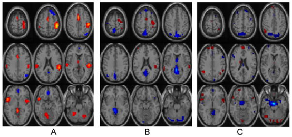
Significant components

Component A in Fig. 1 shows activations mainly in superior temporal gyrus, cingulate gyrus, and medial frontal gyrus. These locations are well-known to be activated during an auditory task, and present discriminant properties for schizophrenia patients [9]. Component B includes posterior cingulate gyrus and superior frontal gyrus, which are often studied for schizophrenic disorder. Component C shows activations mainly in precuneus and uncus that is partially consistent with our previous finding [1].

5. DISCUSSION AND CONCLUSION

The components selected using variance present the major activation regions during the AOD task, including bilateral superior temporal gyri, prefrontal gyrus, cingulate cortex and thalamus. However, only two out of four components show significant group differences. Considering the components selected by the reference approach, one component is different from those selected by variance, and that is the additional one showing group difference in the t-test. Therefore, the reference approach selects a complete set of discriminant components, and at the same time captures as more variance as possible.

Two components from the between-group difference selection show group differences, and the other two components are different from those selected by variance (and do show larger group differences, albeit not significant). The reason for that is because the score θ is normalized by variance, such that the order of variance not represented in the selected components. Moreover, the modification of between-group difference selection in (3), has to be executed, which results in more calculations, and may affect the order of the components. More investigation is needed.

It is evident that the reference selection extracted more discriminate components than the other two approaches. These components will then contribute to further discriminate analysis. For example, independent component analysis has been utilized for the study of fMRI data [10, 11], where principle components serve as input features for finding independent brain functional networks. If the interest is the distinguishing brain networks between patients and healthy controls, the idea input features are that carrying group difference information. As an example, we applied the components selected by three approaches into ICA, to extract independent brain functional networks that show difference between patients and healthy controls. One brain network indicating group difference was extracted from the results of variance selection, plotted in Fig. 2(a). Three brain networks were extracted from the results of reference selection, plotted in Fig. 2(a,b,c). Three brain networks were also extracted from the results of between-group difference selection, and include similar brain regions as those extracted from reference selection, but are sparser. Based on two-sample t-tests, brain networks from reference selection show lower p-values (average of 0.0028) and higher t-values(average of 3.60) than those from between-group difference selection (average p-value of 0.0038, average t-value of 3.30).

Figure 2.

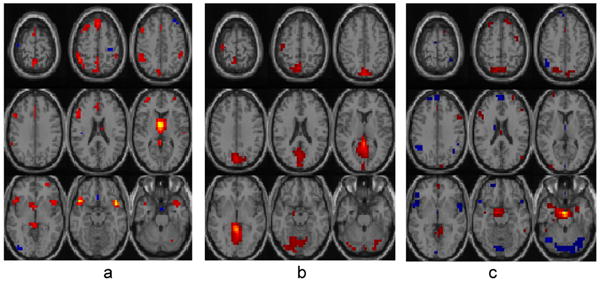
Brain networks indicating group differences

In summary, the reference selection approach is straightforward to implement, especially in the biomedical filed where the dimensionality is typically larger than the number of subjects. The reference function in our approach is very flexible, useful under a variety of conditions. Most importantly, this selection approach provides the most complete discriminate component set compared with the other two approaches. It can then be useful for further analyzing, understanding, and characterizing the distinctions among groups.

References

- 1.Liu J, Pearlson G, Windemuthe A, Ruaño G, Perrone-Bizzozerof NI, Calhoun V. Combining fMRI and SNP data to investigate connections between brain function and genetics using parallel ICA. Human Brain Mapping. 2007 doi: 10.1002/hbm.20508. In press. [DOI] [PMC free article] [PubMed] [Google Scholar]
- 2.Jolliffe IT, Morgan BJT, Young PJ. A simulation study of the use of principle component in linear discriminat analysis. Journal of statistical computation and simulation. 1996;55:353–366. [Google Scholar]
- 3.Chang WC. on using principle components before separating a mixture of two multivariate normal distributions. applied statistics. 1983;32:267–275. [Google Scholar]
- 4.Dillon RW, Mulani N, Frederick GD. On the use of component scores in the presence of group structure. Journal of consumer research. 1989;16:106–112. [Google Scholar]
- 5.Calhoun V, Adali T, Liu J. A Feature-Based Approach to Combine Functional MRI, Structural MRI and EEG Brain Imaging Data. Engineering in Medicine and Biology Society, 2006. EMBS ’06. 28th Annual International Conference of the IEEE; New York, NY. Aug. 2006; pp. 3672–3675. [DOI] [PubMed] [Google Scholar]
- 6.Wall EM, Rechtsteiner A, Rocha ML. Singular value decomposition and principal component analysis. In: Berrar PD, Dubitzky W, Granzow M, editors. A Practical Approach to Microarray Data Analysis. Kluwer; Norwell, MA: 2003. pp. 91–109. [Google Scholar]
- 7.Kiehl KA, Stevens MC, Laurens KR, Pearlson G, Calhoun VD, Liddle PF. An adaptive reflexive processing model of neurocognitive function: supporting evidence from a large scale (n = 100) fMRI study of an auditory oddball task. Neuroimage. 2005 Apr 15;25:899–915. doi: 10.1016/j.neuroimage.2004.12.035. [DOI] [PubMed] [Google Scholar]
- 8.Li YO, Adali T, Calhoun VD. Estimating the number of independent components for functional magnetic resonance imaging data. Hum Brain Mapp. 2007 Feb 1; doi: 10.1002/hbm.20359. [DOI] [PMC free article] [PubMed] [Google Scholar]
- 9.Kiehl KA, Liddle PF. An event-related functional magnetic resonance imaging study of an auditory oddball task in schizophrenia. Schizophr Res. 2001 Mar;48:159–71. doi: 10.1016/s0920-9964(00)00117-1. [DOI] [PubMed] [Google Scholar]
- 10.Calhoun VD, Adali T. Unmixing fMRI with independent component analysis. IEEE Eng Med Biol Mag. 2006 Mar–Apr;25:79–90. doi: 10.1109/memb.2006.1607672. [DOI] [PubMed] [Google Scholar]
- 11.Liu J, Calhoun V. Parallel independent component analysis for multimodal analysis: application to fmri and eeg data. Biomedical Imaging: From Nano to Macro, 2007. ISBI 2007. 4th IEEE International Symposium; Apr 2007.pp. 1028–1031. [Google Scholar]