

Abstract
Independent component analysis (ICA) utilizing prior information, also called semiblind ICA, has demonstrated considerable promise in the analysis of functional magnetic resonance imaging (fMRI). So far, temporal information about fMRI has been used in temporal ICA or spatial ICA as additional constraints to improve estimation of task‐related components. Considering that prior information about spatial patterns is also available, a semiblind spatial ICA algorithm utilizing the spatial information was proposed within the framework of constrained ICA with fixed‐point learning. The proposed approach was first tested with synthetic fMRI‐like data, and then was applied to real fMRI data from 11 subjects performing a visuomotor task. Three components of interest including two task‐related components and the “default mode” component were automatically extracted, and atlas‐defined masks were used as the spatial constraints. The default mode network, a set of regions that appear correlated in particular in the absence of tasks or external stimuli and is of increasing interest in fMRI studies, was found to be greatly improved when incorporating spatial prior information. Results from simulation and real fMRI data demonstrate that the proposed algorithm can improve ICA performance compared to a different semiblind ICA algorithm and a standard blind ICA algorithm. Hum Brain Mapp, 2010. © 2009 Wiley‐Liss, Inc.
Keywords: fMRI analysis, spatial ICA, semiblind ICA, constrained ICA, spatial constraints, fixed‐point learning
INTRODUCTION
Independent component analysis (ICA) consists of recovering a set of maximally independent sources from their observed mixtures without knowledge of the source signals and the mixing parameters [Cardoso,1998; Cichocki and Amari,2003; Hyvärinen et al.,2001]. Functional magnetic resonance imaging (fMRI) is a widely used brain imaging technique which is based upon the hemodynamic response resulting from neuronal activity. Since the hemodynamic response and its connection to neuronal activity are not fully understood, ICA has become a useful approach for identifying either spatially independent components (spatial ICA) or temporally independent components (temporal ICA) from fMRI data [Calhoun and Adali,2006; De Martino et al.,2007; Mckeown et al.,1998].
In practice, spatial or temporal information about fMRI data is often available to provide additional constraints on the estimation of the sources or the mixing matrix. For example, the default mode network (a set of regions that appear correlated in particular in the absence of tasks or external stimuli) is of great interest [Beckmann et al.,2005; Calhoun et al.,2008a; Garrity et al.,2007; Greicius et al.,2003; McKiernan et al.,2003; Raichle et al.,2001], and its spatial pattern has been consistently identified in multiple papers [Beckmann et al.,2005; Biswal and Ulmer,1999; Cordes et al.,2000; Damoiseaux et al.,2006; Garrity et al.,2007]. In addition, temporal information about the brain activation model for fMRI is also available [Calhoun et al.,2005; Lu and Rajapakse,2005]. Recent work has suggested that incorporating prior information into the estimation process, also called semiblind ICA, can improve the potential of ICA as a method for fMRI analysis [Calhoun et al.,2005; Lu and Rajapakse,2005].
Depending upon which type of independence is assumed and what constraints are used, semiblind ICA algorithms can be classified into four categories: (1) Temporal semiblind temporal ICA, in which temporal independence is assumed and temporal constraints on the sources are used. The ICA with reference (ICA‐R) algorithm proposed by Lu and Rajapakse is such an algorithm [Lu and Rajapakse,2005]. (2) Spatial semiblind temporal ICA, in which temporal independence is assumed and spatial constraints on the mixing matrix are incorporated. The semiblind source separation algorithm proposed by Hesse and James [Hesse and James,2006] can be used for this purpose. (3) Temporal semiblind spatial ICA, in which spatial independence is assumed and temporal constraints on the mixing matrix are used. The semiblind ICA algorithm proposed by Calhoun et al. belongs to this category [Calhoun et al.,2005]. (4) Spatial semiblind spatial ICA, in which spatial independence is assumed and spatial constraints are applied to the sources, has not yet been proposed or applied to fMRI data despite the available spatial information mentioned above. Among the four categories, the spatial semiblind spatial ICA and the temporal semiblind temporal ICA are closely related, e.g., the ICA‐R algorithm, originally proposed for temporal semiblind temporal ICA, can also be used to perform spatial semiblind spatial ICA. However, the ICA‐R algorithm incorporates Newton‐like learning (i.e., uses a Newton optimization method with a learning rate) [Lu and Rajapakse,2005] which has two drawbacks: (1) sensitivity to the learning rate and initialization of the weight vectors; (2) the need for matrix inversion and second derivatives. As such, this article develops an improved semiblind algorithm in this category for analyzing fMRI data and also presents the application of spatial semiblind spatial ICA to fMRI data.
Among various schemes for developing semiblind ICA algorithms, constrained ICA [Lu and Rajapakse,2000] has two attractive advantages: (1) automatic extraction of desired components in a predefined order, and (2) a significant decrease in computational load [Lu and Rajapakse,2003, 2005]. Therefore, the proposed algorithm was developed within the framework of constrained ICA. To utilize spatial constraints but avoid the limitations of Newton‐like learning (e.g., sensitivity to the learning rate and initialization), a new contrast function was introduced, and then optimized according to the Kuhn‐Tucker conditions [Luenberger,1969]. An efficient fixed‐point algorithm was then derived. The main contribution of this paper is that it provides a new way to utilize available spatial information and is the first application of spatial semiblind spatial ICA to fMRI. By utilizing spatial information, the proposed approach enables more robust estimation of consistently identified spatial networks such as the default mode network (for which we don't have temporal priors), which is of increasing interest in fMRI studies and is an important network for schizophrenia [Garrity et al.,2007] and Alzheimer's disease [Greicius et al.,2004]. Our results indicate that, e.g., the default mode network is not detected as accurately for the ICA approaches which do not utilize prior information.
CONSTRAINED ICA
The ICA model, as typically applied to fMRI data, assumes the observed vector x = [x 1,x 2,…x N]T to be a linear mixture of the source vector s = [s 1,s 2,…s M]T (N ≥ M) by an N × M mixing matrix A, i.e., x = As. Standard blind ICA aims to find an M × N unmixing matrix W such that the output vector y = [y 1,y 2,…y M]T = Wx provides estimates of all M source signals. Standard blind ICA has some problems such as output ambiguity [Cardoso,1998; Cichocki and Amari,2003; Hyvärinen et al.,2001] which can be solved by utilizing prior information about the sources or the mixing matrix.
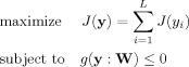
Constrained ICA, proposed by Lu and Rajapakse [Lu and Rajapakse,2000], is a general framework to incorporate available prior information about the sources into standard blind ICA. The prior information is added to the contrast function of a standard blind ICA algorithm in the form of inequality constraints and equality constraints. Specifically, constrained ICA is modeled as the following constrained optimization problem [Lu and Rajapakse,2000, 2005]:
| (1) |
where J(y) denotes the contrast function of a standard blind ICA algorithm,  includes p inequality constraints, and
  includes q equality constraints.
The ICA‐R algorithm is a semiblind algorithm developed in the framework of constrained ICA [Lu and Rajapakse,2005], in which J(y) is the L‐unit contrast function of a standard blind ICA algorithm [Hyvärinen,1998]:
| (2) |
and
| (3) |
where ρ is a positive constant, ν is a Gaussian variable with zero mean and unit variance, and G(·) is a nonquadratic function. The ICA‐R algorithm used L inequality constraints g(y : W) and L equality constraints h(y : W) to constrain J(y) in (1), and then the Lagrange multiplier method was utilized to give a Newton‐like learning algorithm [Lu and Rajapakse,2005].
PROPOSED APPROACH
We aim to provide a spatial semiblind spatial ICA algorithm within the framework of constrained ICA. Assuming the total number of source signals is M, the spatial information about L (1 ≤ L < M, i.e., a subset of all of the sources) sources of interest is available. The proposed approach will automatically extract only the L desired sources from the mixtures in a predefined order instead of estimating all of the M source signals as standard blind ICA usually does. Specifically, L reference signals r 1,…,r L are constructed from the spatial information about the L sources of interest, and a closeness measure ε(y i,r i) between an extracted signal y i and a reference signal r i (i = 1,…,L) is defined to constrain W learning. As a result, only L weight vectors w 1,…, w L (L rows of the unmixing matrix W) will be found to give y 1,…,y L (i.e., y i = w i x), the order of which is the same as that of r 1,…,r L.
The proposed algorithm is specifically formulated in the framework of constrained ICA as follows
 |
(4) |
where  includes L inequality constraints for incorporating spatial information,
  , and ξi is a threshold distinguishing one desired output y
i from the others.
, and ξi is a threshold distinguishing one desired output y
i from the others.
Compared with the model (1) of constrained ICA, we omitted the equality constraint h(y : W) which is included to ensure the contrast function J(y) and the weight vector w are bounded, e.g., h(y: W) = E{y2} − 1 = 0 [Lu and Rajapakse,2000, 2005]. Alternatively, we used the following constraint:
| (5) |
where C = E{xx T} is the covariance of the mixed signals x, δij equals 1 when i = j and equals 0 when i ≠ j. After data whitening, we have C = E{xx T} = I and then get a simplified constraint from Eq. (5) as:
| (6) |
Considering Eqs. (4) and (6), we introduce a new contrast function for the proposed approach as follows
| (7) |
where L(W,μ) is an augmented Lagrangian function from Eq. (4) after transforming g(y : W) into equality constraint with slack variables:
| (8) |
μ = [μ1,…,μL]T includes L positive Lagrange multipliers for the constraint g(y : W), γ = [γ1,…,γL]T includes L positive penalty parameters, and F(‖W‖2) is a penalty term corresponding to the constraint in Eq. (6):
| (9) |
where λi (i = 1,…,L) is a positive Lagrangian coefficient.
To avoid the limitations of Newton‐like learning, we find the maximum of Eq. (7) according to the Kuhn‐Tucker conditions as:
| (10) |
Considering Eqs. (8) and (9), we have
| (11) |
where λ = [λ1,…,λL]T, ρ = ±[ρ1,…,ρL]T includes L constants the signs of which are coincident with E{G(y i)} − E{G(νi)}, G′y(Wx), and g′y (y : W) are the first derivatives of G(Wx) and g(y : W) with respect to y, 〈·〉 denotes a diagonal matrix, the diagonal elements of which are given by the vector inside (e.g., λ, ρ, μ).
For simplicity, the effect of λ in Eq. (11) is omitted by scaling ρ and μ on the right side of the equation [Hyvärinen,1997]. Thus a fixed‐point learning algorithm is obtained as follows:
 |
(12) |
where  and
and  denote the scaled ρ and μ, and are learned by the following rules (
 denotes the scaled γ):
| (13) |
At each iteration step, the weight vectors are decorrelated to prevent different components from converging to the same solution [Hyvärinen,1997; Hyvärinen et al.,2001]:
| (14) |
In summary, Eqs. (12)– (14) form the proposed algorithm. Compared with the ICA‐R algorithm with Newton‐like learning, the proposed algorithm has no learning rate. It is also insensitive to initialization of the weight vectors due to fixed‐point learning. Since the equality constraints are omitted, the matrix inversion and the second derivatives are not needed, the computational complexity of the proposed algorithm is largely decreased compared with ICA‐R.
SIMULATION AND RESULTS
To evaluate the performance of the proposed approach through simulations, we used the simulated fMRI‐like dataset including eight sources at http://mlsp.umbc.edu/simulated_fmri_data.html, and replaced the task‐related source with three new source images to mimic three real fMRI components of interest (two task‐related components and one default mode component).
Noiseless and Noisy fMRI‐Like Data
Figure 1 shows the ten fMRI‐like source images (s 1–s 10, 60 × 60, a value of “1” is colored white and a value of “0” is colored black) and the corresponding time courses (tc1–tc10, 100‐point). Specifically, s1 and s2 simulated two task‐related sources, s 3 simulated default mode source, s4 and s8 simulated two transiently task‐related sources, s 5, s 6, s 7, s 9, and s 10 simulated five artifact‐related sources. The time courses tc1 and tc2 were two model time courses generated by convolving a temporal model of the on‐off task with the default SPM canonical hemodynamic response function [available at: http://www.fil.ion.ucl.ac.uk/spm/; Correa et al.,2007] and tc3 simulated the default mode time course. By mixing the 10 source images with the 10 time courses, we obtained a noiseless mixture simulating 100 scans of a single slice of fMRI data. To examine the robustness of the proposed approach, we also added Gaussian noise to the mixture with three levels of SNR (dB), which were 5 dB, 0 dB, and −5 dB, respectively.
Figure 1.
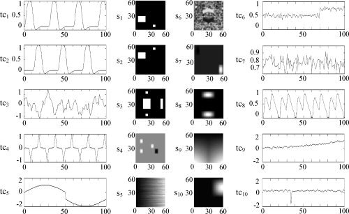
Ten fMRI‐like source images s 1–s 10 and the corresponding time courses tc1–tc10.
Preprocessing of fMRI‐Like Data and ICA Analysis
The fMRI‐like mixtures were reduced by principal component analysis (PCA) before performing ICA. Assuming that the number of sources is unknown without loss of generality, our criterion for determining the number is that at least 99.9% of the total variance of the mixed signals is retained after PCA reduction. This will ensure all the informative components are included. As a result, the fMRI‐like mixtures were reduced to 10 dimensions to retain 100% of the variance.
One standard blind ICA algorithm Infomax [Bell and Sejnowski,1995], which appears to have the best performance among several ICA algorithms including fastICA, JADE, and EVD for fMRI analysis [Correa et al.,2007], and the semiblind algorithm ICA‐R are included for comparison. For the Infomax algorithm, the learning rate was set to be 0.001. For the proposed algorithm and ICA‐R, we used G(y i) = exp(−y /2), ε(y i,r i) = −E{y i r i}, and ξi was initialized with a small value (e.g., ξi = 0.01) and then gradually increased to help the algorithm converge to the global maximum [Lu and Rajapakse,2005]. An actual scheme could be ξi = kξi, where k can be either the number of iteration or a constant (e.g., k = 100). We here applied the scheme ξi = 100ξi. However, through our simulations we found the algorithm was insensitive to the ξi update scheme. As ICA‐R is sensitive to the learning rate, we selected it through extensive simulations utilizing different values. The results showed that ICA‐R had consistent performance with a moderate learning rate (such as 0.01) but had less consistent performance with large values (such as 1 and 0.1) or with small ones (such as 0.001), we thus used a fixed learning rate 0.01.
Automatic Extraction of Sources of Interest
Assuming that s 1, s 2, and s 3 were three sources of interest. We generated three partially correct references r 1–r 3 for s 1–s 3 since prior information is usually not perfect. The accuracy of the reference can be defined as the normalized correlations of the references with the sources as the closeness measure ε(y i,r i) = −E{y i r i} is used. Figure 2 shows the three spatial references r 1–r 3 (the accuracy of r 1–r 3 is 93.8%, 93.8%, and 93.5%, respectively). Next, we used the proposed algorithm and ICA‐R to automatically extract s 1–s 3 by utilizing three references r 1–r 3 from the noiseless and noisy mixtures, respectively, but selected three corresponding signals from 10 estimates of Infomax using r 1–r 3.
Figure 2.
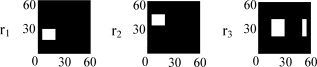
Three partially correct references r 1–r 3 for s 1–s 3.
To save space, we only show the results for a noisy case SNR = 0 dB in Figure 3. The proposed algorithm and ICA‐R automatically extracted three images (denoted as yi) and the time courses (denoted as t̂ci), as shown in Figure 3a,b. Figure 3c shows three selected images and the time courses estimated by Infomax. Compared with the three original sources s 1–s 3 and the time courses tc1–tc3 in Figure 1, we can see that all of the three ICA algorithms achieved good separation.
Figure 3.
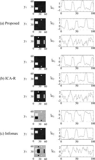
Images and time courses automatically extracted by the proposed algorithm (a) and ICA‐R (b) using the spatial references r 1–r 3, or selected from the estimates by Infomax (c) from noisy mixtures with SNR = 0 dB.
In addition, we generated an incorrect reference r4 (see Fig. 4a) to show what effect the use of prior information would have if the expected components did not actually exist in the data. For recognition, we used a noiseless mixture of s 1, s 2, s 3, s 4, s 6, s 7, s 8, and s 10, from which four components were extracted by using the four different spatial references r 1, r 2, r 3, and r 4. Figure 4b,c show the image y4 and time course t̂c4 extracted by the proposed algorithm and ICA‐R corresponding to the incorrect reference r4. We can see that the extracted images were actually mixtures of the original sources, and the extracted time courses were also noisy mixtures of the original time courses. This demonstrates that the proposed algorithm and ICA‐R do not generate artificial sources as a result of incorrect references. Note that the three images and time courses corresponding to r1‐r3 are much similar to those in Figure 3a,b but without noises (since the mixture is noiseless).
Figure 4.

An incorrect reference r 4 (a) and its corresponding image and time course extracted by the proposed algorithm (b) and ICA‐R (c) from noiseless mixtures by using four different spatial references r 1, r 2, r 3, and r 4.
To quantitatively compare the estimation quality of the three ICA algorithms, we computed the following signal‐to‐noise ratio (SNR) for the recovered sources:
| (15) |
where σ2 is the variance (power) of a source signal, mse denotes the mean square error between a source signal and its estimate (i.e., mse is the noise power). Figure 5 includes the results for the noiseless and noisy conditions. It can be found that the proposed algorithm has higher average SNR than ICA‐R and Infomax, while ICA‐R has higher average SNR than Infomax. This demonstrates that the proposed approach can further improve ICA performance by utilizing spatial prior information. We also examined how inaccurate the spatial reference could be, i.e., the effect of the reference accuracy on the estimation performance. Specifically, we compared the proposed approach with ICA‐R by using three spatial references r 1–r 3 with accuracy of 100%, 56%, and 38% under noiseless condition and three noise levels (SNR = 5, 0, −5 dB). Figure 6 shows the results, in which the SNR for Infomax in Figure 5 is also listed for comparison. We can see that the two semiblind algorithms achieve increased SNR with increased accuracy of references, and they have higher SNR than Infomax under noiseless and noisy conditions when the accuracy is above 56%. Compared with ICA‐R, the proposed algorithm significantly increased SNR when the accuracy of spatial reference was further increased and the noisy level for mixture was further decreased. Note that standard ICA outperforms the two semiblind algorithms when the spatial references are too rough, e.g., when the accuracy is 38%, Infomax is better than the proposed approach and ICA‐R in the noiseless case, but at the noise levels typical of fMRI performs at a similar level to the proposed approach (refer to Fig. 6c).
Figure 5.
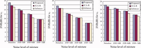
Comparison of SNR (dB), defined in Eq. (15), for estimates of s 1, s 2, and s 3 by the proposed approach, ICA‐R (using three partially correct references r 1–r 3), and Infomax under noiseless condition and three noise levels (SNR = 5, 0, −5 dB). [Color figure can be viewed in the online issue, which is available at www.interscience.wiley.com.]
Figure 6.

Comparison of SNR (dB), defined in Eq. (15), for estimates of s1, s2, and s3 by the proposed approach and ICA‐R by using three spatial references r 1–r 3 with accuracy of 100% (a), 56% (b), and 38% (c) under noiseless condition and three noise levels (SNR = 5, 0, −5 dB). The SNR (dB) for Infomax in Figure 5 is also listed for comparison. [Color figure can be viewed in the online issue, which is available at www.interscience.wiley.com.]
ANALYSIS OF REAL FMRI DATA AND RESULTS
Once the correctness of the proposed approach was confirmed by the simulation results, we applied it to real fMRI data from 11 subjects performing a visuo‐motor task to automatically extract components of interest.
Participants
Participants were recruited via advertisements, presentations at local universities, and by word‐of‐mouth. Eleven right‐handed participants with normal vision (five females, six males, average age 30 years) participated in the study. Participants provided written informed consent for a protocol approved by the Hartford Hospital Institutional Review Board.
Visuomotor Paradigms
A visuo‐motor task performed by the subjects involved two identical but spatially offset, periodic, visual stimuli, shifted by 20 s from one another. The visual stimuli were projected via an LCD projector onto a rear‐projection screen subtending approximately 25 degrees of visual field, visible via a mirror attached to the MRI head coil. The stimuli consisted of an 8Hz reversing checker board pattern presented for 15 s in the right visual hemifield, followed by 5 s of an asterisk fixation, followed by 15 s of checkerboard presented to the left visual hemifield, followed by 20 s of asterisk fixation. The 55 s set of events was repeated four times for a total of 220 s. The motor stimuli consisted of participants touching their thumb to each of their four fingers sequentially, back and forth, at a self‐paced rate using the hand on the same side on which the visual stimulus is presented.
Imaging Parameters
Scans were acquired at the Olin Neuropsychiatry Research Center at the Institute of Living on a Siemens Allegra 3T dedicated head scanner equipped with a 40mT/m gradients and a standard quadrature head coil. The functional scans were acquired using gradient‐echo planar imaging with the following parameters (repeat time, TR = 1.50 s; echo time, TE = 27 ms, field of view = 24 cm, acquisition matrix = 64 × 64, flip angle = 60 degrees, slice thickness = 4 mm, gap = 1 mm, 29 slices, ascending acquisition). Six “dummy” scans were performed at the beginning to allow for longitudinal equilibrium, after which the paradigm was automatically triggered to start by the scanner.
Preprocessing of fMRI Data
The fMRI data were preprocessed using SPM2. Images were realigned using INRIalign—a motion correction algorithm unbiased by the local signal changes [Freire and Mangin,2001; Freire et al.,2001]. Data were spatially normalized into the standard Montreal Neurological Institute (MNI) space [Friston et al.,1995], spatially smoothed with an 8 × 8 × 8 mm3 full width at half‐maximum Gaussian kernel. The data (originally acquired at 3.75 × 3.75 × 5 mm3) were slightly resampled to 3 × 3 × 5 mm3, resulting in 53 × 63 × 29 voxels.
The number of informative components (i.e., the total number of the sources M) included in each of 11 subjects of fMRI data was estimated according to the Akaike information criterion [Akaike,1974; Li et al.,2007], respectively. With the above‐mentioned criterion retaining 99.9% of the total variance, the estimated number M ranged from 14 to 20. We thus utilized the maximum number M = 20 as the final one. The fMRI data from each of the 11 subjects were then reduced by PCA to 20 dimensions.
Automatic Extraction of Components of Interest
Since the right and left task‐related components and the default mode component are signals of interest and their spatial information is available, we focus on extracting the three components (i.e., L = 3) out of 20 source signals with the three ICA algorithms, in which the same functions and parameters as above were used. We constructed the spatial references from the available atlases including Brodmann areas (BAs) and functional areas using WFU_PickAtlas [Lancaster et al.,1997, 2000; Maldjian et al.,2003], a tool that allows the user to create masks by selecting different areas of the brain. The labels were selected using the MNI atlases within the WFU_PickAtlas tool. Specifically, the two reference masks for the right and left task‐related components include BAs 1, 2, 3 (somatosensory area), BA 4 (primary motor area), BA 6 (secondary motor area), BA 17 (primary visual area), and BAs 18, 19 (secondary visual areas); the default mode reference is formed by BA 7 (posterior parietal cortex), BA 10 (anterior cingulate), BA 39 (occipitoparietal junction), Precuneus, and Posterior cingulated [Correa et al.,2007]. Figure 7 shows three created reference masks, which were smoothed with the same smoothing kernel used for the fMRI data.
Figure 7.
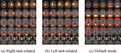
Three spatial reference masks corresponding to right task‐related component (a), left task‐related component (b), and default mode component (c).
With the three spatial references, the proposed algorithm and ICA‐R automatically extracted the two task‐related components and the default mode component from each of 11 subjects in the same order as that of the three references. In contrast, the three desired components needed to be selected out of 20 estimates by Infomax based on the three spatial references. Since the estimation consistency for multiple subjects can demonstrate the robustness of an ICA algorithm to individual subject differences, we performed a voxel‐wise one sample t‐test on each of the three estimated components over the 11 subjects (the individual subject components were first normalized to unit standard deviation), and then thresholded each of the t‐maps (voxel values are t‐values) at a false discovery rate (FDR) corrected q < 0.01 [Genovese et al.,2002]. Figure 8 shows the estimated t‐maps. We see that the proposed approach and Infomax obtain quite similar results for the right and left task‐related t‐maps but ICA‐R fails to reach significance. This is mainly caused by the sensitivity of Newton‐like learning to learning rate and initialization. Since we used a fixed learning rate and random initialization of the weight vectors, ICA‐R occasionally failed to extract the expected signals for several subjects. Table I presents the normalized spatial correlations of the three reference masks with the three estimated t‐maps for each of 11 subjects by the three ICA algorithms. We highlighted the very low correlations in bold black, which mean that the corresponding component was not found or was very noisy. We can see that ICA‐R did not find the right task‐related component from subject 5 and 9, and the left one from subject 1, 5, and 7. Note that the spatial correlation is a rough index to tell the correctness and the quality of the estimations, the same correlation values for different algorithms do not mean the estimated t‐maps are the same.
Figure 8.
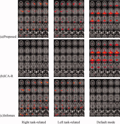
The estimated right and left task‐related t‐maps and default mode t‐maps by the proposed algorithm (a), ICA‐R (b), and Infomax (c) (thresholded at FDR corrected q < 0.01).
Table I.
Normalized spatial correlations of three reference masks with three estimated t‐maps for each of 11 subjects by three ICA algorithms
| Proposed | ICA‐R | Infomax | ||
|---|---|---|---|---|
| Right task‐related mask and 11 t‐maps | Subject 1 | 0.46 | 0.46 | 0.39 |
| Subject 2 | 0.54 | 0.54 | 0.48 | |
| Subject 3 | 0.53 | 0.52 | 0.47 | |
| Subject 4 | 0.43 | 0.43 | 0.36 | |
| Subject 5 | 0.53 | 0.23 | 0.46 | |
| Subject 6 | 0.54 | 0.50 | 0.50 | |
| Subject 7 | 0.49 | 0.49 | 0.43 | |
| Subject 8 | 0.56 | 0.56 | 0.46 | |
| Subject 9 | 0.44 | 0.27 | 0.37 | |
| Subject 10 | 0.56 | 0.56 | 0.44 | |
| Subject 11 | 0.43 | 0.43 | 0.26 | |
| Left task‐related mask and 11 t‐maps | Subject 1 | 0.45 | 0.29 | 0.36 |
| Subject 2 | 0.49 | 0.49 | 0.36 | |
| Subject 3 | 0.55 | 0.55 | 0.49 | |
| Subject 4 | 0.45 | 0.44 | 0.39 | |
| Subject 5 | 0.53 | 0.25 | 0.46 | |
| Subject 6 | 0.52 | 0.52 | 0.46 | |
| Subject 7 | 0.56 | 0.12 | 0.48 | |
| Subject 8 | 0.53 | 0.49 | 0.41 | |
| Subject 9 | 0.44 | 0.43 | 0.37 | |
| Subject 10 | 0.52 | 0.52 | 0.42 | |
| Subject 11 | 0.41 | 0.41 | 0.30 | |
| Default mode mask and 11 t‐maps | Subject 1 | 0.58 | 0.58 | 0.35 |
| Subject 2 | 0.54 | 0.54 | 0.23 | |
| Subject 3 | 0.58 | 0.58 | 0.30 | |
| Subject 4 | 0.57 | 0.57 | 0.37 | |
| Subject 5 | 0.63 | 0.63 | 0.51 | |
| Subject 6 | 0.56 | 0.56 | 0.30 | |
| Subject 7 | 0.56 | 0.56 | 0.41 | |
| Subject 8 | 0.57 | 0.57 | 0.31 | |
| Subject 9 | 0.45 | 0.45 | 0.25 | |
| Subject 10 | 0.57 | 0.56 | 0.26 | |
| Subject 11 | 0.61 | 0.61 | 0.41 |
The largest difference for constrained ICA and standard blind ICA occurs for the default mode network. The proposed algorithm and ICA‐R show activated regions consistent with the default mode reference in Figure 7c, whereas Infomax was significant for only several voxels of the default mode areas (other voxels become visible if a much lower threshold such as q < 0.1 was used, but the variability from subject to subject was much higher than the proposed algorithm and ICA‐R). From Table I we also see that Infomax failed to find the default mode component for three subjects and the other spatial correlations were also lower than the proposed approach and ICA‐R.
To further evaluate the three t‐maps, we computed the number of signal voxels (voxels which overlap with the corresponding masks, denoted as voxs), the number of noise voxels (voxels which do not overlap with the corresponding masks, denoted as voxn), and correspondingly defined a new SNR since we know nothing about the source signals needed by Eq. (15):
 |
(16) |
where t i(t j) denotes the t‐value of a signal voxel (noise voxel). Note that the number of activated voxels should be evaluated together with SNR because some noise voxels are included in the estimated maps. Table II and Table III record the results. We see that, among the three ICA algorithms, the proposed algorithm did not always produce the maximal number of activated voxels, but always gave the lowest number of noise voxels and the highest SNR, e.g., the percentage of the noise voxels included in the default mode t‐map is 1.72% for the proposed algorithm but is 9.31% for ICA‐R (refer to Table II).
Table II.
Comparison of the number of signal voxels (voxs) and the number of noise voxels (voxn) for three t‐maps estimated by three ICA algorithms
| Proposed | ICA‐R | Infomax | ||
|---|---|---|---|---|
| Right task‐related | voxs | 1739 | 0 | 1978 |
| voxn | 245 | 0 | 916 | |
| Left task‐related | voxs | 2178 | 0 | 1515 |
| voxn | 338 | 0 | 492 | |
| Default mode | voxs | 4397 | 7339 | 2 |
| voxn | 77 | 753 | 0 | |
Table III.
Comparison of SNR (dB), defined in Eq. (16), for three t‐maps estimated by three ICA algorithms
| Proposed (dB) | ICA‐R (dB) | Infomax (dB) | |
|---|---|---|---|
| Right task‐related | 16.07 | void | 10.97 |
| Left task‐related | 15.28 | void | 12.34 |
| Default mode | 24.10 | 16.44 | void |
To present a more fair comparison, we also compared the three ICA approaches when excluding the failed cases in Table I. Table IV shows the results. We see that the number of activated voxels becomes much lower than that in Table II while the SNR increases a little compared to that in Table III (this is reasonable since the percentage of the noise voxels in Table IV decreases a little compared with that in Table II), the two constrained ICA algorithms have better SNR than Infomax, and the proposed approach always provides a higher SNR than ICA‐R and a comparable number of activated voxels to the largest number of voxels. These results further confirm the advantages of the proposed approach over ICA‐R separately from the Newton‐like learning problem.
Table IV.
Comparison of the number of signal voxels (voxs), the number of noise voxels (voxn), and SNR (dB) defined in Eq. (16) for three t‐maps estimated by three ICA algorithms excluding the failed cases of ICA‐R in Table I
| Proposed | ICA‐R | Infomax | |||||||
|---|---|---|---|---|---|---|---|---|---|
| voxs | voxn | SNR (dB) | voxs | voxn | SNR (dB) | voxs | voxn | SNR (dB) | |
| Right task‐related | 620 | 61 | 17.27 | 516 | 66 | 15.73 | 884 | 381 | 11.15 |
| Left task‐related | 695 | 57 | 17.75 | 342 | 57 | 14.82 | 273 | 60 | 13.93 |
To evaluate the quality of the estimated time courses, we obtained the average time courses over the 11 subjects after normalizing the individual time courses to zero mean and unit variance. Figure 9a,b show the right and left task‐related average time courses estimated by the proposed algorithm (solid), ICA‐R (dash‐dot), and Infomax (dotted). We see that the three ICA algorithms obtain quite similar results to the two model time courses tc1 and tc2 (see Fig. 1). The difference is that the proposed algorithm has the lowest amplitudes during the alternate stimuli (e.g. left for the right task‐related component, or vice versa), and hence has the least crosstalk between the right and left tasks, and thus the lowest number of noise voxels in the t‐maps (see Table II). In addition, we compared the standard deviations of the individual default mode time course estimated by the three ICA algorithms over the 11 subjects. Figure 10 shows the average time courses (thick lines) and the error bound (dotted lines). It can be seen that the proposed algorithm and ICA‐R have lower deviation (dotted lines) than Infomax. As a result, the two semiblind ICA algorithms produced more significant t‐maps than Infomax (see Fig. 8).
Figure 9.
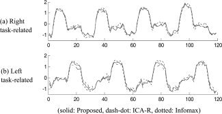
The right (a) and left (b) task‐related average time courses estimated by the proposed algorithm (solid), ICA‐R (dash‐dot), and Infomax (dotted).
Figure 10.

The average time courses (thick lines) and the error bound (dotted lines) for default mode component estimated by the proposed algorithm (a), ICA‐R (b), and Infomax (c). [Color figure can be viewed in the online issue, which is available at www.interscience.wiley.com.]
Finally, we compared the average one‐component estimation time for the three ICA algorithms to quantitatively compare the computational complexity of the proposed algorithm with the other two algorithms. The results are 0.68 s, 2.79 s, and 11.13 s, respectively. That is, the speed of our method is at least four times faster than ICA‐R and 16 times faster than Infomax. Therefore, the proposed algorithm considerably reduces the computational load due to fixed‐point learning. This is especially valuable for time sensitive applications, like real‐time ICA of fMRI data, or when analyzing large data sets, such as in group analyses.
DISCUSSION AND CONCLUSIONS
We have developed an efficient semiblind spatial ICA algorithm utilizing spatial information within the framework of constrained ICA with fixed‐point learning. Results for synthetic data and real fMRI data show that the proposed algorithm has improved SNR, robustness, and speed compared to the ICA‐R algorithm with Newton‐like learning and to the standard blind ICA algorithm Infomax by virtue of using spatial prior information.
The default mode component is of increasing interest in fMRI studies. We know that the group ICA algorithm [Calhoun et al.,2001] provides a way to reliably estimate the default mode maps by utilizing a large amount of information from a group of subjects [Correa et al.,2007]. However, if one is interested in performing ICA separately for each subject, reliable detection of the default mode network decreases. It is likely that noise and the fact that less data are being used to estimate the components are causing the problem. The proposed algorithm and ICA‐R were found to detect a significantly improved default mode component from a small amount of data from a single subject due to the use of spatial prior information.
The use of temporal priors for a semiblind ICA is justified when consistently or transiently task‐related components are of major interest compared with nontask related components. The use of spatial information can be justified in the same way since we are interested in identifying a well‐described network, but do not know its exact form (analogous to the case of transiently task‐related time courses). In this case, this well‐described network can be used as a spatial constraint; our approach can then be directly used to improve results. The spatial reference can be generated in other ways as well. For example, it can be derived from a network consistently identified from some other data (such as a component produced by ICA). In our experience, even the transiently task‐related components show fairly consistent spatial patterns, hence making this information available for a spatial reference. The use of spatial priors is also possible for resting‐state fMRI studies (for which we do not have temporal priors) due to the presence of commonly occurring spatial networks such as the default mode network. Because of consistency of the spatial patterns across subjects, data sets, and different fMRI tasks [Calhoun et al.,2008a, b; Franco et al.,2009], it is straightforward to generate spatial references which have high accuracy for spatial semiblind spatial ICA to improve performance.
In summary, we have presented the first application of spatial constraints within spatial ICA to fMRI data. Results indicate a significant improvement can be obtained over standard blind ICA approaches. In addition we have presented an improved semiblind ICA algorithm which is robust to initial conditions and computationally efficient. Given the increasing interest in identifying temporally coherent networks with consistent spatial patterns (such as default mode), the approach we present has wide applicability to study healthy as well as diseased brain.
Derivation of Eq. (11) from Eqs. (8) and (9)
For clarity, the Eq. (8) can be rewritten as:
| (A1) |
where  . The gradient of L(W,μ) is given by [Lu and Rajapakse, 2005]:
| (A2) |
where  , and
, and  . Let ρi = ρ(E{G(y
i)} − E{G(ν)}), we have J′(y) = 2ρi
G′ (w
i
x).
. Let ρi = ρ(E{G(y
i)} − E{G(ν)}), we have J′(y) = 2ρi
G′ (w
i
x). 
 , and
, and
we have C′ (y : W, μ) = μi g′ (y i : w i) in which μi = max {μi + γi g i(y i : w i),0}. Hence, (A2) becomes
| (A3) |
From the Eq. (9), the gradient of F(‖W‖2) can be expressed as:
| (A4) |
where  . Substituting (A3) and (A4) into the Eq. (10), we can obtain the Eq. (11).
REFERENCES
- Akaike H ( 1974): A new look at statistical model identification. IEEE Trans Automat Contr 19: 716–723. [Google Scholar]
- Beckmann CF, DeLuca M, Devlin JT, Smith SM ( 2005): Investigations into resting‐state connectivity using independent component analysis. Philos Trans R Soc Lond B Biol Sci 360: 1001–1013. [DOI] [PMC free article] [PubMed] [Google Scholar]
- Bell AJ, Sejnowski TJ ( 1995): An information‐maximization approach to blind separation and blind deconvolution. Neural Comput 7: 1129–1159. [DOI] [PubMed] [Google Scholar]
- Biswal BB, Ulmer JL ( 1999): Blind source separation of multiple signal sources of FMRI data sets using independent component analysis. J Comput Assist Tomogr 23: 265–271. [DOI] [PubMed] [Google Scholar]
- Calhoun VD, Adali T ( 2006): Unmixing fMRI with independent component analysis. IEEE Eng Med Biol Mag 25: 79–90. [DOI] [PubMed] [Google Scholar]
- Calhoun VD, Adali T, Pearlson GD, Pekar JJ ( 2001): A method for making group inferences from functional MRI data using independent component analysis. Hum Brain Mapp 14: 140–151. [DOI] [PMC free article] [PubMed] [Google Scholar]
- Calhoun VD, Adali T, Stevens MC, Kiehl KA, Pekar JJ ( 2005): Semi‐blind ICA of fMRI: A method for utilizing hypothesis‐derived time courses in a spatial ICA analysis. Neuroimage 25: 527–538. [DOI] [PubMed] [Google Scholar]
- Calhoun VD, Kiehl KA, Pearlson GD ( 2008a) Modulation of temporally coherent brain networks estimated using ICA at rest and during cognitive tasks. Hum Brain Mapp 29: 828–838. [DOI] [PMC free article] [PubMed] [Google Scholar]
- Calhoun VD, Pearlson GD, Maciejewski P, Kiehl KA ( 2008b) Temporal lobe and ‘default’ hemodynamic brain modes discriminate between schizophrenia and bipolar disorder. Hum Brain Mapp 29: 1265–1275. [DOI] [PMC free article] [PubMed] [Google Scholar]
- Cardoso JF ( 1998): Blind signal separation: Statistical principles. Proc IEEE 86: 2009–2025. [Google Scholar]
- Cichocki A, Amari S ( 2003): Adaptive Blind Signal and Image Processing: Learning Algorithms and Applications. New York: John Wiley. [Google Scholar]
- Cordes D, Haughton VM, Arfanakis K, Wendt GJ, Turski PA, Moritz CH, Quigley MA, Meyerand ME ( 2000): Mapping functionally related regions of brain with functional connectivity MR imaging. Am J Neuroradiol 21: 1636–1644. [PMC free article] [PubMed] [Google Scholar]
- Correa N, Adali T, Calhoun VD ( 2007): Performance of blind source separation algorithms for FMRI analysis. Magn Reson Imaging 25: 684–694. [DOI] [PMC free article] [PubMed] [Google Scholar]
- Damoiseaux JS, Rombouts SARB, Barkhof F, Scheltens P, Stam CJ, Smith SM, Beckmann CF ( 2006): Consistent resting‐state networks across healthy subjects. Proc Natl Acad USA 103: 13848–13853. [DOI] [PMC free article] [PubMed] [Google Scholar]
- De Martino F, Gentile F, Esposito F, Balsi M, Di Salle F, Goebel R, Formisano E ( 2007): Classification of fMRI independent components using IC‐fingerprints and support vector machine classifiers. Neuroimage 34: 177–194. [DOI] [PubMed] [Google Scholar]
- Franco AR, Pritchard A, Calhoun VD, Mayer AR ( 2009): Inter‐rater and inter‐method reliability of default mode network selection. Hum Brain Mapp 30: 2293–2303. [DOI] [PMC free article] [PubMed] [Google Scholar]
- Freire L, Mangin JF ( 2001): Motion correction algorithms may create spurious activation in the absence of subject motion. Neuroimage 14: 709–722. [DOI] [PubMed] [Google Scholar]
- Freire L, Roche A, Mangin JF ( 2001): What is the best similarity measure for motion correction in fMRI time series? IEEE Trans Med Imaging 21: 470–484. [DOI] [PubMed] [Google Scholar]
- Friston K, Ashburner J, Frith CD, Poline JP, Heather JD, Frackowiak RS ( 1995): Spatial registration and normalization of images. Hum Brain Mapp 2: 165–189. [Google Scholar]
- Garrity A, Pearlson GD, McKiernan K, Lloyd D, Kiehl KA, Calhoun VD ( 2007): Aberrant ‘default mode’ functional connectivity in schizophrenia. Am J Psychiatry 164: 450–457. [DOI] [PubMed] [Google Scholar]
- Genovese CR, Lazar NA, Nichols T ( 2002): Thresholding of statistical maps in functional neuroimaging using the false discovery rate. Neuroimage 15: 870–878. [DOI] [PubMed] [Google Scholar]
- Greicius MD, Krasnow B, Reiss AL, Menon V ( 2003): Functional connectivity in the resting brain: A network analysis of the default mode hypothesis. Proc Natl Acad Sci USA 100: 253–258. [DOI] [PMC free article] [PubMed] [Google Scholar]
- Greicius MD, Srivastava G, Reiss AL, Menon V ( 2004): Default‐mode network activity distinguishes Alzheimer's disease from healthy aging: Evidence from functional MRI. Proc Natl Acad Sci USA 101: 4637–4642. [DOI] [PMC free article] [PubMed] [Google Scholar]
- Hesse CW, James CJ ( 2006): On semi‐blind source separation using spatial constraints with applications in EEG analysis. IEEE Trans Biomed Eng 53: 2525–2534. [DOI] [PubMed] [Google Scholar]
- Hyvärinen A ( 1997): A family of fixed‐point algorithms for independent component analysis In: Proc IEEE Int. Conf. on Acoustics, Speech and Signal Processing (ICASSP'97). Munich, Germany: pp 3917–3920. [Google Scholar]
- Hyvärinen A ( 1998): New approximations of differential entropy for independent component analysis and projection pursuit In: Jordan MI, Kearns MJ, Solla SA, editors. Advances in Neural Information Processing Systems 10. MA: MIT Press; pp 273–279. [Google Scholar]
- Hyvärinen A, Karhunen J, Oja E ( 2001): Independent Component Analysis. New York: John Wiley. [Google Scholar]
- Lancaster JL, Summerln LJ, Rainey L, Freitas CS, Fox PT ( 1997): The Talairach Daemon, a database server for Talairach atlas labels. Neuroimage 5: S633. [Google Scholar]
- Lancaster JL, Woldorff MG, Parsons LM, Liotti M, Freitas CS, Rainey L, Kochunov PV, Nickerson D, Mikiten SA, Fox PT ( 2000): Automated Talairach atlas lables for functional brain mapping. Hum Brain Mapp 10: 120–131. [DOI] [PMC free article] [PubMed] [Google Scholar]
- Li Y, Adali T, Calhoun VD ( 2007): Estimating the number of independent components for fMRI Data. Hum Brain Mapp 28: 1251–1266. [DOI] [PMC free article] [PubMed] [Google Scholar]
- Lu W, Rajapakse JC ( 2000): Constrained independent component analysis In: Leen TK, Dietterich TG, Tresp V, editors. Advances in Neural Information Processing Systems 13 (NIPS2000). MA: MIT Press; pp 570–576. [Google Scholar]
- Lu W, Rajapakse JC ( 2003): Eliminating indeterminacy in ICA. Neurocomputing 50: 271–290. [Google Scholar]
- Lu W, Rajapakse JC ( 2005): Approach and applications of constrained ICA. IEEE Trans Neural Netw 16: 203–212. [DOI] [PubMed] [Google Scholar]
- Luenberger DG ( 1969): Optimization by Vector Space Methods. New York: John Wiley & Sons, Inc. [Google Scholar]
- Maldjian JA, Laurienti PJ, Kraft RA, Burdette JH ( 2003): An automated method for neuroanatomic and cytoarchitectonic atlas‐based interrogation of fMRI data sets. Neuroimage 19: 1233–1239. [DOI] [PubMed] [Google Scholar]
- McKeown MJ, Makeig S, Brown GG, Jung TP, Kindermann SS, Bell AJ, Sejnowski TJ ( 1998): Analysis of fMRI data by blind separation into independent spatial components. Hum Brain Mapp 6: 160–188. [DOI] [PMC free article] [PubMed] [Google Scholar]
- McKiernan KA, Kaufman JN, Kucera‐Thompson J, Binder JR ( 2003): A parametric manipulation of factors affecting task‐induced deactivation in functional neuroimaging. J Cogn Neurosci 15: 394–408. [DOI] [PubMed] [Google Scholar]
- Raichle ME, MacLeod AM, Snyder AZ, Powers WJ, Gusnard DA, Shulman GL ( 2001): A default mode of brain function. Proc Natl Acad Sci USA 98: 676–682. [DOI] [PMC free article] [PubMed] [Google Scholar]