

Abstract
Purpose
To investigate whether combining optic disc topography and short-wavelength automated perimetry (SWAP) data improves the diagnostic accuracy of relevance vector machine (RVM) classifiers for detecting glaucomatous eyes compared to using each test alone.
Methods
One eye of 144 glaucoma patients and 68 healthy controls from the Diagnostic Innovations in Glaucoma Study were included. RVM were trained and tested with cross-validation on optimized (backward elimination) SWAP features (thresholds plus age; pattern deviation (PD); total deviation (TD)) and on Heidelberg Retina Tomograph II (HRT) optic disc topography features, independently and in combination. RVM performance was also compared to two HRT linear discriminant functions (LDF) and to SWAP mean deviation (MD) and pattern standard deviation (PSD). Classifier performance was measured by the area under the receiver operating characteristic curves (AUROCs) generated for each feature set and by the sensitivities at set specificities of 75%, 90% and 96%.
Results
RVM trained on combined HRT and SWAP thresholds plus age had significantly higher AUROC (0.93) than RVM trained on HRT (0.88) and SWAP (0.76) alone. AUROCs for the SWAP global indices (MD: 0.68; PSD: 0.72) offered no advantage over SWAP thresholds plus age, while the LDF AUROCs were significantly lower than RVM trained on the combined SWAP and HRT feature set and on HRT alone feature set.
Conclusions
Training RVM on combined optimized HRT and SWAP data improved diagnostic accuracy compared to training on SWAP and HRT parameters alone. Future research may identify other combinations of tests and classifiers that can also improve diagnostic accuracy.
Keywords: machine learning classifier, neural networks, glaucoma, visual function, optic disc, structure-function relationship
Diagnosis and staging of glaucoma rely on both structural evaluation of the optic nerve and functional assessment of the visual field1. Several studies have documented the ability of confocal scanning laser ophthalmoscopy optic disc topographic measurements to discriminate between healthy and glaucomatous eyes2-4. Function-specific tests of visual function have been shown to be more sensitive to glaucomatous damage than standard automated perimetry (SAP)5-7. Short-wavelength automated perimetry (SWAP), for example, targets the blue-yellow pathway and may detect glaucomatous damage up to five years earlier than SAP8. A recent study has shown that the sensitivity to detect glaucoma can be improved by combining data from structural and function-specific tests9.
In efforts to summarize the large amount of data produced by structural and functional tests, various types of pattern-recognition algorithms known as machine learning classifiers have been applied to optic disc imaging results and visual field data. Machine learning classifiers (MLCs) are well suited for evaluating these large data sets, because they are able to detect complex patterns and trends. Several types of MLCs have been applied to glaucoma, including the mixture of Gaussian (MoG), sub-space mixture of Gaussian (SS-MoG), support vector machine (SVM) and the relevance vector machine (RVM). The RVM classifier incorporates a probabilistic output and has previously been shown to perform as well as the support vector machine (SVM) classifier10. This probabilistic output allows for an intuitive interpretation of the RVM results and may provide a particularly useful clinical perspective. Using either structural10, 11 or functional12-15 measurements alone, machine learning classifiers showed similar or better diagnostic accuracy for glaucoma than traditional analyses. A few studies have reported an improvement in the ability of machine learning classifiers to detect glaucoma when they are trained using standard automated perimetry (SAP) and structural measurements16-19, compared to when they are trained with either data in isolation.
Bowd et al19 reported that combining optical coherence tomography (OCT) and SAP data resulted only in a marginal improvement in the ability of machine learning classifiers to classify eyes as glaucomatous or healthy. This study may have been somewhat biased by the use of SAP to both classify the eyes and train the machine learning classifiers. This problem is a consequence of the inexistence of a gold standard for glaucoma and is very difficult to overcome when studying structure and function simultaneously. In the present study, we reduced the classification bias by using different measures to classify the eyes and train the machine learning classifier. Our purpose was to determine whether combining structural and functional data improves the diagnostic accuracy of relevance vector machine (RVM) classifiers for detecting glaucomatous eyes compared to using each test alone.
METHODS
Participants
One randomly selected eye of each of 212 participants (144 glaucoma patients and 68 healthy controls) over the age of 40 years was included in this study. All participants were enrolled in the Diagnostic Innovations in Glaucoma Study (DIGS), an ongoing prospective longitudinal study of patients with primary open-angle glaucoma. Participants were evaluated at the Hamilton Glaucoma Center, University of California, San Diego. Informed consent was obtained from all participants and the Human Research Protections Program at the University of California at San Diego approved all methodology. This observational cross-sectional study adhered to the declaration of Helsinki for research involving human subjects and was performed in conformity with the Health Insurance Portability and Accountability Act (HIPAA).
All participants underwent complete ophthalmologic examinations including slitlamp biomicroscopy, intraocular pressure (IOP) measurement, and dilated stereoscopic fundus examination. Simultaneous stereoscopic photographs with good clarity and stereopsis were obtained for all participants. At study entry, all participants had open angles, a best corrected acuity of 20/40 or better, a spherical refraction within ±5.0 D, and cylinder correction within ±3.0 D. Family history of glaucoma was allowed. Participants were excluded if they had a history of intraocular surgery except for uncomplicated cataract or glaucoma surgery. We also excluded all participants with non-glaucomatous secondary causes of elevated IOP (e.g. iridocyclitis, trauma), other intraocular eye disease, and other diseases with a potential impact on the visual field (e.g. pituitary lesions, demyelinating diseases, HIV+ or AIDS, or diabetic retinopathy). Participants taking medications known to affect visual field sensitivity or with problems other than glaucoma affecting color vision were also excluded.
All participants underwent SAP, SWAP, HRT II optic disc imaging and IOP measurements within a six-month window. Simultaneous stereophotographs were usually available within 6 months of SWAP. When sterophotographs were unavailable within that time frame, we included participants with stereophotographs taken at any time interval if there was evidence of glaucoma on photos taken prior to SWAP (for glaucoma patients) or no evidence of glaucoma on photos taken after SWAP (for healthy controls). All SWAP and SAP visual fields were reliable (less than 33% fixation losses, false negative errors, and false positive errors). Abnormal SAP visual fields were confirmed by abnormal results on a prior or subsequent SAP test. All HRT images were reviewed by trained examiners and were of good quality, requiring focused reflectance with a standard deviation no greater than 50 μm. The mean ± SD for the standard deviation of the topography was 20.38 ± 8.99 in the group of glaucoma patients, and 16.16 ± 4.99 in the healthy control group. Participants with normal visual fields and healthy appearing optic discs on stereophotographs who had abnormal funduscopic examinations or elevated intraocular pressures (IOP ≥ 23mm Hg) were excluded from this study.
Healthy eyes were defined as those with a healthy appearance of the optic disc on simultaneous stereophotographs and clinical fundus examination, normal results on SAP visual fields, and IOP ≤ 22 mm Hg. Glaucomatous eyes were defined as those with glaucomatous optic neuropathy on stereophotographs and/or two consecutive abnormal SAP visual fields. Twenty-three eyes were identified as glaucomatous by visual fields alone, 78 by stereophotographs alone, and 43 by both visual fields and stereophotographs. Glaucomatous eyes were defined based on either visual field or glaucomatous optic neuropathy to avoid biasing the results towards either the structural or functional tests. The results obtained in two separate clinical trials show that in some patients, visual field defects are detected prior to the appearance of glaucomatous optic neuropathy. In the Ocular Hypertension Treatment Study (OHTS), 35% of the patients who reached the study endpoint showed visual field defect and no optic disc abnormality.20 A similar finding was observed in the European Glaucoma Prevention Study (EGPS), where 60% of the patients who reached the study endpoint showed visual field loss only.21
Visual function measures
SAP visual field testing
SAP results were used only to satisfy the inclusion criteria and not to train RVM. SAP was performed on the Humphrey Visual Field Analyzer (Carl Zeiss Meditec, Dublin, CA). A Goldmann size III (0.43°) stimulus was projected on a 31.5-apostilb background. Fifty-four locations were tested with the 24−2 program. The two locations within the blind spot were excluded from the analysis, leaving 52 test locations. To satisfy the inclusion criteria, participants were tested with either the full-threshold (FT) algorithm or the Swedish Interactive Thresholding Algorithm (SITA). Individual thresholds were compared to the manufacturer's internal normative database. SAP visual fields were considered abnormal if the pattern standard deviation (PSD) probability was < 5% or if the glaucoma hemifield test (GHT) was outside normal limits.
SWAP visual field testing
SWAP measurements were used to train RVM classifiers. They were not used as inclusion criteria. SWAP (Humphrey Field Analyzer, Carl Zeiss Meditec, Dublin, CA) was performed using procedures previously reported to be optimal22. Briefly, a Goldmann size V blue stimulus was presented on a 100 cd/m2 yellow background. As with SAP, the two locations within the blind spot were discarded. The full-threshold algorithm and 24−2 stimulus presentation pattern were used for all participants. Individual thresholds were compared with the SWAP normative database developed in our laboratory (N=345).23
Structural measures
Stereoscopic photographs
Color simultaneous stereoscopic photographs were obtained using a Topcon camera (TRC-SS, Topcon Instrument Corp of America, Paramus, NJ) after maximal pupillary dilation. Photographs were independently assessed by two trained graders, masked to the diagnosis of the participant and to the evaluation of the other grader. In cases where the two graders disagreed, a third experienced grader served as an adjudicator. Stereophotographs were evaluated using a stereoscopic viewer (Pentax Stereo Viewer II, Asahi Optical Co.-Pentax, Tokyo, Japan) illuminated with color-corrected fluorescent lighting. Glaucomatous optic neuropathy was defined by evidence of any of the following: excavation, neuroretinal rim thinning or notching, nerve fiber layer defects, or an asymmetry of the vertical cup/disc ratio ≥ 0.2 between the two eyes.
Optic disc topography
Optic disc topography parameters were obtained with the Heidelberg Retina Tomograph (HRT) II, version 2.01 (Heidelberg Engineering, Dossenheim, Germany) confocal scanning laser ophthalmoscope (CSLO) as previously described24. A 670-nm wavelength diode laser sequentially scanned the retinal surface in consecutive focal planes to construct reproducible three-dimensional topographic image25, 26. Three 15° scans centered on the optic disc judged to be of acceptable quality were obtained for each test eye. These scans were used to create a mean topography image for analysis. An experienced examiner outlined the optic disc margin on the mean topographic image while viewing stereoscopic photographs of the optic disc. Each image was assessed for quality by trained examiners. From these images, the HRT II software derived a set of global and regional topographic parameters as well as the Moorfield regression analysis, which have shown a good ability to discriminate between healthy controls and patients with early glaucoma27-29.
Machine Learning Classifier
This study used a supervised relevance vector machine (RVM) classifier implemented with the SparseBayes algorithm (version 1.0) (Microsoft Research, Cambridge, UK, for MatLab, The MathWorks). RVM is a classification method that uses a Bayesian model to minimize classification errors without requiring a statistical model. By mapping data into a higher dimensional space, RVM can use a hyperplanar boundary to separate data that might be poorly separated by a hyperplanar boundary in the original lower-dimensional space. RVM finds a hyperplane that maximizes the distance between a sparse selection of examples of healthy and glaucomatous eyes that are difficult to classify. The internal parameters successively self-adjust against a pre-defined gold standard until the classification performance no longer improves. The RVM classifier has previously been shown to perform as well as the support vector machine (SVM) classifier in the diagnosis of glaucoma based on scanning laser polarimetry input10. The RVM uses a sparser decision function than SVM, which requires more decision points to minimize training error and maximize smoothness. Because RVM depends on fewer input examples to generate the decision surface, it may classify better than SVM when only a small sample set is available for training. The RVM also has the advantage of generating a probability of glaucoma. This probability of class membership is more intuitive than the non-probabilistic output of SVM.
Analyses
Receiver operating characteristic (ROC) curves for classifying eyes as glaucomatous or healthy were generated for RVM trained and tested on HRT parameters alone, SWAP parameters alone and combined HRT and SWAP parameters. The HRT parameters included the eighty global (360°) and regional topographic parameters listed in Table 1. Regions were defined as temporal superior (46−90° unit circle), nasal superior (91−135°), nasal (136−225°), nasal inferior (226−270°), temporal inferior (271−315°), and temporal (316−45°). Three different sets of SWAP parameters were used: 1) thresholds in decibels plus age, 2) pattern deviation (PD) values in decibels, and 3) total deviation (TD) values in decibels at 52 test locations. While SWAP thresholds and TD values are sensitive to the presence of cataracts, cloudy media and small pupils, SWAP PD values incorporate adjustments for these factors. When the RVM classifier was trained on SWAP parameters alone, each SWAP data set was evaluated independently. When the RVM classifier was trained on combined data, each SWAP data set was combined to the HRT data and evaluated in separate sessions. Finally, the RVM classifier was also trained and tested on the two linear discriminant function (LDF) formulas available on the HRT and developed by R. Burke et al (RB) and F.S. Mikelberg et al30 (FSM) and on two SWAP global indices (mean deviation, MD; pattern standard deviation, PSD). Statistically significant differences between the AUROCs were determined using the method of DeLong et al31. Sensitivities at 75%, 90% and 96% specificities were calculated. These specificity levels were selected arbitrarily to represent moderate to high specificity levels.
Table 1.
Twelve global and 68 regional HRT parameters included in the full-dimensional HRT input set.
| Parameter | Location |
|---|---|
| Optic disc area (mm2) | (Global, T, TS, TI, N, NS, NI) |
| Area below reference (cup area) (mm2) | (Global, T, TS, TI, N, NS, NI) |
| Mean height contour (mm) | (Global, T, TS, TI, N, NS, NI) |
| Height variation contour (mm) | (Global, T, TS, TI, N, NS, NI) |
| Contour line modulation (mm) | (TI, TS) |
| Volume below reference (mm3) | (Global, T, TS, TI, N, NS, NI) |
| Volume above reference (mm3) | (Global, T, TS, TI, N, NS, NI) |
| Cup shape | (Global, T, TS, TI, N, NS, NI) |
| Mean cup depth (mm) | (Global, T, TS, TI, N, NS, NI) |
| Mean RNFL thickness (mm2) | (Global, T, TS, TI, N, NS, NI) |
| Reference height (mm) | (Global) |
| Rim area (mm) | (Global, T, TS, TI, N, NS, NI) |
| Rim-to-disc area ratio | (Global, T, TS, TI, N, NS, NI) |
T: temporal; TS: temporo-superior; TI: temporo-inferior; N: nasal; NS: naso-superior; NI: naso-inferior
Ideally, the RVM would be trained using a data set independent from that on which it is tested. This, however, requires a large sample that was not available in the present study. Instead, for each ROC curve, a ten-fold cross-validation technique was used to train and test the RVM classifiers to reduce the bias of estimation of ROC areas. The glaucoma and healthy groups were divided into ten approximately equal and mutually exclusive subsets. The RVM classifier was trained on nine of the subsets and tested on the tenth subset. This routine was repeated ten times such that each subset served as the test set once. The test set was never included in its own training set. The results from the ten test sets were combined to generate a single receiver ROC curve.
Feature Selection using Backward Elimination
Our data set was composed of a large number of parameters, with relatively few observations (N=212) per parameter. The performance of machine learning classifiers can be reduced by the inclusion of irrelevant parameters32. In addition to training and testing the RVM classifier on the full dimensional (FD) feature set including all parameters listed in Table1, we achieved dimension reduction by applying the backward elimination feature selection technique to identify a near-optimal subset of features. Previous work has shown that backward elimination tended to produce more effective near-optimal subsets than forward selection2. Beginning with a full feature set, we deleted the features that least affected the performance of the RVM classifier. This process was repeated until the feature set was empty. The AUROC curves were plotted with the x-axis showing the number of features included. For each data set, we included the number of features that yielded the highest AUROC (i.e. “peaking”). It is important to emphasize that due to the order in which each parameter is selected for elimination, backward elimination optimization yields a group of features that are not necessarily in decreasing order of value to classification. Some features, which may be equally valuable compared to those at the top of the list, are eliminated because they provide similar information to the features that remain on the list.
To minimize feature selection bias, internal and external cross-validation techniques were used as previously described2. In brief, the full data set was divided into five partitions, with four partitions comprising the feature selection set and the remaining partition serving as an independent evaluation set for external cross-validation. Backward elimination was applied to the feature selection set, using ten-fold internal cross-validation as described above. The resultant AUROC curve was used to rank the parameters. The entire process was repeated five times, yielding five different parameter rankings. A weighted average of the rankings was calculated to produce a ranked list of features. The number of features at which the AUROC curve reached its “peak” was determined and these features were used in our optimized input data set.
RESULTS
Table 2 compares the mean values for demographic characteristics, SWAP MD and PSD, and each global HRT parameter between the glaucoma and healthy study groups (JMP software, SAS Institute, Cary, NC). The variables were analyzed using the Chi-square test (for categorical variables), Mann-Whitney U test (for continuous variables that did not meet the assumptions of normality and equal variance), and t-test (for continuous variable that met the assumptions of normality and equal variance). The assumptions of normality and equal variance were tested using the Shapiro-Wilk and Brown-Forsythe tests, respectively. Statistically significant differences were found for all parameters except height variation contour (p=0.15). The healthy controls were on average four years younger than the glaucoma patients (p=0.01).
Table 2.
Descriptive characteristics of the glaucoma and healthy study groups are presented.
| Glaucomatous Eyes (N=144) | Healthy Eyes (N=68) | p-value | |
|---|---|---|---|
| Age (yrs, mean ± SD, range) | 62.0 ± 10.1 (39.6−85.3) | 58.0 ± 9.9 (40.0−86.9) | 0.01* |
| Gender (% male) | 45% | 35% | 0.17† |
| SWAP MD (Mean ± SD) (dB) | −5.19 ± 4.62 | −2.59 ± 3.40 | <0.0001‡ |
| SWAP MD Range (dB) | −25.55 to 3.83 | −17.26 to 3.85 | |
| SWAP PSD (Mean ± SD) (dB) | 4.39 ± 2.07 | 2.99 ± 0.73 | <0.0001‡ |
| SWAP PSD Range (dB) | 1.90 to 11.95 | 1.49 to 4.71 | |
| Optic disc area (mm2) | 2.12 ± 0.46 (1.12−3.31) | 1.77 ± 0.36 (1.14−2.85) | <0.0001‡ |
| Area below reference (cup area) (mm2) | 0.86 ± 0.44 (0.00−2.09) | 0.32 ± 0.26 (0.00−0.96) | <0.0001‡ |
| Mean height contour (mm) | 0.18 ± 0.10 (−0.18−0.53) | 0.06 ± 0.09 (−0.15−0.32) | <0.0001* |
| Height variation contour (mm) | 0.39 ± 0.10 (0.13−0.80) | 0.41 ± 0.12 (0.18−0.86) | 0.15* |
| Volume below reference (mm3) | 0.23 ± 0.19 (0.00−0.91) | 0.07 ± 0.08 (0.00−0.31) | <0.0001‡ |
| Volume above reference (mm3) | 0.31 ± 0.15 (0.04−0.93) | 0.42 ± 0.17 (0.15−1.14) | <0.0001* |
| Cup shape | −0.12 ± 0.08 (−0.30−0.13) | −0.20 ± 0.06 (−0.35--0.08) | <0.0001* |
| Mean cup depth (mm) | 0.28 ± 0.11 (0.01−0.71) | 0.18 ± 0.09 (0.04−0.41) | <0.0001* |
| Mean RNFL thickness (mm2) | 0.21 ± 0.09 (−0.03−0.50) | 0.27 ± 0.08 (0.13−0.58) | <0.0001* |
| Reference height (mm) | 0.40 ± 0.12 (0.03−0.80) | 0.34 ± 0.13 (0.09−0.74) | 0.002* |
| Rim area (mm) | 1.26 ± 0.34 (0.40−2.40) | 1.45 ± 0.32 (0.83−2.41) | 0.0002* |
| Rim-to-disc area ratio | 0.61± 0.16 (0.20−1.00) | 0.82 ± 0.13 (0.48−1.00) | <0.0001* |
All HRT parameters refer to global measurements.
t-tests (continuous variables meeting assumptions)
Chi-square (categorical variables)
Mann-Whitney U (continuous variables not meeting assumptions)
Feature selection using backward elimination
When each data set was considered independently, peaking from backward elimination identified 21 features from the HRT alone parameters, 9 features from the SWAP thresholds plus age parameters, 25 features from the SWAP PD values parameters and 8 features from the SWAP TD values parameters. When HRT and SWAP data were combined, peaking occurred at 22 features for the HRT and SWAP threshold plus age parameters, 44 features for HRT and SWAP PD values data set, and 30 features for HRT and SWAP TD values data set.
AUROCs and Sensitivities
Table 3 shows the AUROCs for RVM trained on the full-dimension and optimized HRT parameters alone, SWAP parameters alone, HRT and SWAP parameters in combination, HRT LDF analyses and SWAP global indices. When the RVM was trained with the optimized data sets, a significantly larger AUROC was obtained using HRT and SWAP threshold plus age in combination (0.93) compared to HRT parameters alone (0.88) (p=0.0021) and SWAP thresholds plus age alone (0.76) (p=0.0000). RVM trained on HRT parameters alone had a significantly larger AUROC than the RVM trained on SWAP parameters alone (p=0.005). Table 4 shows the p-values associated with each statistical comparison performed between the AUROC values. This table shows that similar results were obtained when the RVM was trained with SWAP threshold plus age, SWAP TD values and SWAP PD values. The RVM trained with optimized HRT parameters yielded a significantly larger AUROC value (0.88) than the FSM (0.81) (p=0.015) and RB (0.76) (p=0.001) linear discriminant functions. Training with the SWAP MD alone (0.68) resulted in a significantly smaller AUROC value than training with the SWAP thresholds plus age alone (0.76) (p=0.000) or with the SWAP TD values alone (0.78) (p=0.002). Training with the PSD alone (0.72) never outperformed RVM training with any type of SWAP feature sets.
Table 3.
AUROCs and sensitivities at fixed specificities for classifying eyes as healthy or glaucomatous.
| Analysis | AUROC curve ± SE | Sensitivity at 75% specificity (%) | Sensitivity at 90% specificity (%) | Sensitivity at 96% specificity (%) | |
|---|---|---|---|---|---|
| RVM | |||||
| Optimized: | HRT | 0.878 ± 0.02 | 0.861 | 0.757 | 0.597 |
| SWAP Thresholds + age | 0.763 ± 0.03 | 0.615 | 0.458 | 0.125 | |
| SWAP PD | 0.753 ± 0.03 | 0.639 | 0.424 | 0.278 | |
| SWAP TD | 0.780 ± 0.03 | 0.698 | 0.444 | 0.215 | |
| HRT and SWAP Thresholds + age | 0.925 ± 0.02 | 0.892 | 0.778 | 0.639 | |
| HRT and SWAP PD | 0.912 ± 0.02 | 0.896 | 0.757 | 0.528 | |
| HRT and SWAP TD | 0.912 ± 0.02 | 0.903 | 0.764 | 0.632 | |
| Full-dimensional: | HRT | 0.868 ± 0.03 | 0.858 | 0.694 | 0.431 |
| SWAP Thresholds + age | 0.729 ± 0.04 | 0.653 | 0.368 | 0.319 | |
| SWAP PD | 0.696 ± 0.04 | 0.580 | 0.431 | 0.285 | |
| SWAP TD | 0.678 ± 0.04 | 0.507 | 0.361 | 0.194 | |
| HRT and SWAP Thresholds + age | 0.898 ± 0.02 | 0.882 | 0.743 | 0.542 | |
| HRT and SWAP PD | 0.893 ± 0.02 | 0.861 | 0.722 | 0.542 | |
| HRT and SWAP TD | 0.898 ± 0.02 | 0.840 | 0.722 | 0.590 | |
| HRT LDF analyses | |||||
| RB classifier | 0.763 ± 0.03 | 0.653 | 0.514 | 0.403 | |
| FSM classifier | 0.810 ± 0.03 | 0.753 | 0.576 | 0.375 | |
| SWAP global indices | |||||
| Mean deviation (MD) | 0.680 ± 0.04 | 0.521 | 0.382 | 0.201 | |
| Pattern standard deviation (PSD) | 0.723 ± 0.03 | 0.569 | 0.368 | 0.326 | |
Table 4.
P-values for comparing all models of optimized HRT and SWAP parameters (AUROC curve values are provided for each model in the headers).
| HRT & SWAP TD 0.91 |
HRT & SWAP PD 0.91 |
HRT 0.88 |
SWAP Thresholds 0.76 |
SWAP TD 0.78 |
SWAP PD 0.75 |
FSM 0.81 |
RB 0.76 |
SWAP MD 0.68 |
SWAP PSD 0.72 |
|
|---|---|---|---|---|---|---|---|---|---|---|
| HRT & SWAP Thresholds 0.93 |
0.1310 | 0.2718 | 0.0021 | 0.0000 | 0.0000 | 0.0000 | 0.0000 | 0.0000 | 0.0000 | 0.0000 |
| HRT &TD 0.91 |
0.9928 | 0.0145 | 0.0000 | 0.0001 | 0.0000 | 0.0002 | 0.0000 | 0.0000 | 0.0000 | |
| HRT & PD 0.91 |
0.0193 | 0.0001 | 0.0003 | 0.0000 | 0.0003 | 0.0000 | 0.0000 | 0.0000 | ||
| HRT 0.88 |
0.0052 | 0.0155 | 0.0017 | 0.0150 | 0.0005 | 0.0000 | 0.0002 | |||
| SWAP Thresholds 0.76 |
0.5783 | 0.7752 | 0.2858 | 0.9965 | 0.0409 | 0.2766 | ||||
| SWAP TD 0.78 |
0.3731 | 0.4748 | 0.7005 | 0.0022 | 0.0819 | |||||
| SWAP PD 0.75 |
0.1734 | 0.8230 | 0.0808 | 0.3086 | ||||||
| FSM 0.81 |
0.0892 | 0.0093 | 0.0583 | |||||||
| RB 0.76 |
0.1086 | 0.4011 | ||||||||
| SWAP MD 0.68 |
0.2526 |
The sensitivity level achieved at three set specificity levels are presented in Table 3. Using optimized data, the sensitivities of the RVM analyses at 75% specificity were 62% for SWAP thresholds plus age, 64% for SWAP PD values, 70% for SWAP TD values, 86% for HRT, and 89−90% for the combination of HRT and each of the three SWAP data sets. Sensitivities at 90% specificity were 46% for SWAP thresholds plus age, 42% for SWAP PD values, 44% for SWAP TD values, 76% for HRT, and 76−78% for the combination of HRT and SWAP data sets. At 96% specificity, sensitivities were 13% for SWAP thresholds plus age, 28% for SAP PD values, 22% for SWAP TD values, 60% for HRT and 53−64% for the combination of HRT and SWAP data sets.
Relevance Vector Machine Probabilistic Outputs
RVM provides the probability that any one participant has glaucoma expressed as a percentage. Figure 2 shows the percentage of healthy and glaucomatous eyes in 10% probability bins as assigned by the probabilistic output for RVM trained and tested on the optimized HRT parameters and SWAP thresholds plus age, independently and in combination. Average probabilities of glaucoma for healthy eyes were lower for RVM trained on HRT parameters alone (37%) and on combination data set (30%) than for SWAP (52%). Probabilities of glaucoma for eyes defined to be glaucomatous in this study were higher for HRT (83%) and the combination data set (85%) than for SWAP (77%). The percentage of healthy eyes with a probability of glaucoma under 51% was higher for HRT (78%) and the combination data set (76%) than for SWAP (47%). The percentage of glaucomatous eyes with probability of glaucoma over 50% was similar for HRT parameters alone (85%), SWAP parameters alone and for the combination data set (87%).
Figure 2.

The percentages of healthy and glaucomatous eyes in each of the 10% probability of glaucoma bins are presented for RVM trained on HRT features alone (top panel), SWAP features alone (central panel) and on a combination of HRT and SWAP features (bottom panel).
DISCUSSION
The results of the present study indicate that the RVM classifier trained on an optimized combination of HRT and SWAP parameters is better able to differentiate between glaucomatous and non-glaucomatous eyes compared to RVM trained on SWAP or HRT parameters alone. These results support and strengthen those obtained by Bowd et al19, who recently reported that combining SAP and OCT data resulted in a marginal improvement in the ability of machine learning classifiers to classify eyes as glaucomatous or healthy. The study by Bowd et al used SAP both to classify the eyes and to train the machine learning classifiers, possibly introducing a classification bias. A strength of the present study is the use of different measures to classify the eyes (SAP and stereophotographs) and to train the RVM (SWAP and HRT), in an effort to reduce the classification bias. In doing so, we showed that combining functional and structural data does improve the performance of the RVM classifier.
Previously published empirical data have shown that combining structural data and standard automated perimetry (SAP) data improves the detection of glaucoma. Caprioli et al17 showed better performance for a linear discriminant analysis model combining optical imaging and SAP data, compared to models using each data sets separately. This result was also observed when a multi-layer perceptron neural network was applied to the same data18. Using machine learning classifiers, Mardin et al16 showed better performance for combined CSLO and SAP data compared to the performance of the machine learning classifier when only CSLO data were used. Combining CSLO and SAP data did not produce better performance compared to when SAP data were used alone. This is likely due to a selection bias as healthy controls were required to have normal visual field results and glaucoma patients were required to have abnormal visual fields
Shah et al9 have shown that combining structural and function-specific tests can improve the sensitivity to detect glaucoma over using each tests in isolation. For example, when SWAP was added to scanning laser polarimetry (SLP), optical coherence tomography (OCT) or confocal scanning laser ophthalmoscopy (CSLO), sensitivity increased by 35%, 19%, and 19% respectively. The increase in sensitivity observed when SWAP was added to structural measurements was associated with reductions in specificity of 14% (SLP), 12% (OCT), and 12% (CSLO). Our results bear similarities with those of Shah et al in that combining the data of a function-specific test (SWAP) with those of a structural test (CSLO) improves glaucoma detection. To our knowledge, this is the first study to report enhanced RVM performance when optic disc and function-specific data are combined.
Our results are consistent with our previous observation that the RVM classifier can successfully be trained on optimized data sets2, 10, 11. This is particularly important in the context of combining structural and functional data, as a large number of parameters from each of the different diagnostic tests are available. In this study, we used backward elimination optimization to select the features that are most likely to be important to classify healthy and glaucomatous eyes. We purposefully did not report the specific features included in each optimized data set, as this information can be misleading. Indeed, important features can be omitted from an optimized data set if they are strongly correlated with other important features that were included. Furthermore, different features may be identified in different training sets.
We observed that the RVM trained on HRT features alone performed better than the RVM trained on SWAP features alone. Several explanations could account for the better performance of HRT compared to SWAP. While it may be that HRT is an inherently better diagnostic test compared to SWAP, the performance of SWAP may have been reduced due to its sensitivity to media opacities such as cataracts. However, similar performance was obtained for RVM trained on SWAP features likely to be affected by media opacities (thresholds plus age, TD values) and those unlikely to be affected by them (PD values). This suggests that the reduced performance of SWAP compared to HRT is not due to diffuse visual losses. It is possible that the HRT data was more closely correlated to our structural gold standard (optic disc stereophotographs) than the SWAP data was correlated to our functional gold standard (repeatable visual field loss on SAP). Finally, this finding is more likely due to the fact that a larger proportion of eyes in this study were identified as glaucomatous by stereophotographs alone (n=78) than by visual fields alone (n=23). This likely skewed the results towards a better performance of HRT compared to SWAP. It is a challenge to find unbiased selection criteria when studying structural and functional tests simultaneously. The performance of the RVM should ideally be validated on an independent data set.
In this study, eyes with glaucoma were defined as those with glaucomatous optic neuropathy on stereophotographs and/or two consecutive abnormal SAP visual fields. This was done to avoid biasing the results towards either the functional or the structural tests. However, 23 eyes had confirmed defects on SAP without evidence of glaucomatous optic neuropathy on stereophotographs. It is possible that these 23 eyes did not have glaucoma; the visual field deficits could be due to either a condition other than glaucoma (some disqualifying disease could have been missed by the ophthalmological examination that each DIGS participants undergoes) or they may have been false positive results (in spite of the confirmed nature of the defects). Furthermore, 78 eyes had GON without confirmed visual field defects. To evaluate the impact of our inclusion criteria, we re-trained and re-tested the machine learning classifiers twice: first, we excluded the 23 eyes with confirmed SAP defects without GON; second, we excluded the 78 GON eyes without confirmed SAP defects. The results show that the sample composition biased the diagnostic accuracy of the machine learning classifier towards either the functional data (when the GON only eyes were excluded) or towards the structural data (when the repeatable SAP only eyes were excluded). Previous studies have similarly reported on the impact of sample composition on the results of glaucoma studies.33, 34 Given the lack of an independent gold standard for glaucoma and the nature of this study (where both function and structure are under study), we believe that including patients with repeatable SAP defects and/or glaucomatous optic neuropathy is theoretically sound. Studies such as the OHTS and the EGPS have shown that different participants reach the visual field end-points prior to reaching the structural end-points, while other participants reach the structural end-points prior to the visual field end-points.
The RVM estimates the probability that any given participant has glaucoma. If accurate, this probabilistic output would have significant clinical relevance. The results of the present study show that the probabilistic outputs based on the RVM trained on the HRT features alone and on combined HRT and SWAP features performed well. A large proportion of glaucoma patients had a high probability of having glaucoma while healthy controls were assigned a low probability of having glaucoma. The probabilistic output based on RVM trained on SWAP features alone did not perform as well. While a large proportion of glaucoma patients received a high probability of glaucoma, the healthy controls received a wide range of probabilities, from very low to very high probability of having glaucoma.
A limitation of the present study is the significant age difference between the healthy controls and the patients with glaucoma. The healthy controls were on average four years younger than the glaucoma patients and this may have influenced the results of the RVM, particularly when it was trained using the SWAP thresholds plus age. In this situation, it is possible that the RVM relied heavily on the age of the participants to classify the eyes as healthy or glaucomatous. However similar results were obtained when the RVM was trained with the age-adjusted SWAP TD and PD values, suggesting that age did not drive the performance of the RVM. Another potential limitation to the generalization of the findings obtained in this study is the use of stereophotographs to outline the contour of the optic disc on HRT images. This practice likely improved the accuracy of the HRT parameters included in this study, but is uncommon in standard clinical settings. It is therefore possible that the RVM performance using HRT parameters would be different using clinical data compared to the research data that were used in this study. Finally, the performance of the RVM may not be the same for SWAP-SITA as it is for the SWAP-FT used in this study. It should be noted, however, that a recent study from our laboratory showed in essence no difference in diagnostic accuracy between the two SWAP thresholding strategies.35
In summary, the RVM classifier trained on optimized combinations of structural and functional parameters differentiated between glaucomatous and non-glaucomatous eyes better than the RVM trained on functional parameters alone and structural parameters alone. These results were obtained in a study designed to minimize classification bias. Backward elimination optimization identified a near-optimal smaller set of features that can be used to classify healthy and glaucomatous eyes.
Figure 1.
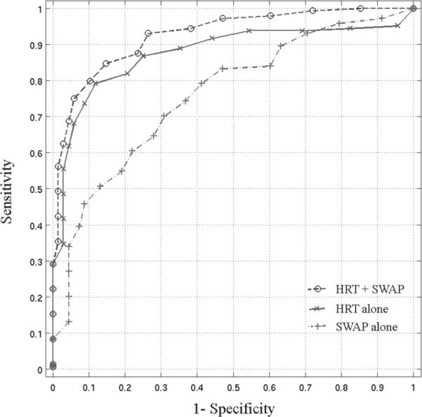
The ROC curves are presented for the RVM trained on the optimized HRT data alone (AUROC=0.878), SWAP thresholds plus age alone (AUROC=0.763) and on the combination HRT and SWAP thresholds plus age data (AUROC=0.925).
Grant Support
This research was supported by grants from the National Eye Institute, NIH EY08208 (PAS), NIH EY11008 (LMZ) and NIH EY13928 (MHG). Participant retention incentive grants in the form of glaucoma medication at no cost: Alcon Laboratories Inc, Allergan, Pfizer Inc, and SANTEN Inc.
Footnotes
Financial Disclosure: L. Racette, None; C.Y. Chiou, None; J. Hao, None; C. Bowd, Lace Elettronica (F); M.H. Goldbaum, None; L.M. Zangwill, Carl Zeiss Meditec, Inc. (F), Heidelberg Engineering (F), OptoVue (F), Allergan (F); T.-W. Lee, None; R.N. Weinreb, Carl Zeiss Meditec, Inc. (F, C), Heidelberg Engineering (F); P.A. Sample, Carl Zeiss Meditec, Inc. (F), Haag-Streit (F), Welch-Allyn (F)
REFERENCES
- 1.Weinreb RN, Khaw PT. Primary open-angle glaucoma. Lancet. 2004;363:1711–20. doi: 10.1016/S0140-6736(04)16257-0. [DOI] [PubMed] [Google Scholar]
- 2.Zangwill LM, Chan K, Bowd C, et al. Heidelberg retina tomograph measurements of the optic disc and parapapillary retina for detecting glaucoma analyzed by machine learning classifiers. Invest Ophthalmol Vis Sci. 2004;45:3144–51. doi: 10.1167/iovs.04-0202. [DOI] [PMC free article] [PubMed] [Google Scholar]
- 3.Miglior S, Casula M, Guareschi M, et al. Clinical ability of Heidelberg retinal tomograph examination to detect glaucomatous visual field changes. Ophthalmology. 2001;108:1621–7. doi: 10.1016/s0161-6420(01)00676-5. [DOI] [PubMed] [Google Scholar]
- 4.Ford BA, Artes PH, McCormick TA, et al. Comparison of data analysis tools for detection of glaucoma with the Heidelberg Retina Tomograph. Ophthalmology. 2003;110:1145–50. doi: 10.1016/S0161-6420(03)00230-6. [DOI] [PubMed] [Google Scholar]
- 5.Johnson CA, Adams AJ, Casson EJ, et al. Progression of early glaucomatous visual field loss as detected by blue-on-yellow and standard white-on-white automated perimetry. Arch Ophthalmol. 1993;111:651–6. doi: 10.1001/archopht.1993.01090050085035. [DOI] [PubMed] [Google Scholar]
- 6.Sample PA, Taylor JD, Martinez GA, et al. Short-wavelength color visual fields in glaucoma suspects at risk. Am J Ophthalmol. 1993;115:225–33. doi: 10.1016/s0002-9394(14)73928-5. [DOI] [PubMed] [Google Scholar]
- 7.Johnson CA, Samuels SJ. Screening for glaucomatous visual field loss with frequency-doubling perimetry. Invest Ophthalmol Vis Sci. 1997;38:413–25. [PubMed] [Google Scholar]
- 8.Racette L, Sample PA. Short-wavelength automated perimetry. Ophthalmol Clin North Am. 2003;16:227–36, vi-vii. doi: 10.1016/s0896-1549(03)00010-5. [DOI] [PubMed] [Google Scholar]
- 9.Shah NN, Bowd C, Medeiros FA, et al. Combining structural and functional testing for detection of glaucoma. Ophthalmology. 2006;113:1593–602. doi: 10.1016/j.ophtha.2006.06.004. [DOI] [PubMed] [Google Scholar]
- 10.Bowd C, Medeiros FA, Zhang Z, et al. Relevance vector machine and support vector machine classifier analysis of scanning laser polarimetry retinal nerve fiber layer measurements. Invest Ophthalmol Vis Sci. 2005;46:1322–9. doi: 10.1167/iovs.04-1122. [DOI] [PMC free article] [PubMed] [Google Scholar]
- 11.Bowd C, Zangwill LM, Medeiros FA, et al. Confocal scanning laser ophthalmoscopy classifiers and stereophotograph evaluation for prediction of visual field abnormalities in glaucoma-suspect eyes. Invest Ophthalmol Vis Sci. 2004;45:2255–62. doi: 10.1167/iovs.03-1087. [DOI] [PMC free article] [PubMed] [Google Scholar]
- 12.Goldbaum MH, Sample PA, Chan K, et al. Comparing machine learning classifiers for diagnosing glaucoma from standard automated perimetry. Invest Ophthalmol Vis Sci. 2002;43:162–9. [PubMed] [Google Scholar]
- 13.Goldbaum MH, Sample PA, Zhang Z, et al. Using unsupervised learning with independent component analysis to identify patterns of glaucomatous visual field defects. Invest Ophthalmol Vis Sci. 2005;46:3676–83. doi: 10.1167/iovs.04-1167. [DOI] [PMC free article] [PubMed] [Google Scholar]
- 14.Sample PA, Chan K, Boden C, et al. Using unsupervised learning with variational bayesian mixture of factor analysis to identify patterns of glaucomatous visual field defects. Invest Ophthalmol Vis Sci. 2004;45:2596–605. doi: 10.1167/iovs.03-0343. [DOI] [PMC free article] [PubMed] [Google Scholar]
- 15.Sample PA, Boden C, Zhang Z, et al. Unsupervised machine learning with independent component analysis to identify areas of progression in glaucomatous visual fields. Invest Ophthalmol Vis Sci. 2005;46:3684–92. doi: 10.1167/iovs.04-1168. [DOI] [PMC free article] [PubMed] [Google Scholar]
- 16.Mardin CY, Peters A, Horn F, et al. Improving glaucoma diagnosis by the combination of perimetry and HRT measurements. J Glaucoma. 2006;15:299–305. doi: 10.1097/01.ijg.0000212232.03664.ee. [DOI] [PubMed] [Google Scholar]
- 17.Caprioli J. Discrimination between normal and glaucomatous eyes. Invest Ophthalmol Vis Sci. 1992;33:153–9. [PubMed] [Google Scholar]
- 18.Brigatti L, Hoffman D, Caprioli J. Neural networks to identify glaucoma with structural and functional measurements. Am J Ophthalmol. 1996;121:511–21. doi: 10.1016/s0002-9394(14)75425-x. [DOI] [PubMed] [Google Scholar]
- 19.Bowd C, Hao J, Tavares IM, et al. Bayesian machine learning classifiers for combining structural and functional measurements to classify healthy and glaucomatous eyes. Invest Ophthalmol Vis Sci. 2008;49:945–53. doi: 10.1167/iovs.07-1083. [DOI] [PubMed] [Google Scholar]
- 20.Kass MA, Heuer DK, Higginbotham EJ, et al. The Ocular Hypertension Treatment Study: a randomized trial determines that topical ocular hypotensive medication delays or prevents the onset of primary open-angle glaucoma. Arch Ophthalmol. 2002;120:701–13. doi: 10.1001/archopht.120.6.701. discussion 829−30. [DOI] [PubMed] [Google Scholar]
- 21.Miglior S, Zeyen T, Pfeiffer N, et al. Results of the European Glaucoma Prevention Study. Ophthalmology. 2005;112:366–75. doi: 10.1016/j.ophtha.2004.11.030. [DOI] [PubMed] [Google Scholar]
- 22.Sample PA, Johnson CA, Haegerstrom-Portnoy G, et al. Optimum parameters for short-wavelength automated perimetry. J Glaucoma. 1996;5:375–83. [PubMed] [Google Scholar]
- 23.Sample PA, Medeiros FA, Racette L, et al. Identifying glaucomatous vision loss with visual-function-specific perimetry in the diagnostic innovations in glaucoma study. Invest Ophthalmol Vis Sci. 2006;47:3381–9. doi: 10.1167/iovs.05-1546. [DOI] [PubMed] [Google Scholar]
- 24.Medeiros FA, Zangwill LM, Bowd C, et al. Comparison of the GDx VCC scanning laser polarimeter, HRT II confocal scanning laser ophthalmoscope, and stratus OCT optical coherence tomograph for the detection of glaucoma. Arch Ophthalmol. 2004;122:827–37. doi: 10.1001/archopht.122.6.827. [DOI] [PubMed] [Google Scholar]
- 25.Dreher AW, Tso PC, Weinreb RN. Reproducibility of topographic measurements of the normal and glaucomatous optic nerve head with the laser tomographic scanner. Am J Ophthalmol. 1991;111:221–9. doi: 10.1016/s0002-9394(14)72263-9. [DOI] [PubMed] [Google Scholar]
- 26.Kruse FE, Burk RO, Volcker HE, et al. Reproducibility of topographic measurements of the optic nerve head with laser tomographic scanning. Ophthalmology. 1989;96:1320–4. doi: 10.1016/s0161-6420(89)32719-9. [DOI] [PubMed] [Google Scholar]
- 27.Wollstein G, Garway-Heath DF, Hitchings RA. Identification of early glaucoma cases with the scanning laser ophthalmoscope. Ophthalmology. 1998;105:1557–63. doi: 10.1016/S0161-6420(98)98047-2. [DOI] [PubMed] [Google Scholar]
- 28.Miglior S, Guareschi M, Albe E, et al. Detection of glaucomatous visual field changes using the Moorfields regression analysis of the Heidelberg retina tomograph. Am J Ophthalmol. 2003;136:26–33. doi: 10.1016/s0002-9394(03)00084-9. [DOI] [PubMed] [Google Scholar]
- 29.Strouthidis NG, White ET, Owen VM, et al. Factors affecting the test-retest variability of Heidelberg retina tomograph and Heidelberg retina tomograph II measurements. Br J Ophthalmol. 2005;89:1427–32. doi: 10.1136/bjo.2005.067298. [DOI] [PMC free article] [PubMed] [Google Scholar]
- 30.Mikelberg FS, Parfitt CM, Swindale NV, et al. Ability of the Heidelberg Retina Tomograph to detect early glaucomatous field loss. J Glaucoma. 1995;4:242–7. [PubMed] [Google Scholar]
- 31.DeLong ER, DeLong DM, Clarke-Pearson DL. Comparing the areas under two or more correlated receiver operating characteristic curves: a nonparametric approach. Biometrics. 1988;44:837–45. [PubMed] [Google Scholar]
- 32.Bishop CM, Tipping ME. In: Bayesian regression and classification, in Advances in learning theory: Methods, models and applicaitons. Suykens J, et al., editors. IOS Press; Amsterdam: 2003. pp. 267–85. [Google Scholar]
- 33.Medeiros FA, Ng D, Zangwill LM, et al. The effects of study design and spectrum bias on the evaluation of diagnostic accuracy of confocal scanning laser ophthalmoscopy in glaucoma. Invest Ophthalmol Vis Sci. 2007;48:214–22. doi: 10.1167/iovs.06-0618. [DOI] [PubMed] [Google Scholar]
- 34.Racette L, Medeiros FA, Bowd C, et al. The impact of the perimetric measurement scale, sample composition, and statistical method on the structure-function relationship in glaucoma. J Glaucoma. 2007;16:676–84. doi: 10.1097/IJG.0b013e31804d23c2. [DOI] [PubMed] [Google Scholar]
- 35.Ng M, Racette L, Pascual JP, et al. Comparing the Full Threshold and Swedish Interactive Thresholding Algorithms for Short-Wavelength Automated Perimetry. Invest Ophthalmol Vis Sci. 2008 doi: 10.1167/iovs.08-2718. [DOI] [PMC free article] [PubMed] [Google Scholar]