Abstract
Many experiments have investigated visual search for simple stimuli like colored bars or alphanumeric characters. When eye movements are not a limiting factor, these tasks tend to produce roughly linear functions relating reaction time (RT) to the number of items in the display (set size). The slopes of the RT × set size functions for different searches fall on a continuum from highly efficient (slopes near zero) to inefficient (slopes > 25-30 msec/item). Many theories of search can produce the correct pattern of mean RTs. Producing the correct RT distributions is more difficult. In order to guide future modeling, we have collected a very large data set (about 112,000 trials) on three tasks: an efficient color feature search, an inefficient search for a 2 among 5s, and an intermediate color × orientation conjunction search. The RT distributions have interesting properties. For example, target absent distributions overlap target present more than would be expected if the decision to end search were based on a simple elapsed time threshold. Other qualitative properties of the RT distributions falsify some classes of model. For example, normalized RT distributions do not change shape as set size changes as a standard self-terminating model predicts that they should.
Visual search has been one of the leading paradigms in the study of visual attention for more than a generation. In part this is because laboratory visual search is an abstraction of very real tasks we perform every day. In the world, we search for the can opener in the kitchen drawer or the cat in the living room. In the lab, we search for the T among Ls or the red vertical line among green verticals and red horizontals. In return for the artificiality of standard lab search tasks, we gain the ability to tightly control the stimuli and to run the same search for hundreds of trials. By measuring reaction time (RT) and/or accuracy, we have been able to uncover regularities in search behavior (reviewed in Pashler, 1998; Sanders & Donk, 1996; Wolfe, 1998; Wolfe, 1998; Wolfe & Horowitz 2007) and to build models on those regularities (e.g. Cave, 1999; Grossberg, Mingolla, & Ross, 1994; Hamker, 2004; Hoffman, 1979; Humphreys & Muller, 1993; Pomplun, Reingold, & Shen, 2002; Thornton & Gilden, 2007; Treisman & Gelade, 1980; Tsotsos et al., 1995; Verghese, 2001; Wolfe, 1994).
The bulk of work on visual search has used mean RT or accuracy measures. Here we will focus on tasks where the stimulus is visible until response and where RT is the primary measure of interest. Mean (or median) RT data are very useful, with the standard measure for search efficiency being the slope of a linear function relating RT to the number of items in the display (set size). Patterns of RT × set size functions have been used to argue for various models of search. For example, slopes of target-absent trials tend to be about twice those of target-present trials. This would be predicted if observers searched serially through an average of half the items in order to find the target on target-present trials and then searched exhaustively through all items to confirm that a target was absent on absent trials (Sternberg, 1966; Treisman & Gelade, 1980). Unfortunately, these results from mean RT have been less constraining than might be hoped. Continuing with the example, it has been shown that various parallel models can be induced to produce the 2:1 slope ratio (J. Palmer, 1995; Townsend, 1971; Townsend & Wenger, 2004). Moreover, it is unlikely that items are sampled exhaustively and without replacement on target absent trials (Horowitz & Wolfe, 1998; Horowitz & Wolfe, 2001) and, as it happens, the real absent/present slope ratio is probably significantly greater than the predicted 2.0 (Wolfe, 1998).
The purpose of this paper is to bring new constraints on theory from RT data by looking at the distributions of RT as well as measures of their central tendency. Though only a limited amount of prior work has been done, there are some notable examples of work on RT distributions in search. Hockley (1984) compared visual search to memory search and argued that increases in mean RT with set size were driven by different parameters of the functions that capture RT distribution shape in the two tasks. Cousineau & Shiffrin (2004) used analyses of distributions to test the standard serial self-terminating search model. They found evidence for serial search, but also showed that termination rules vary from observer to observer. Sung (2008) looked at RT distributions for displays of set size of four in an effort to distinguish parallel from serial mechanisms.
In the present work, our particular interest was to collect a body of data that would permit us to look at RT distributions in the sorts of tasks that have been important in the literature on mean RT in search. Such a data set has not existed because it requires a large number of trials from a reasonable number of observers.
To obtain this data set, we collected 1000 trials from nine or ten observers at each of four set sizes for three of the most popular laboratory search tasks (4000 trials per observer per task, approximately 112,000 RTs in total). This allows us to present the most robust RT × set size functions yet published for these tasks. More importantly, we have enough trials in each cell of the design to create meaningful characterizations of the RT distributions. In this paper, we will discuss the important qualitative properties of these distributions. It is also possible to look at the data more quantitatively. For example, like Hockley (1984), one could fit different functions to the data and base conclusions on the goodness of fit and the values of the fitting parameters. We do this elsewhere (E. M. Palmer, Horowitz , Torralba, & Wolfe, 2009).
Looking at the distributions without a commitment to specific underlying functions, their most striking aspect is the similarity in their shapes across set sizes, and for the most part, across tasks and target presence/absence. We will show how this constrains models of search by discussing how the pattern of results eliminates various classes of model. On the assumption that it is best to throw stones at one's own glass house first, we will show how these results raise problems for current versions of models like our own Guided Search (Wolfe, 2007) but we note that these data challenge most models.
Methods
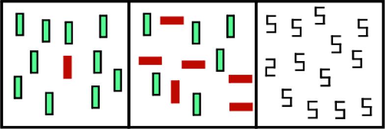
We ran three standard visual search tasks, intended to span a range of processing difficulties. Illustrations of target present trials are shown in Figure 1. Task 1 tested participants on a simple feature search for a red vertical rectangle among green vertical rectangles. This task typically yields RT × set size search slopes near zero. Task 2 was a conjunction search task for a red vertical rectangle among green vertical and red horizontal rectangles. This task typically yields RT × set size functions with a moderate slope of around 10 ms/item. Finally, in Task 3 observers searched for a digital “2” among digital “5”s (‘2 vs. 5’ ). These targets and distractors are composed of the same horizontal and vertical components, but in different configurations. This “spatial configuration” task typically yields RT × set size functions with steep slopes of 30 or more ms/item. Such tasks are often called “serial search tasks”. While there is evidence supporting serial deployment of attention in such tasks (Bricolo, Gianesini, Fanini, Bundesen, & Chelazzi, 2002; Kwak, Dagenbach, & Egeth, 1991; Woodman & Luck, 2003) calling the task “serial” is a theoretical claim so we will instead refer to this as a “spatial configuration task” (Wolfe, 1998). Similarly, we will not refer to slope values as “parallel” and “serial”. Again, we will avoid the ideological commitment by calling slopes near zero “efficient” and slopes of greater than about 30 msec/item “inefficient”. Of course, it is possible to devise searches that produce slopes far greater than 30 msec/item. For example, a task that forces fixation on each item before it can be identified will have a slope of at least 125-250 msec/item (Findlay, Brown, & Gilchrist, 2001; Porter, Troscianko, & Gilchrist, 2007). However, here we are working with stimuli that can be easily identified outside of the fovea.
Figure 1.
Search displays corresponding to the three tasks. Experimental displays were presented on a black background. On the left, participants searched for a red (solid) vertical rectangle among green (outline) vertical rectangles (Feature search). In the middle, participants searched for a red vertical rectangle among green vertical and red horizontal rectangles (Conjunction Search). On the right, participants searched for a digital 2 among digital 5s (Spatial Configuration Search).
These three tasks were chosen because they span a range of search difficulty that has been of theoretical interest for many years. One way to interpret the variation of slopes in this range is to propose that it reflects a variation in the amount of available ‘guidance,’ (roughly, the strength of the signal attracting deployments of attention towards the target item, Wolfe, Cave, & Franzel, 1989). In feature search, color guides attention to the target the first time, almost every time; consequently distractors get little or no attention and search slopes are near zero. In spatial configuration search, no basic attribute can guide attention so selection mechanisms must sample randomly from the display at a rate that produces target-present slopes of about 30 msec/item. In conjunction search, no single feature can direct attention straight to the target but the combination of relevant color and orientation provide enough guidance to bias selection imperfectly toward the target item. The result is a reasonably efficient slope of around 10 msec/item. Conceptualizing visual search as a series of prioritized deployments of attention is not the only approach to understanding search. Many alternative accounts can describe the continuum of search efficiencies. These include models grounded in a signal detection (Cameron, Tai, Eckstein, & Carrasco, 2004; Verghese, 2001; Verghese & Nakayama, 1994) or biased-choice framework (Bundesen, 1990, 1998). By using these tasks we have collected a data set that should be useful to modelers with a range of approaches. Of course, the choice of these three tasks will not allow all theoretically interesting issues to be addressed. For example, in the present work, the target is fixed across all trials in a block. There might be interesting differences between these tasks and odd-man-out tasks where targets change from trial to trial. Similarly, one would like to have data on hard feature searches that produce inefficient search, several different conjunction searches, and so forth. Thus, the present selection of tasks can be seen as a start of what could be a far larger project.
Participants
Thirty observers between the ages of 18-55 (all but one younger than 30) participated in the three tasks. One observer completed both the conjunction search and spatial configuration search tasks. Another observer participated in both the feature search and spatial configuration search tasks, but was subsequently removed from the data set for failing to follow experimental instructions and protocol in several other studies. The excluded observer's data were qualitatively and quantitatively very different from the other nine observers in each of the two tasks. Consequently, nine observers were analyzed in the feature and spatial configuration search tasks, while ten observers were analyzed in the conjunction search task.
Each observer passed the Ishihara color test and had 20/25 vision or better (with correction, if necessary). All observers gave informed consent before participating and were paid $8 per hour for approximately four to six hours of testing time.
Materials
Stimuli were presented on an Apple Macintosh G4 450 MHz computer driving a 20” (diagonal) CRT monitor at a resolution of 1024 × 768 pixels. Responses were gathered with an Apple Macintosh USB keyboard. The experiment was controlled using Matlab 5.2.1 and the Psychophysics Toolbox (Brainard, 1997; Pelli, 1997).
At the viewing distance of 57.4 cm, the display area was a square measuring 22.5 degrees visual angle (°) on a side. This region was divided into an invisible 5 × 5 array of cells, with each cell subtending 4.5° × 4.5°. If the cell contained a display item, it was positioned at a random location within the cell.
Procedure
Observers were seated at the computer in a quiet, darkened room. A white fixation cross (0.7° × 0.7°) appeared in the center of the screen throughout the experiment. Observers were instructed to keep their eyes focused on this cross, but we did not monitor eye movements. In this class of task, RT data look similar with and without enforced fixation (Zelinsky & Sheinberg, 1997). At the beginning of each trial, a short tone was played. After an interval of 500 ms, the search display appeared and remained visible until the observer pressed a key to indicate target-present or target-absent. Participants were instructed to respond as quickly and accurately as possible, and were shown a feedback display for 500 ms after each trial, reporting whether they responded correctly or not. The inter-trial interval was 1000 ms, and participants could pause the experiment at any time by pressing the space bar.
Observers completed 30 practice trials at the beginning of each block and were tested on 12 blocks of 300 experimental trials and one block of 400 experimental trials, for a total of 4000 experimental trials and 390 practice trials. Practice trials were discarded from the analyses. On each trial, both the presence or absence of the target and the set size of the display were chosen randomly, with a 50% probability of either a target-absent or target-present trial and a 25% probability of a display with 3, 6, 12, or 18 items.
Stimuli
Task 1: Feature Search
Search items were vertical bars, subtending 1.0° × 3.5°. The target item was always a red vertical bar (CIE: x = .630, y = .375, luminance = 4.5 cd/m2), while distractors were green vertical bars (CIE: x = .300, y = .600, luminance = 13.0 cd/m2). All displays were shown on a black background (CIE: x=.322, y=.200, luminance=.02 cd/m2).
Task 2: Conjunction Search
Search items consisted of horizontal and vertical bars, subtending 3.5° × 1.0° or 1.0° × 3.5°, respectively. The target item was a red vertical bar, while distractors were red horizontal bars and green vertical bars. The red and green items had the same luminance profiles as the stimuli used in Task 1. All displays were shown on a black background with the same luminance profile as in Task 1.
Task 3: Spatial Configuration Search
Search items were digital 2s and 5s, each subtending 1.5° × 2.7°. The target item was a white digital 2 (CIE: x=.300, y=.350, luminance=14.7 cd/m2), while distractors were white digital 5s, both presented on a black background with the same luminance profile as in Task 1.
Data Analyses and Procedures
Assuming that unreasonably fast RTs represented anticipations and unreasonably slow RTs represented attentional lapses, we excluded all trials with RTs < 200 ms or > 4000 ms for the feature and conjunction search tasks and RTs < 200 ms or > 8000 ms in the spatial configuration search task. A total of just 80 trials or .07% of the entire data set for all observers across all three tasks were removed by this method. Given the large sample sizes of our data and the relatively few RTs that were excluded, we can expect that truncation of the RT data set in this manner will have little or no effect on our distributional analyses. Indeed, in our work fitting these data to specific distributions we find very modest (<3%) differences in the goodness-of-fit with and without the excluded trials. Note that this is very different from the practice of deleting, for example, all RTs more than 3 standard deviations from the mean. The full data set is posted at our website, so interested parties can analyze the data with any desired exclusion rule.
Results
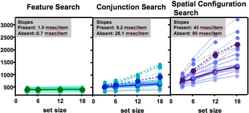
Figure 2 shows RT from correct target present and absent trials. The figure shows data for each individual (lighter lines) and the average data (darker). With each mean RT data point representing about 500 trials, this is probably the most robust published data set for these standard search tasks. The full data set is downloadable at http://search.bwh.harvard.edu/new/data_set.html.
Figure 2.
RT × set size data: Lighter lines show data for individual observers. Darker lines and data points show mean data. Solid lines show target present results. Dashed lines show target absent. Since all tasks are plotted on the same y-axis, feature search present and absent data overlap nearly completely.
The mean RT data confirm the findings of many studies. Feature search is extremely efficient. Search for a 2 among 5s is inefficient. A color orientation conjunction search is quite efficient though clearly not as efficient as a feature search. For the conjunction and ‘2 vs. 5’ tasks, where the slopes are above zero, the slope ratios are somewhat greater than 2 msec/item (Wolfe, 1998), though the deviation from 2.0 msec/item is not statistically reliable (Conjunction: t(9)=1.7, p=0.12; ‘2 vs. 5’ : t(8)=1.6, p=.15). Variability between observers is greater on the target absent trials than on target present trials. This presumably reflects differences in decision criteria (Cousineau & Shiffrin, 2004).
Error Analyses
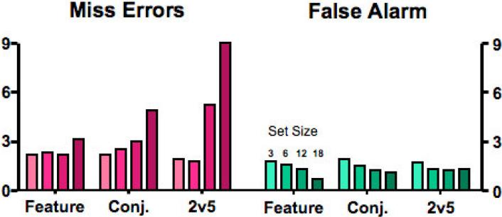
Figure 3 shows average error rates for each task by set size. As is typical in these tasks, there were more miss errors than false alarms (a ratio of 2.9:1). Miss error rates increased with set size and with task difficulty (i.e., RT × set size slope). False alarm rates were relatively constant or slightly declining across tasks. The apparent decline in false alarm rates with set size is reliable for feature search (t(8)=5.23, p=0.0008) marginal for conjunction (t(9)=2.22, p=0.05), and not significant for the ‘2 vs. 5’ task (t(8)=0.58, p=0.58). Such a decline, paired with the increase in miss errors, would be consistent with a criterion shift toward a more conservative position at higher set sizes. In general, the error rates were somewhat lower than what is typically seen in these tasks, perhaps because of observers’ extensive practice. Note that the most substantial error rates are the 5.2% and 9.3% miss error rates for the larger set sizes in the ‘2 vs. 5’ task. This may reflect a type of speed-accuracy tradeoff in which trials, which would have produced the longest RTs in this study were aborted by the observer, producing faster mean RTs at the cost of higher errors. The possibility that this truncation may affect the RT distributions will be considered later.
Figure 3.
Mean error rates for each set size and for each task. The four bars for each task represent the four set sizes. Thus, for example, it can be seen that error rates are highest for spatial configuration miss errors and that these rise with set size.
RT Distributions
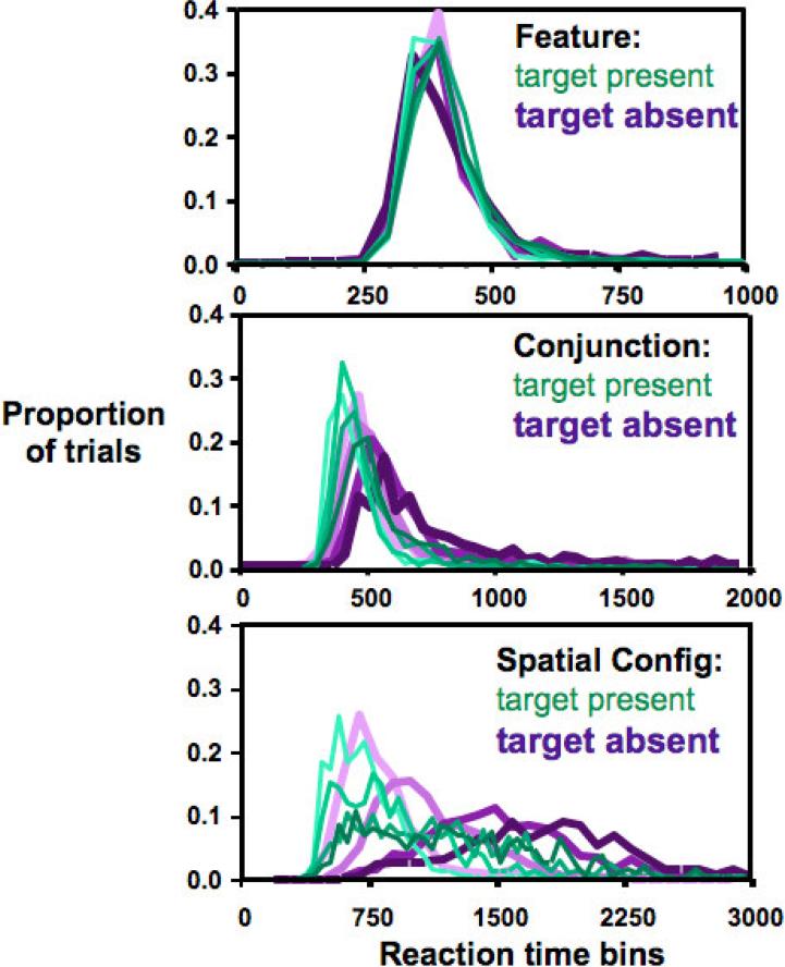
The primary purpose of this paper is to examine the RT distributions for these standard search tasks. We put our observers through the pleasure of 4000 trials per task in order to have 500 trials (minus error trials) with which to create distributions for target present and target absent trials at each set size for each task. We tabulated the RTs in 50 msec-wide bins to create histograms. Data for representative observers are shown in Figure 4. The mean RT data for these observers fall close to the grand mean RTs of the group.
Figure 4.
RT distributions for one observer from each of the three tasks (different observers for each task). Each distribution represents one set size for target present (thin, green) or target absent (fat, purple) trials. Set size is coded by lightness from the lightest lines, set size 3, through set sizes 6 and 12 to the darkest, set size 18. Note the different X-axes for the different tasks.
These data are similar to those for the other observers. One obvious feature of these plots is that the RT distributions shift to the right as the mean RT increases. Thus, for the conjunction and ‘2 vs. 5’ tasks, target absent distributions are generally to the right of target present and distributions progress rightward as set size increases. Variance tracks mean RT. Thus, the longer search for a 2 among 5s produces broader, shallower distributions than the feature search. All of the distributions are positively skewed, a characteristic of RT distributions in general (Luce, 1986; Van Zandt, 2002).
The best way to describe the shape of these functions is less obvious. Many functions have the appropriate positively skewed shape if properly parameterized (e.g. ex-Gaussian, ex-Wald, Gamma, and Weibull). Since there have been efforts to map the parameters of different functions onto different psychological processes, we have fit the present data to a number of these functions (E. M. Palmer, Horowitz , Torralba et al., 2009). However, one could argue that this is a problematic approach to modeling RT distributions in visual search because empirical distributions are likely to be complex mixtures of several components. As a generic model of the variability in search, we might assume that there are, at least, three components: initial visual processing, the search itself, and response generation. The response/motor component produces a positively skewed distribution (Van Zandt, 2002) and it is possible to separately influence these stages in search tasks (Wolfe, Oliva, Horowitz, Butcher, & Bompas, 2002). Thus, while the formal analysis of the shapes of the distributions may be valuable, in this paper, we will focus on the qualitative attributes that do not require a commitment to any particular generating function.
Implications for models of search termination
Understanding how search is terminated on target absent trials has been a long-standing problem in visual search (Chun & Wolfe, 1996; Cousineau & Shiffrin, 2004; Hong, 2005). The distribution data can eliminate a range of “straw man” models and put strong constraints on more plausible candidates. Consider a straw man version of a classic, serial, self-terminating model of search (e.g. some simple version of Feature Integration Theory, Treisman & Gelade, 1980). The distribution of times required to find a target when the target is present should be essentially rectangular. If you have, say, ten items, then there is a 10% chance of finding the target on your first selection of an item, 10% on the second, and so on. Target absent responses would occur after all ten items were rejected. Thus, in the most simple-minded version, all target-absent RTs would be identical for a given set size. A slightly less simple-minded version would predict that the variance of the absent trial RTs should be lower than the variance of the present trial RTs.
Clearly, the data are at odds with these predictions. The distribution of target present RTs is nothing like rectangular and, as has been noted elsewhere (Ward & McClelland, 1989), the variance of the absent trials is greater than that of the target present trials. Moreover, the shapes of the present and absent distributions look rather similar where this account would predict that they would be completely different.
We can propose, and then reject, a less artificial account of the termination of target-absent trials. A generic account of search termination might predict that observers learn something about the distribution of RTs for successful searches on target present trials and then use this knowledge to develop a quitting threshold for absent trials. The observer's implicit logic might be something like this: “If I have searched a display of N items for M msec, there is only a P% chance that I have missed a target. Once P is below some threshold, I can safely abandon this search with a ’target-absent‘ response.” Analyzing sequences of search RTs yields evidence for an adaptive mechanism of this sort: RTs speed up after successful responses and slow after errors (Chun & Wolfe, 1996).
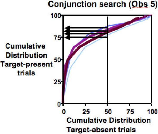
This account would predict that the median absent RT should lie relatively far out on the target present distribution. The exact position would depend on the model and the error rate for the observer but, to a first approximation, one would imagine that the median absent RT should lie around the 95th percentile on the target present distribution if the observer was willing to tolerate about 5% miss errors. Looking at the data in Figure 4, the distributions seem to overlap more than this prediction would allow. This point is illustrated more quantitatively in Figure 5.
Figure 5.
Target-present cumulative distribution function plotted against target absent for the conjunction data of Figure 4. Vertical line represents the median of the absent distributions. Horizontal arrows show where those medians fall on the target present distribution. Each line represents a different set size from thin, light blue (3) to fat, dark red (18).
For illustrative purposes, Figure 5 shows the conjunction search data for the sample observer of Figure 4. The median target absent RTs for this observer in the conjunction task lie between the 75th and 85th percentiles on the target present distribution, meaning that half of the absent RTs take less time than 15-25% of the present RTs. Table 1 shows these data summarized across all observers for the conjunction condition.
Table 1. Location of the median target-absent RT on the target-present RT distribution.
The values in this table are obtained by finding the percentile on the target present distribution that corresponds to the median target absent RT for the conjunction task. Mean percentile, standard deviations, and confidence intervals are derived from the data of all observers. Average miss errors are tabulated in the bottom row.
| Set size 3 | Set size 6 | Set size 12 | Set size 18 | |
|---|---|---|---|---|
| Mean percentile | 70.05 | 76.83 | 82.03 | 82.67 |
| Std. Deviation | 9.928 | 7.448 | 7.174 | 8.863 |
| Std. Error | 3.139 | 2.355 | 2.269 | 2.803 |
| Lower 95% CI of mean | 62.95 | 71.50 | 76.90 | 76.33 |
| Upper 95% CI of mean | 77.15 | 82.16 | 87.16 | 89.01 |
| Miss Errors | 2.2% | 2.5% | 3.0% | 4.9% |
Results are similar for the other two tasks. It is clear that placing a quitting criterion at the position of the median absent RT would predict error rates much higher than the 2-5% errors produced by our observers in this condition (bottom row of table). Whatever rule is being used to terminate target absent searches, it is not simply to wait until there is only a 2-5% chance of a longer target present RT. One possibility is that the post-decision component of target present responses takes longer than the post-decision component of target absent. Hypothetically, a decision to respond, “yes, I see the target”, might invoke additional processes (perhaps the planning of a saccade) while the decision to respond “no” would not. The result would be that the final target-present RT distribution would slide a bit closer to the target absent distribution, producing the effect seen here. Alternatively, the decision to quit might be based on an internal signal; for instance, some count of the number of deployments of attention, rather than on elapsed time. These particular solutions to the problem are, of course, entirely ad hoc, but the example serves to illustrate how examination of distributions can shape theory.
The shapes of the distributions
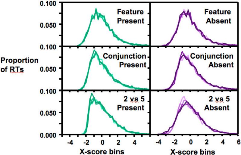
As a general rule, we run multiple observers in experiments of this sort in order to allow us to average or otherwise aggregate the data across observers. With RT distributions, however, we cannot simply average across observers, since differences in the means and spread of the distributions for different observers would distort the shape of the average distribution. We would like a way to combine and/or compare distributions. One solution is to normalize the distributions, but the standard z-score normalization, subtracting each value from the mean and dividing by the standard deviation, would be inappropriate with clearly skewed distributions. Instead, we have developed a non-parametric normalization procedure that we have named the “x-score transform” (E. M. Palmer, Horowitz , & Wolfe, 2009), which linearly scales distributions via quantile alignment. The x-score transform aligns the 25th and 75th percentiles of a distribution to any two arbitrary values (e.g., −1 and +1, respectively). This removes linear scaling differences in distributions while preserving non-linear properties such as the skew and kurtosis. Unlike a z-score, it does not assume symmetry around the mean, thus the peak of the distribution need not be at zero after x-transformation. We have shown that this process is capable of distinguishing between, for example, gamma and normal distributions with the same mean and standard deviation (E. M. Palmer, Horowitz , & Wolfe, 2009).
Figure 6 shows the results of this non-parametric normalization on the present data set. These are x-score distributions for each task at each set size for correct present and absent trials, combined across observers. Each distribution was first x-scored so that the 25th and 75th percentile RT fell at -1 and +1, respectively, and then the x-scored distributions were pooled across subjects before plotting.
Figure 6.
Group RT distributions normalized by the X-score method
The most striking observation is that, once rescaled, all of these distributions look very similar. Within a condition, the set size variable disappears. Target present and target absent distributions are very similar, with the possible exception of the ‘2 vs. 5’ task. In the paper discussing the x-score method in detail (E. M. Palmer, Horowitz , & Wolfe, 2009), we describe quantitative methods for determining if x-scored distributions are statistically different from each other. Here, we continue to focus on the more general, qualitative constraints on models that are implied by the similarity of the normalized functions. For example, a model that predicts non-linear shape differences for target present and target absent distributions will fail for feature and conjunction search. However, the ‘‘2 vs. 5’ ’ task does appear to produce a different shape for present and absent trials (note that the present trial distributions rise more steeply on the left side than the absent distributions).
This disparity might reflect a difference between the mechanisms of inefficient 2v5 searches and more efficient feature and conjunction searches. Alternatively, the difference might reflect the effects of errors. It may be hard to see in the lower right panel of Figure 6, but the distributions for the larger set sizes (darker) have a shallower rise on the left side than the two smaller set sizes (lighter). Indeed, the x-score distributions for ‘2 vs. 5’ target absent, set sizes 12 and 18, are each reliably different than both set sizes 3 and 6 according to the Kolmogorov-Smirnov test, each p < .0083 (alpha of .05 corrected for six comparisons). Recall from Figure 3 that set sizes 12 and 18 in the ‘2 vs. 5’ task produced markedly higher miss error rates, which may have caused the differences in distribution shape. Modeling speed-accuracy tradeoffs is tricky (McElree & Carrasco, 1999; Ruthruff, 1996) and even correcting mean RTs for the effects of errors is more an art than a science. This question might be addressed by a future experiment in which several RT distributions were collected from the same observers while error rates were manipulated by use of different reward structures, for example.
With the exception of those ‘2 vs. 5’ absent distributions, there is very little effect of varying set size on the shape of the RT distributions. This is theoretically interesting. Consider the very generic model discussed earlier. The measured RT will be the sum of three components: initial visual processing, the search, and a motor/decision stage (two components if one believes that the search and the visual processing are concurrent). Each component contributes a time that is distributed in some fashion. Thus, the final RT distribution is a mixture distribution. As set size increases, the search component increases its mean and variance. Presumably, the motor/decision component does not scale with set size. Thus, the mixture distribution is changing but it is doing so without changing shape. This implies that if the search component scales with set size, it must do so in a linear fashion that is removed by x-scoring.
To see how this could falsify a model, we simulated a version of a standard, serial, self-terminating search. For this simulation, we chose parameters that would roughly replicate the mean RT data of the spatial configuration, ‘2 vs. 5’ task. Thus, in the simulation, attention was deployed to an item on average every 98 msec. The deployment times were drawn from a gamma distribution with shape parameter = 7 and scale = 14, in order to give them a positively skewed distribution. On target absent trials, the simulated number of attentional deployments was equal to the set size. On target present trials, the number of deployments was drawn at random from the integers between 1 and the set size, as it would be in a serial, self-terminating search with memory for rejected distractors (Todd S. Horowitz, 2006). The simulated RT was the sum of the times for each deployment plus a motor/decision component that was gamma distributed with shape parameter = 7 and scale = 14, adding an average of 200 msec to each RT. The choice of specific parameters, the choice of a gamma distribution, and the choice of a search model with full memory are all arbitrary choices for the purposes of illustration. The mean RTs, produced by simulation, have a target present slope of 49 msec/item and a target absent slope of 98 msec/item, close to the ‘2 vs. 5’ results shown in Figure 2.
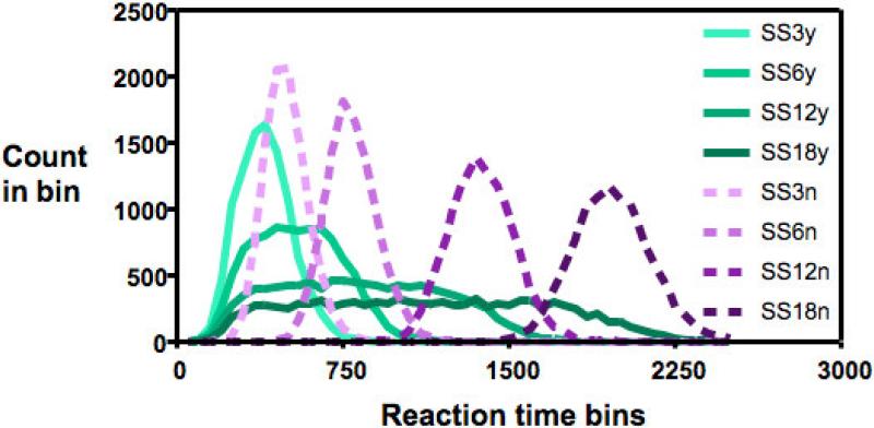
The value of RT distributions in evaluating models can be seen if we plot the distributions for the simulated model.
Examining Figure 7, it is clear that the distributions are qualitatively different from the distributions in Figure 4. In particular, the target-absent distributions look nothing like the real distributions. Again, note that we are not making any claims about this specific simulation beyond noting that it produces roughly the correct mean RTs. We use this example to show how the distributions can be used to reject a model that an analysis based on simple mean RT might have accepted (Cousineau & Shiffrin, 2004). In fact, we observe with some regret that the model simulated here is quite close to the proposals of Guided Search 2.0 for this condition (Wolfe, 1994). It is possible that other classes of model (e.g. a parallel model like Palmer, 1995, or a race model like Bundesen, 1998) might fare better. It is our hope that proponents of other types of model will test them against this data set.
Figure 7.
RT distributions for simulated serial, self-terminating search. Solid lines represent target present distributions; dashed, target absent. Lighter lines represent smaller set sizes.
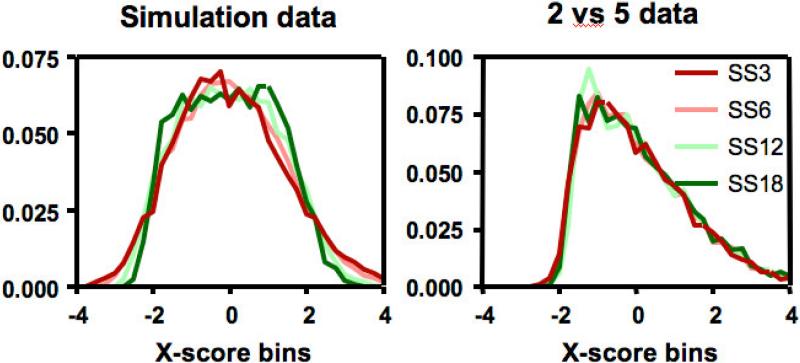
Looking at Figures 4 and 7, we might conclude that, while our toy model fails spectacularly for target absent trials, it does not do too badly for target present trials. Here it is useful to normalize the data using the x-score method as shown above, in Figure 6. Figure 8 shows the result of x-score normalization for the target present trials of the simulation.
Figure 8.
X-score transformed distributions for the target present trials in the simulation (left) and the ‘2 vs. 5’ task (right).
Here we see that the shapes of the simulated target present distributions become more rectangular with increasing set size, as the search component of the mixture comes to dominate the perceptual and decision/motor components. The scale of the figure is magnified to make this point clear. We re-plot the relevant data from Figure 6 at the same magnification in order to demonstrate that there is no such variation in the shape of the distributions in the real data.
Conclusion
To summarize, we have collected the most extensive data set on three of the standard tasks in the visual search literature. We have posted the data on our website (http://search.bwh.harvard.edu/new/data_set.html) and we encourage others to mine it for new information about search. Looking at the usual mean RT data, we have replicated the standard findings. However, our goal has been to show how the RT distributions can be used to provide new information about the mechanisms of search. We have described three examples. First, target present and target absent distributions overlap more than one might expect. Observers can terminate absent trials successfully with median absent RTs that are faster than 15-25% of the target present RTs. Second, at least for feature and conjunction search, the normalized distributions for present and absent trials are very similar. Finally, under most conditions, set size has no observable impact on the x-score normalized distributions. The challenge for modelers of human search behavior will be to propose models that can meet these constraints. The published versions of our Guided Search model would not succeed. Of course, we are working on the next generation of the model that takes these new findings into account. We will leave it to proponents of other models to determine how well those models can reproduce these findings.
Acknowledgments
We gratefully acknowledge support of this research from Ruth L. Kirschstein NRSA Grant EY016632 to EMP, and AFOSR Grant FA9550-06-1-0392 and NIH MH056020 to JMW.
Footnotes
Publisher's Disclaimer: This is a PDF file of an unedited manuscript that has been accepted for publication. As a service to our customers we are providing this early version of the manuscript. The manuscript will undergo copyediting, typesetting, and review of the resulting proof before it is published in its final citable form. Please note that during the production process errors may be discovered which could affect the content, and all legal disclaimers that apply to the journal pertain.
Contributor Information
Jeremy M Wolfe, Brigham & Women's Hospital and Harvard Medical School.
Evan M Palmer, Wichita State University.
Todd S Horowitz, Brigham & Women's Hospital and Harvard Medical School.
REFERENCES
- Brainard DH. The Psychophysics Toolbox. Spatial Vision. 1997;10:443–446. [PubMed] [Google Scholar]
- Bricolo E, Gianesini T, Fanini A, Bundesen C, Chelazzi L. Serial attention mechanisms in visual search: a direct behavioral demonstration. J Cogn Neurosci. 2002;14(7):980–993. doi: 10.1162/089892902320474454. [DOI] [PubMed] [Google Scholar]
- Bundesen C. A theory of visual attention. Psychol Rev. 1990;97(4):523–547. doi: 10.1037/0033-295x.97.4.523. [DOI] [PubMed] [Google Scholar]
- Bundesen C. A computational theory of visual attention. Philos Trans R Soc Lond B Biol Sci. 1998;353(1373):1271–1281. doi: 10.1098/rstb.1998.0282. [DOI] [PMC free article] [PubMed] [Google Scholar]
- Cameron EL, Tai JC, Eckstein MP, Carrasco M. Signal detection theory applied to three visual search tasks--identification, yes/no detection and localization. Spat Vis. 2004;17(4-5):295–325. doi: 10.1163/1568568041920212. [DOI] [PubMed] [Google Scholar]
- Cave K. The FeatureGate model of visual selection. Psychol Res. 1999;62(2-3):182–194. doi: 10.1007/s004260050050. [DOI] [PubMed] [Google Scholar]
- Chun MM, Wolfe JM. Just say no: How are visual searches terminated when there is no target present? Cognitive Psychology. 1996;30:39–78. doi: 10.1006/cogp.1996.0002. [DOI] [PubMed] [Google Scholar]
- Cousineau D, Shiffrin RM. Termination of a visual search with large display size effects. Spat Vis. 2004;17(4-5):327–352. doi: 10.1163/1568568041920104. [DOI] [PubMed] [Google Scholar]
- Findlay JM, Brown V, Gilchrist ID. Saccade target selection in visual search: the effect of information from the previous fixation. Vision Res. 2001;41(1):87–95. doi: 10.1016/s0042-6989(00)00236-4. [DOI] [PubMed] [Google Scholar]
- Grossberg S, Mingolla E, Ross WD. A neural theory of attentive visual search: Interactions of boundary, surface, spatial and object representations. Psychological Review. 1994;101(3):470–489. doi: 10.1037/0033-295x.101.3.470. [DOI] [PubMed] [Google Scholar]
- Hamker FH. A dynamic model of how feature cues guide spatial attention. Vision Res. 2004;44(5):501–521. doi: 10.1016/j.visres.2003.09.033. [DOI] [PubMed] [Google Scholar]
- Hockley WE. Analysis of response time distributions in the study of cognitive processes. Journal of Experimental Psychology: Learning, Memory, & Cognition. 1984;10(4):598–615. [Google Scholar]
- Hoffman JE. A two-stage model of visual search. Perception and Psychophysics. 1979;25:319–327. doi: 10.3758/bf03198811. [DOI] [PubMed] [Google Scholar]
- Hong S-K. Human stopping strategies in multiple-target search. International Journal of Industrial Ergonomics. 2005;35:1–12. [Google Scholar]
- Horowitz TS. Revisiting the variable memory model of visual search. Visual Cognition. 2006;19(4-8):668–684. [Google Scholar]
- Horowitz TS, Wolfe JM. Visual search has no memory. Nature. 1998;394:575–577. doi: 10.1038/29068. Aug 6. [DOI] [PubMed] [Google Scholar]
- Horowitz TS, Wolfe JM. Search for multiple targets: Remember the targets, forget the search. Perception and Psychophysics. 2001;63(2):272–285. doi: 10.3758/bf03194468. [DOI] [PubMed] [Google Scholar]
- Humphreys GW, Muller H. SEarch via Recursive Rejection (SERR): A connectionist model of visual search. Cognitive Psychology. 1993;25:43–110. [Google Scholar]
- Kwak H, Dagenbach D, Egeth H. Further evidence for a time-independent shift of the focus of attention. Perception & Psychophysics. 1991;49(5):473–480. doi: 10.3758/bf03212181. [DOI] [PubMed] [Google Scholar]
- Luce RD. Response Times. Oxford U. Press; New York: 1986. [Google Scholar]
- McElree B, Carrasco M. The temporal dynamics of visual search: evidence for parallel processing in feature and conjunction searches. J Exp Psychol Hum Percept Perform. 1999;25(6):1517–1539. doi: 10.1037//0096-1523.25.6.1517. [DOI] [PMC free article] [PubMed] [Google Scholar]
- Palmer EM, Horowitz TS, Torralba A, Wolfe JM. What is the shape of response time distributions in visual search tasks? J. Exp. Psychol: Human Perception and Performance. 2009 doi: 10.1037/a0020747. in revision. [DOI] [PMC free article] [PubMed] [Google Scholar]
- Palmer EM, Horowitz TS, Wolfe JM. The x-score transform: A non-parametric technique for normalizing RT distributions and its application to visual search. Behavior Research Methods. 2009 submitted. [Google Scholar]
- Palmer J. Attention in visual search: Distinguishing four causes of a set size effect. Current Directions in Psychological Science. 1995;4(4):118–123. [Google Scholar]
- Pashler HE. Attention. Psychology Press Ltd.; Hove, East Sussex, UK: 1998. [Google Scholar]
- Pelli DG. The VideoToolbox software for visual psychophysics: Transforming numbers into movies. Spatial Vision. 1997;10(4):437–442. [PubMed] [Google Scholar]
- Pomplun M, Reingold EM, Shen J. Area Activation: A Computational Model of Saccadic Selectivity in Visual Search. Cognitive Science. 2002 ms01-103R. [Google Scholar]
- Porter G, Troscianko T, Gilchrist ID. Effort during visual search and counting: Insights from pupillometry Quart. J. Experimental Psychology. 2007;60(2):211–229. doi: 10.1080/17470210600673818. [DOI] [PubMed] [Google Scholar]
- Ruthruff E. A test of the deadline model for speed-accuracy tradeoffs. Perception and Psychophysics. 1996;58(1):56–64. doi: 10.3758/bf03205475. [DOI] [PubMed] [Google Scholar]
- Sanders AF, Donk M. Visual search. In: Neumann O, Sanders AF, editors. Handbook of perception and action, Vol. 3: Attention. Vol. 3. Academic Press; London: 1996. pp. 43–77. [Google Scholar]
- Sternberg S. High-speed scanning in human memory. Science. 1966;153:652–654. doi: 10.1126/science.153.3736.652. [DOI] [PubMed] [Google Scholar]
- Sung K. Serial and parallel attentive visual searches: evidence from cumulative distribution functions of response times. J Exp Psychol Hum Percept Perform. 2008;34(6):1372–1388. doi: 10.1037/a0011852. [DOI] [PubMed] [Google Scholar]
- Thornton TL, Gilden DL. Parallel and serial process in visual search. Psychol Rev. 2007;114(1):71–103. doi: 10.1037/0033-295X.114.1.71. [DOI] [PubMed] [Google Scholar]
- Townsend JT. A note on the identification of parallel and serial processes. Perception and Psychophysics. 1971;10:161–163. [Google Scholar]
- Townsend JT, Wenger MJ. The serial-parallel dilemma: A case study in a linkage of theory and method. Psychonomic Bulletin & Review. 2004;11(3):391–418. doi: 10.3758/bf03196588. [DOI] [PubMed] [Google Scholar]
- Treisman A, Gelade G. A feature-integration theory of attention. Cognitive Psychology. 1980;12:97–136. doi: 10.1016/0010-0285(80)90005-5. [DOI] [PubMed] [Google Scholar]
- Tsotsos JK, Culhane SN, Wai WYK, Lai Y, Davis N, Nuflo F. Modeling visual attention via selective tuning. Artificial Intelligence. 1995;78:507–545. [Google Scholar]
- Van Zandt T. Analysis of response time distributions. In: Pashler H, Wixted J, editors. Stevens’ handbook of experimental psychology (3rd ed.), Vol. 4: Methodology in experimental psychology. John Wiley & Sons, Inc.; New York, NY: 2002. pp. 461–516. [Google Scholar]
- Verghese P. Visual search and attention: A signal detection approach. Neuron. 2001;31:523–535. doi: 10.1016/s0896-6273(01)00392-0. [DOI] [PubMed] [Google Scholar]
- Verghese P, Nakayama K. Stimulus discriminability in visual search. Vision Research. 1994;34(18):2453–2467. doi: 10.1016/0042-6989(94)90289-5. [DOI] [PubMed] [Google Scholar]
- Ward R, McClelland JL. Conjunctive search for one and two identical targets. J. Exp. Psychol: Human Perception and Performance. 1989;15(4):664–672. doi: 10.1037//0096-1523.15.4.664. [DOI] [PubMed] [Google Scholar]
- Wolfe JM. Guided Search 2.0: A revised model of visual search. Psychonomic Bulletin and Review. 1994;1(2):202–238. doi: 10.3758/BF03200774. [DOI] [PubMed] [Google Scholar]
- Wolfe JM. Visual search. In: Pashler H, editor. Attention. Psychology Press Ltd.; Hove, East Sussex, UK: 1998. pp. 13–74. [Google Scholar]
- Wolfe JM. What do 1,000,000 trials tell us about visual search? Psychological Science. 1998;9(1):33–39. [Google Scholar]
- Wolfe JM. Guided Search 4.0: Current Progress with a model of visual search. In: Gray W, editor. Integrated Models of Cognitive Systems. Oxford; New York: 2007. pp. 99–119. [Google Scholar]
- Wolfe JM, Cave KR, Franzel SL. Guided Search: An alternative to the Feature Integration model for visual search. J. Exp. Psychol. - Human Perception and Perf. 1989;15:419–433. doi: 10.1037//0096-1523.15.3.419. [DOI] [PubMed] [Google Scholar]
- Wolfe JM, Horowitz TS. Visual Search. Scholaropedia. 2007;3(7):3325. [Google Scholar]
- Wolfe JM, Oliva A, Horowitz TS, Butcher S, Bompas A. Segmentation of objects from backgrounds in visual search tasks. Vision Research. 2002;42(28):2985–3004. doi: 10.1016/s0042-6989(02)00388-7. [DOI] [PubMed] [Google Scholar]
- Woodman GF, Luck SJ. Serial deployment of attention during visual search. J. Exp. Psychol: Human Perception and Performance. 2003;29(1):121–138. doi: 10.1037//0096-1523.29.1.121. [DOI] [PubMed] [Google Scholar]
- Zelinsky GJ, Sheinberg DL. Eye movements during parallel / serial visual search. J. Experimental Psychology: Human Perception and Performance. 1997;23(1):244–262. doi: 10.1037//0096-1523.23.1.244. [DOI] [PubMed] [Google Scholar]


