A method for evaluating dynamic functional network connectivity and task-modulation: application to schizophrenia

Abstract

Objective

In this paper, we develop a dynamic functional network connectivity (FNC) analysis approach using correlations between windowed time-courses of different brain networks (components) estimated via spatial independent component analysis (sICA). We apply the developed method to fMRI data to evaluate it and to study task-modulation of functional connections.

Materials and methods

We study the theoretical basis of the approach, perform a simulation analysis and apply it to fMRI data from schizophrenia patients (SP) and healthy controls (HC). Analyses on the fMRI data include: (a) group sICA to determine regions of significant task-related activity, (b) static and dynamic FNC analysis among these networks by using maximal lagged-correlation and time–frequency analysis, and (c) HC–SP group differences in functional network connections and in task-modulation of these connections.

Results

This new approach enables an assessment of task-modulation of connectivity and identifies meaningful inter-component linkages and differences between the two study groups during performance of an auditory oddball task (AOT). The static FNC results revealed that connectivities involving medial visual–frontal, medial temporal–medial visual, parietal–medial temporal, parietal–medial visual and medial temporal–anterior temporal were significantly greater in HC, whereas only the right lateral fronto-parietal (RLFP)–orbitofrontal connection was significantly greater in SP. The dynamic FNC revealed that task-modulation of motor–frontal, RLFP–medial temporal and posterior default mode (pDM)–parietal connections were significantly greater in SP, and task modulation of orbitofrontal–pDM and medial temporal–frontal connections were significantly greater in HC (all P < 0.05).

Conclusion

The task-modulation of dynamic FNC provided findings and differences between the two groups that are consistent with the existing hypothesis that schizophrenia patients show fewer segregated motor, sensory, cognitive functions and less default mode network activity when engaged with a task. Dynamic FNC, based on sICA, provided additional results which are different than, but complementary to, those of static FNC. For example, it revealed dynamic changes in default mode network connectivities with other regions which were significantly different in schizophrenia in terms of task-modulation, findings which were not possible to detect by static FNC.

Introduction

Both functional connectivity (FC) analysis, which studies the interaction between individual brain voxels based on seed-voxels [1–5] and functional network connectivity (FNC) analysis, which studies the interaction between different spatially segregated but temporally coherent brain networks (such as those obtained by spatially independent components analysis (sICA)), have been recently attracting increasing interest [6–8]. FNC has been applied to reveal differences between brain networks in the healthy and diseased brain. For example, changes in functional network connectivity in schizophrenia, a condition that is known to disrupt cognitive functions, were demonstrated using a maximal–lag correlation approach e.g. [6]. FNC differs from FC analysis in the sense that rather than using voxel-based signals, FNC requires that the functionally segregated brain networks, or clusters of brain regions that have similar function, are estimated. These networks are then assumed to be integrated functionally and this “integration”, or “functional connectivity”, is further studied by FNC analysis. There are different ways of clustering the brain regions, such as using predefined structural regions from a common atlas or template [9], fuzzy clustering [10,11], temporal clustering (i.e. clustering based on the time-courses) [12], spatio-temporal clustering [13] in either temporal or spectral domain, eigenimage analysis or principal component analysis (PCA) [14], canonical correlation analysis (CCA) [15] and independent component analysis (ICA) [16]. These techniques have not yet been used jointly to estimate the relevant networks and to assess the functional connectivity among them, although potentially they could be extended to accomplish this. Some FNC studies further deal with the question of “effective connectivity”, or the influence of one network system on another. Psychophysiological interaction (PPI) analysis [17], structural equation modeling (SEM) [18], path and graph analysis [19], dynamic causal modeling (DCM) [20], or Bayesian modeling [21] try to assess effective FNC. Most of these approaches deal with effective connectivity of a few voxels of interest, rather then clustered networks.

In this paper we focus on the use of ICA to separate data into segregated sources or networks. ICA is a technique that decomposes the data into statistically independent components. It has previously been applied to solve the “blind source separation problem” or “cocktail party problem” in telecommunications, where a mixture of signals from microphones at distinct spatial locations is separated into the original source signals. In ICA, data is viewed as a 2-D spatio-temporal matrix. After the 4-D fMRI data are flattened into a 2-D spatio-temporal matrix, they can be separated into either spatially or temporally independent components. Specifically, the application of spatial independent component analysis (sICA) to fMRI data has been used in order to identify spatially distinct and temporally coherent components of brain activity [16]. It has gained particular attention since it is data-driven, i.e., it does not require any assumptions about the shape of the fMRI time-courses. ICA typically assumes that the sources are non-Gaussian (or, at most one Gaussian component exists, which is noise) and the data are linearly mixed. The independence (spatially) of the components/networks can be obtained by minimizing the mutual information of sources, or by maximizing the negentropy [22]. When ICA is applied in conjunction with a specific task, it provides a measure of both functional connectivity and task-relatedness. This allows for the identification of brain networks, as well as the ability to test for which of these networks are affected by specific mental illness, such as schizophrenia [23–25]. The spatial components that group sICA finds are common to all subjects and the spatial extents of the components do not change temporally. Thus, the networks in this work are assumed to be spatially static during the experiment. Spatial ICA can also be performed in a dynamic manner by windowing the fMRI data [26], and it can be combined with dynamic FNC analysis. However, in that case, matching the spatially changing networks is a significant challenge.

Application of ICA to a subject group’s fMRI data individually involves the challenge of “component matching”, or matching the subjects’ components post-ICA. This can be addressed by various techniques, one of which is the “group ICA” [23,25]. In group ICA, specifically in group sICA, the subjects’ fMRI data are spatially normalized to a common template such as MNI, flattened to a 2-D matrix (time-by-voxels) and concatenated temporally. ICA is usually applied following PCA at individual and group levels in order to reduce dimensionality so that the computational burden is mitigated.

Application of ICA techniques to study brain functioning has provided useful results. For example, ICA-based functional connectivity analysis has been used to predict human behavior such as future errors [27]. ICA has also proved useful for studying how certain mental illnesses alter brain function. For example, sICA approaches have shown that multiple networks in the brain modulate in both the temporal and spatial domains during cognitive tasks and that these modulations differ between healthy controls and schizophrenia patients [8,28].

The FNC method developed in this work is generally applicable to any data in which temporal relationships between spatial networks are of interest; here we apply it to an fMRI data set of healthy controls and patients with schizophrenia during performance of an auditory oddball task [29–31]. Schizophrenia is a relatively common brain disorder affecting about 1% of the world population [32]. Schizophrenia mainly affects cognition and it is characterized by one or more of the following symptoms used to make the diagnosis: delusion, hallucinations, disorganized speech or thought, perceptual disturbances, apathy, avolition, alogia [33]. It has been demonstrated that schizophrenia alters sensorimotor function [34]. A major hypothesis for the pathophysiology of schizophrenia is the ‘disconnection hypothesis’, which states that schizophrenia may be due to disrupted functional brain connectivity [35]. With advances in functional neuroimaging techniques and development of functional connectivity analysis methods [23,36,37], such connectivity differences in schizophrenia have been demonstrated [38–45]. Some of these studies suggest that the brain function in schizophrenia differs from healthy brain function even for sensorimotor functions, although this may result partially from medication effects [46].

Functional network connectivity analysis in schizophrenia might reveal functional relationships between networks and modulation/inhibition among these networks. Dynamic FNC analysis could add to this approach by revealing how a particular task engaged by the brain affects (modulates/inhibits) these functional relationships among networks. Overall, FNC and dynamic FNC can contribute to the understanding of functional characteristics of schizophrenia, which likely disrupts not only functions of segregated brain networks, but also functional connectivity between them.

Functional network connectivity of the brain is likely dynamic (i.e. involves temporally changing characteristics); thus, methods to capture the dynamics of FNC have been developed. Some of the previous studies which have studied effective connectivity have been able to model and capture the effect of another network(s) on the connectivity between any two networks, and they have estimated interaction parameters that could provide a measure to reveal the networks that are effecting or modulating this interaction. For example, Buchel and Friston [47] studied network-modulation of connectivity. After finding the dynamic effective connectivity between two networks defined by two spatial ROIs, they compared this dynamic effective connectivity with the fMRI data of all voxels using correlation, finding voxels which were highly correlated with connectivity, i.e., they identified other networks that modulate the connectivity between the two predefined networks. Factors other than the networks themselves are included in some of these models, such as the task engaged in by the subject during the experiment. Since this “external” task is a controllable factor or input, the “task-modulation” of functional network connectivity can be studied in order to understand the dynamics of FNC under task conditions and to study how those dynamics differ between different population groups.

The objective of this paper is first to develop a new method to assess the dynamics of sICA-based functional networks as affected by an external task, and then to apply it in order to study differences between two populations. Once the spatially independent components/networks and their corresponding time-courses are identified, a time-windowed analysis is applied to the selected networks’ time-courses to study the connectivity between selected networks in a dynamic manner. We study whether a connection exists between networks, how the connection changes over the course of the experiment, whether it is task-related and whether the changes differ between the two groups. To the best of our knowledge, this study (and prior preliminary work [48,49]) is the first known application of ICA to study functional network connectivity in a dynamic manner and to apply it to schizophrenia. In addition, we make a theoretical assessment of window size for dynamic connectivity, provide a simulation of it and, for its application, describe our fMRI imaging and data-collection protocol, provide details on the preprocessing and statistical analysis of the data, present results and discuss the implications of our findings.

Materials and methods

The functional networks utilized in this paper were estimated by group spatial ICA. The terms “spatially independent components”, “ICs”, “components” are the same in this work and they will be used interchangeably throughout the paper. The term “networks” will be used interchangeably with the ‘components/ICs of interest’, which refer to functionally-related brain regions which show correlated fluctuations, not artifacts. We apply group sICA, and the networks identified are spatially the same for all subjects. These networks are “temporally-coherent”, i.e., the voxels within a particular network have similar temporal behavior, or BOLD fMRI time-course. Each network has an associated time-course and, for any particular network, all subjects have different time-courses. Details of group sICA can be found in Calhoun et al. [23]. In this work, functional network connectivity (FNC) of two networks means cross-correlation coefficient (cc) between the time-courses representing those networks. Static FNC refers to a single cc for a network pair, calculated by using the whole time-course available. Dynamic FNC refers to multiple ccs which are calculated by applying a sliding-window on the time-courses and repeating the cc calculations, thereby obtaining multiple ccs which correspond to different windows and hence different temporal portions of data.

Setting the window size for dynamic FNC

It is important to evaluate the impact of different settings for the window used in the dynamic FNC approach. The optimal window (its size, shape, etc.) depends on the brain’s hemodynamic response, which is determined by neurochemical activity and physiological parameters of the cerebrovascular system. The window size is defined as the duration of the window, in seconds. The optimal window size depends on the temporal resolution of the fMRI scanning system, the probe task as well as cerebral functional connectivity, task-modulation speed and other internal (physiological) and external (technical) factors. As a first attempt to determine the optimal window size, we performed the simulation experiment presented below.

In studying effects of windowing on “connectivity” between sinusoidal signals and their frequency content, let us consider two realizations of single-band sinusodial signals of frequency f (with two realizations of zero-mean unit-variance random white noise superimposed),

$$s_1(t)=sin(2\pi ft)+w_1(t),s_2(t)=sin(2\pi ft)+w_2(t).$$ (1)

If we multiply these signals and integrate them over a period over T, the window size, then the time-windowed expectation of the result, denoted by expectation operator E[.], is

$$\text{E}\left[\underset{0}{\overset{T}{\int }}{s}_1(t)s_2(t)\text{d}t\right]=\pi fT-0.25sin(4\pi fT).$$ (2)

The above result was obtained by integrating from t = 0 to T and by omitting common multiplication constants, without loss of generality, and by using the facts that E[w(t)] = 0, E [∫w₁(t)w₂(t)dt] = 0 and E [∫ w_i (t) sin(2π f t)dt]= 0. The function in Eq. 2 is basically a time-windowed measure of correlation between the two signals, with window size being equal to T. Realizations of Eq. 2 are plotted in Fig. 1 for three single-band sinusoids with different frequencies.

Fig. 1.

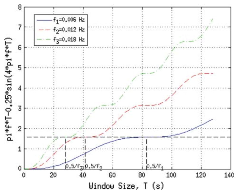
Simulation result of three sinusoidal signals, with frequencies f₁ = 0.006Hz, f₂ = 0.012 Hz and f₃ = 0.018Hz. The function plotted is a measure of expected value of the time-windowed correlation between two sinusoids with same frequency, but with two different realizations of zero-mean unit-variance white noise superimposed. 0.5/f_i, i = 1, 2, 3, correspond to window size that has the first (non-zero) saddle-point of the function. The saddle-point guides the “optimal” window size selection in dynamic correlation analysis

Three results can be observed from the plot and can be theoretically verified:

• (R1) the function has a first (non-zero) saddle-point at T = 0.5/f,

• (R2) value of the function at the first saddle-point is π/2 and it is independent of frequency, f,

• (R3) the higher the frequency, f, the greater the function’s value,

• (R4) the higher the frequency, f, the smaller the window size, T, that corresponds to the first (non-zero) saddle point.

Given that one should select a small window size for dynamic analysis, it is reasonable to select a window size which is close to the saddle point of the lowest frequency component present in the BOLD signal. For example, for the sinusoid with f = 0.006Hz, selection of 95% of the saddle-point value, π/2, would correspond to a window size of approximately T = 64 s. As expected, the lowest interesting frequency component present in our signal sets the upper limit on window size and is usually determined by the lower cutoff of the temporal filter applied to the signal during preprocessing in fMRI. Similarly, the highest interesting frequency component, which represents the fastest changes of interest in signal, determines the lower limit on the window size. One can then set a percentage value (e.g. 95%) and that would dictate the window size in a dynamic correlation analysis. One can select window sizes greater than this value, but this value sets a guidance maximum value. Selection of window size that corresponds to the lower limit of frequency content of signal seems to be optimal; however, one can choose to be more conservative. If the chosen window size is too long, fast changes can no longer be modeled. For example, a conservative selection could be 150% of this value, but 200% seems to be too long, based on our simulations (not shown here).

Simulation

Based on the theoretical assessment in the previous section, we selected three zero-mean unit variance sinusoid signals that correspond to frequencies f₁ = 0.006Hz, f₂ = 0.012 Hz and f₃ = 0.018Hz and we constructed a fourth signal that was a temporally piece-wise combination of these three. Then, zero-mean Gaussian random noise with 0.25 standard deviation was added to the signals. Cross-correlation values between signal pairs were calculated (static correlation). 28 different random noisy realizations of this was generated (corresponding to number of subjects per group, 28, in our fMRI study) and the results averaged. For dynamic connection analysis simulations, signals were windowed with a sliding-window size of 64s. As a result, for each signal pair, dynamic correlation values (per every sliding-window), averaged over 28 realizations, were obtained. The simulation results are presented in Fig. 1. Simulation results based on sinusodial signals with different frequencies are presented in Fig. 2. In Fig. 1, it can be observed that the window number 0.5/f_i, i = 1, 2, 3, corresponds to window size that has the first (non-zero) saddle-point of the function.

Fig. 2.

Simulation results showing the difference between dynamic and static connectivity analysis. a Zero-mean unit standard deviation periodic signals used for simulation. The last signal is a piece-wise combination of the first three. b Dynamic cross-correlation values among the signal pairs, averaged over 28 repetitions, when Gaussian random noise with 0.25 std is added and repeated (window size=64s). It also includes average static correlation values (labeled ‘static cc’)

The saddle-points, therefore, provide guidance for setting the “optimal” window size in dynamic correlation analysis. Four sinusoidal signals, with different frequencies, are presented in Fig. 2a. The first three signals have three distinct frequencies and therefore they are expected to have low cross-correlation. However, signal 4 is constructed by combining the three sinusoids in a time-multiplexed manner (i.e. the first 1/3rd of the period is equal to the first signal, the middle 1/3rd of the period is equal to the second signal and so on), and therefore signal 4 is expected to have some degree of correlation with the other signals at different times. Static and dynamic correlation results among the 6 pairs, with window size of 64 s, are presented in Fig. 2b. Cross correlation values between these noisy signal pairs, repeated and averaged over 28 realizations, are calculated and presented (static correlation coefficient (cc), labeled ‘static cc’ in each of the 6 plots). Signal pairs 1–4, 2–4 and 3–4 all have significant static correlation of ~0.33(P = 3 × 10⁻¹², n = 498), while the rest of the pairs have correlations near zero. Thus, although signal 1 and signal 4 are related only for 1/3rd of the total signal duration, the use of static correlation values between them would lead to the conclusion that the two signals are correlated, which would imply functional connection.

The dynamic correlation plots provide a more detailed story on connectivity. For dynamic connection analysis simulations, signals were windowed with a sliding-window size of 64. As a result, for each signal pair, dynamic correlation values (per every sliding-window), averaged over 28 noisy realizations, were obtained. As can be seen in the dynamic cc plot for pair 1–4 in Fig. 2b, the dynamic correlation values are quite high (between 0.76 and 0.96) for the first 1/3rd of the windows (between 48 and 272 s) and lower for the rest of the windows with occasional high peaks. Similar conclusions can be drawn for pair 2–4 and pair 3–4; the distinction of time period where the pair is correlated gets better for pair 2–4 and is the best for pair 3–4, since the frequency content increases and it is easier to single out the time period where there is very good connectivity (middle 1/3rd of the windows for pair 2–4 and last 1/3rd of the windows for pair 3–4). Overall, the simulations show us that the dynamic correlation analysis provides us with a measure of the temporal evolution of the correlation value, hence the temporal evolution of functional connectivity.

Application to fMRI data

Participants

Participants consisted of 28 right-handed chronic schizophrenia patients (SP) and 28 healthy controls (HC). SP were outpatients referred by Hartford Hospital physicians. HC were recruited from the local community through newspaper advertisements, pamphlets, and postings. All of the participants gave written, informed consent to the study, which was approved by the Internal Review Board of Harford Hospital. Any participants with mental retardation (full scale IQ < 70), visual and auditory impairment, or traumatic brain injury with loss of consciousness greater than 15min, were excluded from the study. HC participants with any medical, neurological, or psychiatric illnesses such as DSM-IV TR Axis I disorder or psychiatric/psychotropic medication were excluded. Participants with history of substance abuse or substance dependence in the past 6 months were also excluded. Candidates were screened by a urine toxicology test on the day of scanning and those with positive results excluded. Prior to scan, all participants were asked to practice the oddball task; those who could not were also excluded. Schizophrenia was diagnosed using DSM-IV TR criteria on the basis of a clinical SCID interview [50] and review of medical file. Mean ± standard deviation (SD) age at the time the scan was 28.8 ± 10.7 for HC (19 males, 9 females) and 36.4 ± 12.4 for SP (23 males, 5 females).

Experimental design and task

All participants were scanned during both an auditory odd-ball task and while resting, eyes open visually fixating on a cross. The auditory oddball task (AOT) consisted of detecting an infrequent sound within a series of regular and different sounds [30,51]. The task consisted of two runs of auditory stimulus presented to each participant by a computer stimulus presentation system (VAPP) via insert earphones embedded within 30-dB sound attenuating MR compatible headphones. The standard stimulus was a 500-Hz tone, the target stimulus was a 1,000-Hz tone, and the novel stimuli consisted of non-repeating random digital noises (e.g., tone sweeps, whistles). The target and novel stimuli each occurred with a probability of 0.10 and the standard stimuli occurred with a probability of 0.80. The stimulus duration was 200ms with a 1,000, 1,500, or 2,000ms interstimulus interval. All stimuli were presented at 80-dB above the standard threshold of hearing. All participants reported that they could hear the stimuli and discriminate them from the background scanner noise. Prior to entry into the scanning room, each participant performed a practice block of 10 trials to ensure understanding of the instructions. The participants were instructed to respond as quickly and accurately as possible with their right index finger every time they heard the target stimulus and not to respond to the nontarget stimuli or the novel stimuli. An MRI compatible fiber-optic response device (Lightwave Medical, Vancouver, BC) was used to acquire behavioral responses for both tasks. A detailed description of the AOT stimulus paradigm, the data acquisition techniques and previously found stimulus-related activation can be found in relevant work by Kiehl et al. [30,51,52]. A sample auditory oddball task paradigm is presented in Fig. 3. Two runs of the experiment were performed, and each run lasted 6.5 min.

Fig. 3.

Sample auditory oddball task paradigm. The stimulus consisted of three different kinds of tones: standard (0.5kHz tone), target (1kHz tone) and novel (random tones of sweep & whistle). Stimulus duration was 200ms with interstimulus interval of 500, 1,000 or 1,500ms

Participants also performed a 5-min resting state scan (REST) for complete data-collection. Participants were instructed to rest quietly without falling asleep with their eyes open (eyes were open to avoid the possibility that participants would fall asleep). The results based on the resting-state data analysis are not included in this paper and they are the subject of a separate study.

Imaging system and parameters

A Siemens Allegra 3T MR system (Siemens, Erlangen, Germany) equipped with 40 mT/m gradients and a standard quadrature head coil was used for data collection. Scans were acquired at the Olin Neuropsychiatry Research Center at the Institute of Living/Hartford Hospital. Functional scan parameters were as follows: Gradient-echo echo-planar-imaging in the transaxial plane, repetition time (TR)=1.50s, echo time (TE)=27ms, flip angle=70°, field of view=24cm, acquisition matrix=64×64, voxel size=3.75×3.75×4 mm³, slice thickness/gap=4 mm/1 mm, number of slices=29, ascending acquisition. The scan started automatically by a trigger from the task paradigm controller. The task fMRI data had 249 volumes in each run after discarding the 6 initial scans for longitudinal equilibrium. There were two back-to-back, separate runs for the task, and the data from the two runs were concatenated, resulting in 498 volumes.

Data preprocessing

The standard preprocessing steps (realignment/motion-correction and normalization) were performed via the MATLAB-based (http://www.mathworks.com) SPM5 package (http://www.fil.ion.ucl.ac.uk/spm/software/spm5). For motion correction, the INRIalign algorithm was used [53]. Motion corrected data were spatially normalized to Montréal Neurological Institute (MNI) standard-space (results in data being resampled to 3 × 3 × 3 mm³, with matrix size 53 × 63 × 46). Data were then smoothed by a 3D Gaussian kernel with full-width at half-maximum of 10×10×10 mm³ and converted into 2-D matrix of time-by-voxels.

Group spatial ICA

Group ICA of fMRI Toolbox (GIFT, http://icatb.sourceforge.net) was used to compute spatially independent components (ICs) [23]. Group sICA steps are summarized in Fig. 4.

Fig. 4.

Summary of preprocessing and group spatial ICA steps. After each subject’s fMRI data are motion-corrected and spatially normalized to a common template, thus their voxels are aligned. The normalized data are flattened to a T-by-V matrix, where T is number of time-points and V is number of voxels. After normalization, H number of subjects for group 1 and P number of subjects for group 2 are temporally concatenated and the resulting (H + P)T -by-V matrix X is fed into group sICA algorithm. Group sICA finds C number of maximally independent (spatially) components. Each component’s spatial extent is described by C rows of the matrix S as a result of sICA. Each component has an associated time-course, for each subject (C columns of matrix A). X = AS

Principal component analysis (PCA)-based compression was used in the temporal domain before the ICA on the subject data and also on the temporally concatenated group data. The number of ICs in group ICA was estimated to be C = 19 by using the modified minimum description length criteria [54]. Group ICA was then performed using the Infomax algorithm [22]. After spatial reconstruction and visual inspection of the 19 components, C′ = 10 components-of-interest were selected for the FNC study.

Static and dynamic FNC analysis

Static FNC analyses were performed using the FNC Toolbox developed by Calhoun et al. (http://mialab.mrn.org/software) based on the maximal lagged correlation approach [6]. For each subject, the 10 time-series associated with the selected ICs/networks were band-pass filtered between 0.013 and 0.133Hz, upsampled (12×) for accurate lag estimation, and normalized to zero-mean unit-variance. These time-series for each subject were then paired to obtain (C′, 2) = 45 combinations. The lag estimation and maximal lagged correlation values were then computed by using the maximal lag correlation approach [6]. The correlation values obtained by using the whole time-courses were noted as a measure of static functional connectivity between the networks. Then, the group difference for these connections was tested by using t-test with a P-value threshold of 0.01. A summary of the steps involved in static FNC is provided in Fig. 5.

Fig. 5.

Summary of steps involved in static FNC. Out of C components, a subset C′ components of interest are selected. Each of these components’ associated time-courses are then paired and maximal lagged correlation is calculated, resulting in C′-by-C′ static connectivity matrix for each subject. Then group statistics of the connectivity matrix, such as mean and standard deviation, are computed and significance and group difference significance of the connectivity matrix is tested based on these group statistics

For the dynamic FNC analysis, the lags were first accounted for by offsetting for the existing lags between each time-course pair. Each time-course had 498 samples (time-points), which corresponds to a duration of 747s (recall that TR = 1.5s). Using time-windows of length 96s (i.e. 64 time-points) with window step size of 3s (i.e. 2 time-points) resulted in W = 498/2 − 64/2 + 1 = 218 windows. Window step size is the duration of the temporal shift between each window as the windows are shifted forward in time at each step. The window size was conservatively chosen to correspond to 0.75/f, 150% of the minimal limit set by the simulation, where f = 0.013Hz corresponds to the lowest frequency component of the time-courses. For each time-window, the correlation values were calculated for each subject, for each pair. For computational purposes, pre-offsetting for lags was calculated once for the time-course pair, rather than calculating it for all 218 time-windowed time-course pairs. The pre-offsetting allowed a more stable calculation of lags since the whole time-course was used. It also decreased the computation time to within reasonable levels (~218times less computation time). As a result, for each of the n₁ + n₂ = 56 subjects and for each of the 45 time-course pairs, 218 correlation values were obtained, which provided a measure of dynamics of functional connectivity of the selected networks. For each group, the mean and standard deviation of these 218 correlation values were computed (n₁ = n₂ = number of subjects = 28). Two-sampled t-test for group difference in correlation values for each of the 218 windows was applied and significance of the group difference was assessed by studying the resulting P-values. Since the resulting P-values also change over time for each of the windows, this provided an assessment of the dynamics of significance of the group difference in connectivity over the course of the experiment. A summary of the steps involved in dynamic FNC steps is provided in Fig. 6.

Fig. 6.

Summary of steps involved in dynamic FNC. Out of C components, a subset C′ components of interest are selected (same components selected in static FNC analysis). Each of these components’ associated time-courses are time-windowed, resulting in W versions, where W is number of sliding and overlapping time-windows. For each time-window, the time-courses are paired and maximal lagged correlation is calculated, resulting in W number of (dynamic) C′-by-C′ connectivity matrices for each subject. Then group statistics of connectivity matrices, such as mean and standard deviation, are computed and significance and group difference significance of the connectivity matrices are tested based on the group statistics

Task modulation of dynamic FNC

In addition to studying dynamic correlation, relationship of dynamic correlation values with the task, i.e., the measure of task-modulation, was also studied. First, a ‘task-load function’ was generated by computing the time-windowed integral of the HRF-convolved event-related task paradigm. The task-load function provides a measure of how much the subject was engaged with the task within the computation window. By correlating the dynamic correlation values with the task-load function, the relationship between the evolution of connectivity with the task was studied, which basically tries to answer the question “is the connection between the network pair being modulated by the task?”

Whether the task-modulation (of connectivity) differed significantly for the two groups, for each of the network pairs, was also investigated. To do this, R² value of the fitting of the task-load function to the dynamic correlation coefficients between all IC pairs, was calculated. A summary of task-modulation of dynamic FNC analysis steps is presented in Fig. 7.

Fig. 7.

Summary of task-modulation analysis with dynamic FNC. For each subject, a particular element {i,j}s of dynamic C′-by-C′ connectivity matrix has W values which corresponds to dynamic correlation coefficient (cc) of the component pair i–j. The dynamic cc for every component pair is correlated with the task-load function and the result is C′-by-C′ matrix of ‘task-modulation’ for each subject. Group statistics (mean and standard deviation) are calculated and significantly task-modulated pairs, or FNCs, in each group and pairs with significant group difference in task-modulation are calculated based on these statistics. The task-load function is obtained by convolving the task onsets with a hemodynamic response function, and then by averaging using the sliding window

The dynamic FNC analysis was basically a repeat of the static FNC analysis, except that the inputs to dynamic FNC were time-windowed, short, component time-courses representing many different periods during the experiment, rather than whole component time-courses that encompassed the whole period of the experiment. Dynamic FNC results were used to assess task-modulation by measuring their correlations with the task-load function obtained from the empirical hemodynamic response function. An overall summary of static and dynamic FNC analysis steps is presented in Fig. 8.

Fig. 8.

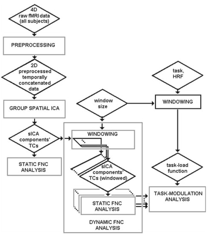
Summary of overall analysis steps. Dynamic FNC analysis is basically a repeated version of static FNC analysis except that the input to dynamic FNC are time-windowed, short, component time-courses that belong to many different periods during the experiment rather than whole component time-courses that belong to whole period of the experiment. Dynamic FNC results can then be used to assess task-modulation, by using the task-load function. The task-load function is obtained by convolving the task onsets with a hemodynamic response function, and then by averaging using the same sliding window

Bootstrapping

Bootstrapping was applied to the network pairs that showed significant group difference (P < 0.05) in order to investigate the robustness of results. Twenty subjects from each group were randomly selected and the task-modulation of dynamic FNC was applied by using these SP and HC subgroups. The P-value of group difference in task-modulation was calculated. This was repeated 1,000 times, each time by selecting 20 subjects randomly in each group. For each pair, percentage of the time for which P < 0.05, or the frequency of occurrence of significant difference, was calculated. Bootstrapping was also applied to the static FNC analysis and the percentage of occurrence for the significance in connections was calculated (again, 20 random subjects per subgroup, 1,000 random repetitions).

Time–frequency analysis of dynamic FNC

The dynamic time–frequency representation (TFR) of the connectivity difference between groups was also studied. For all subjects, the IC time-courses were paired and then the difference signal for the pair was obtained by subtracting one time-course from another (after the standard preprocessing of normalizing them to zero mean and unit variance and after shifting by the amount of the time lag that provides the maximal cross-correlation for a pair). The same window in dynamic FNC analysis was applied to the difference signal, and the Fast Fourier Transform (FFT) of the windowed difference signal was computed. An FFT for each window was obtained for each window. The result is a time–frequency surface for the pair’s difference signal showing the dynamic evolution of the frequency content of the difference, which is called the TFR. TFRs of the subjects within each group were averaged for both groups, and the TFR difference of the two groups was obtained by subtracting the SP group’s average TFR from the HC group’s average. This was performed for all IC pairs. The areas in the TFR difference which are significant were calculated by t-test and were delineated by contours. The results for the pairs of interest are presented. The frequency scale of the plots are clipped between 0.01 and 0.1Hz. The results are interpreted and they are compared with those of the dynamic FNC analysis.

Results

Ten selected ICA components are presented in Fig. 9, are as follows: (a) IC#1: motor network (M), (b) IC#2: right lateral fronto-parietal network (RLFP), (c) IC#5: medial visual network (mV), (d) IC#7: orbito-frontal network (OF), (e) IC#8: posterior default mode network (pDM), (f) IC#9: parietal network (P), (g) IC#12: anterior temporal network (aT), (h) IC#16: medial temporal network (mT), (i) IC#18: frontal network (F), and (j) IC#19: left lateral fronto-parietal network (LLFP).

Fig. 9.

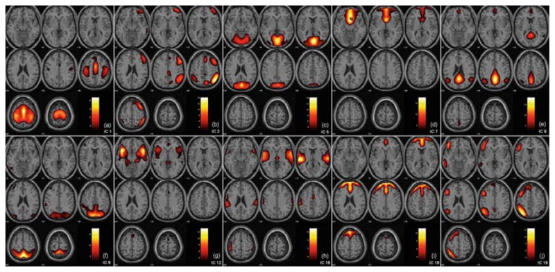
Ten selected spatial ICA components (networks). a IC#1: motor network (M), b IC#2: right lateral fronto-parietal network (RLFP), c IC#5: medial visual network (mV), d IC#7: orbito-frontal network (OF), e IC#8: posterior default mode network (pDM), f IC#9: parietal network (P), g IC#12: anterior temporal network (aT), h IC#16: medial temporal network (mT), i IC#18: frontal network (F), and j IC#19: left lateral fronto-parietal network (LLFP)

HC–SP static FNC group difference results are presented in Fig. 10. The HC group has significantly greater (P < 0.01) 1mV–F connection, mT–mV connection, P–mT connection, P–mV connection and mT – aT connection. Only the RLFP–OF connection was significantly greater in SP (P < 0.01, arrow not shown). These differences were also validated by applying bootstrapping; 20 subjects per group were randomly selected, static FNC analysis was done and this was repeated for 1,000 times. The percentages of the occurrences for which there was a significant group difference (P < 0.01) were calculated and they are all practically 100% for all the pairs.

Fig. 10.

HC–SP static FNC analysis results. Connections with significant group difference are shown (P < 0.01). The lag differences are ignored (lag difference P < 1). Bootstrap results with 20 subjects per group, 1,000 randomized trials, resulted in 100% occurrence (of the significant group difference of the same connections)

After the dynamic correlation coefficients were computed for each IC pair, the group average was calculated for all the pairs. Correlation of dynamic correlation coefficient values with the task-load function (i.e. the R² values of the fitting), averaged for each group, are presented in Table 1 (for 8 pairs that show significance in group difference). Temporal evolution of group-averaged correlation coefficients between selected IC pairs for patients (green) and controls (blue) is shown in Fig. 11a. The task-load function (in red) is also presented for reference. The first five of these pairs in this figure (M–F pair, RLFP–mT pair, OF–pDM pair, pDM–P pair and mT–F pair) were selected based on the criteria of whether they showed a significant group difference in task-modulation. For these pairs, the P-values of group differences for 2-sample t-test were all less than 0.025. As can be seen from Table 1, RLFP network–medial temporal network connectivity and medial temporal network–frontal network connectivity exhibited a significantly higher task modulation in the HC group than in the SP group. Motor network–frontal network connectivity, orbitofrontal network–posterior default mode network connectivity and posterior default mode network–parietal network connectivity exhibited a significantly higher task-modulation in the SP group. Two other pairs, the mV–LLFP pair and OF–mT pair, also showed nearly significant (P < 0.067) group difference in task-modulation and their connectivities were higher in the HC group. The last pair of interest, the RLFP–LLFP pair, was selected to study lateral connectivity by using the symmetrically lateral left and right LFP networks that appeared as ICs. There was not any significant HC versus SP group difference (P = 0.48) in the RLFP–LLFP connectivity in terms of task-modulation.

Table 1.

Statistical results of task-modulation of connectivity

IC Pair	Avg. 〈 cc, task 〉		HC–SP (T-test)	Bootstrap results (N1=N2=20, Repetition=1,000)
	HC	SP	P-value	P < 0.05 (%)
IC#1 (M) &IC#18 (F)	0.0604	0.1221	0.0107 (SP>HC)*	69.4
IC#2 (RLFP) &IC#16 (mT)	0.1069	0.0562	0.0223 (HC>SP)*	54.6
IC#2 (RLFP) &IC#19 (LLFP)	0.0974	0.0960	0.4815 (HC>SP)
IC#5 (mV) &IC#19 (LLFP)	0.1173	0.0786	0.0655 (HC>SP)
IC#7 (OF) &IC#8 (pDM)	0.0528	0.0951	0.0128 (SP>HC)*	63.5
IC#7 (OF) &IC#16 (mT)	0.0868	0.0564	0.0566 (HC>SP)
IC#8 (pDM) &IC#9 (P)	0.0456	0.0970	0.0133 (SP>HC)*	69.1
IC#16 (mT) &IC#18 (F)	0.0708	0.0376	0.0195 (HC>SP)*	55.0

R² value of regression of dynamic average correlation coefficients with the task load function for all component pairs, for the two groups and P value of the group difference. The component pairs marked with ‘*’ show significant group difference, hence show significant group difference (P < 0.05) in specified task modulation of the functional connectivity between the specified component pair. None of them are significant when the Bonferroni correction is applied (P < 0.002). When a false discovery rate of P < 0.05 was applied, the cut-off value in the original P values was 0.0223. Bootstrapping results, in terms of percentage of the subgroups that provide P < 0.05 are also provided. Subgroups consisted of 20 subjects randomly chosen out of 28 subjects per each group and 1,000 random repetitions

^*Statistically significant (P < 0.05)

Fig. 11.

Dynamic FNC analysis results. a Temporal evolution of average correlation coefficient for the two groups (blue: HC group average, green: SP group average), for selected pairs. Temporal evolution of task-load (red) is also presented for comparison. b Corresponding dynamic P-values of group significance of the dynamic correlation for these pairs

The pairs of networks that exhibited significant group difference in Table 1 also exhibited significance of group difference when the false discovery rate correction with P < 0.05 was applied. This rate corresponded to a cutoff rate of P < 0.0223 in the original P-values. None of these pairs exhibited significance of group difference when the Bonferroni correction was applied (P < 0.002). Bootstrapping results for these pairs of networks reveal that the group differences (P < 0.05) in task modulation of their connections were confirmed 55–70% of the time when different subgroups were selected (20 random subjects per subgroup, 1,000 repetitions). It is interesting to note that the pairs for which the SP group had more task-modulation (M–F, OF–pDM, pDM–P connections) had higher percentages of confirmation (70, 64, 70%, respectively) than the pairs for which the HC had more task-modulation (RLFP–mT, mT–F, both 55%).

The plots in Fig. 11b present the corresponding dynamic P-values of significance tests in HC–SP group difference in connectivity (which should not be confused with the group difference in task-modulation of connectivity), for the same eight selected pairs of interest. From these plots, it can be seen that the P-values (and hence does the group difference) fluctuate. One observation that can be made from this figure is that the OF–pDM connectivity provides the highest level group difference as the P-values of group difference for this connectivity, except the first quarter of the experiment, are the lowest and P < 0.05 for more than 50% of the time (windows).

The HC–SP group difference in average time–frequency representation of the dynamic correlation coefficients for the selected pairs are presented in Fig. 12.

Fig. 12.

Group difference of HC–SP time–frequency plot of the average group correlations for the selected component pairs

The x-axis of the plots in Fig. 12 represents the window number, while the y-axis represents the frequency (between frequencies 0 and 0.1Hz). The red contours delineate the time–frequency surfaces where the HC group’s time–frequency representation of connectivity are significantly greater than those of the SP group (P < 0.05), and the blue contours represent the time–frequency areas where the opposite is true. It can be observed that, for these pairs, the sizes of red-contoured areas are significantly greater than the sizes of the blue-contoured areas (about 37 times more, on average, P < 0.01), i.e., the HC group had larger time–frequency areas that are significantly higher (P < 0.01) for the pairs of interest. This means that the HC group has more overall connectivity within the 0–0.1Hz frequency band, among these pairs of interest. However, for orbito-frontal and posterior default mode connectivity, the sizes of red-contoured areas are only slightly significantly greater than the sizes of the blue-contoured areas (only 1.8 times more, P < 0.05), and both areas are smaller when compared with the rest of the selected pairs.

Discussion

The static and dynamic FNC analyses each revealed answers to different but complementary questions about group differences in brain activity. Static FNC analysis revealed “which connections show significant group differences?” and dynamic FNC analysis revealed “which connections’ task-modulations show significant group difference?” The static FNC results revealed that connectivities involving mV–F, mT–mV, P–mT, P–mV and mT–aT were higher in HC whereas only the RLFP–OF connection was significantly greater in SP. The dynamic FNC revealed that other sets of connections, M–F, RLFP–mT, OF–pDM, pDM–P, and mT–F, showed significant group differences in task modulation. It is interesting that no connections involving the default mode, pDM, showed significant group difference in static connectivity. However, the pDM’s connectivity with two networks (OF and P) showed significant task modulation difference between the two groups. The dynamic FNC revealed DM-related group differences by enabling assessment of task-modulation.

The default mode, which should be expected to be anti-correlated with task-related networks and the network least functionally connected to the rest of the brain networks during an explicit task, exhibited more connectivity, or more similar temporal behavior, to the orbito-frontal network in HC during the auditory oddball task. Dynamic FNC analysis revealed that this difference was not significant (average dynamic P-value ~ 0.07). This was also the case using static FNC analysis (group difference of static connectivity, P > 0.05, with connectivity in HC being greater). This suggests that the default mode is functionally less segregated than the rest of the networks which are involved in motor and cognitive functions in schizophrenia patients, when the subject is engaged with task that involves motor and cognitive functions. However, it should be noted that the difference is not significant. This difference could be due to motor and/or cognitive deficits in schizophrenia.

The medial temporal network, which is expected to be highly active during auditory tasks, showed more connectivity to other functional networks, including parietal and right lateral fronto-parietal networks in the HC group during the task. This means that these networks might be ‘communicating’, ‘functionally connecting’ or ‘integrating’ better in healthy controls while performing the task. It seems consistent that the degree of communication between these regions which are responsible for cognitive and audiosensory functions, is greater in healthy controls, consistent with hypotheses that schizophrenia disrupts cognitive and sensory functions [33,34,42,43].

The dynamic connectivity of orbitofrontal–posterior default mode networks shows a large group difference for most of the experiment duration. This pair also exhibited a significant group difference in task-modulation of its dynamic connectivity. Provided that this is evaluated in greater subject populations, the dynamic connectivity of orbitofrontal–posterior default mode can potentially be used as a feature in diagnostic classification algorithms for schizophrenia. In general, classification of groups based on dynamic functional connectivity analysis of certain networks is the subject of further future research and is part of our ongoing research [49].

The bootstrap results revealed that the dynamic FNC results, i.e., the group differences in task-modulation of selected networks, were verifiable in most of the subgroups, but not robust. The static FNC results were robust when bootstrapping was applied. The robustness in static FNC is because more temporal data points are used in its calculation when compared with the dynamic FNC.

It was observed in time–frequency analysis for the component pairs of interest that the HC group had significantly more overall connectivity within the 0–0.1Hz frequency band. Interestingly, this result was less pronounced for orbito-frontal and posterior default mode connectivity. This means that time–frequency representation of the connectivity of this pair does not seem to be very significantly different for the SP and HC groups. While this might not be expected, given that we observed a group difference in orbito-frontal and posterior default mode connectivity (Fig. 11b) and significant difference in task-modulation of its connectivity (Fig. 11a), the high variance of the time–frequency representation within the groups for this pair contributes to this result.

Based on simulation and application results, it is clear that the dynamic FNC approach provides more insights than the static FNC analysis. Dynamic FNC enables an assessment of the task-modulation of the connections between networks. The hypothesis that “functional connectivity among the different brain networks is dynamic” can be assessed and tested by dynamic analysis, as done in this work. The static FNC provides us with overall connectivity during the course of experiment. If functional connectivity is assumed and modeled as static during the course of fMRI experiments, that is, if the dynamics of the connections are not modeled and assessed, mistaken conclusions can be drawn from studies that have different underlying dynamics but the same average effect over time [55].

The simulations performed in this work showed that the lowest frequency content of the signal dictates the minimum window size. If one sets a window size smaller than the period of the lowest valuable frequency component of the signal, then the effect of that component is lost. In our work we used more than the required minimum window size. For different data sets, there might be different factors forcing the window size, depending on the sample size, data quality, filtering, etc. If the frequency content of the signal changes during the course of the experiment, and if it can be detected by an adaptive algorithm, an adaptive scheme could also be developed to adjust the window size accordingly. This would be important in scenarios where the dynamic FNC analysis is in real- or near-real time.

Although the FNC analysis was performed in a dynamic fashion, the sICA components, or networks, were spatially fixed and they were estimated from the whole fMRI data set. As we noted previously, the sICA components can be estimated dynamically [26] by using windowed fMRI data, and the dynamic FNC analysis can be done concurrently just after the dynamic sICA estimation at every window step. Also, the networks, and the functional connectivity of these networks can be estimated and updated in an incremental manner (as in Kalman Filtering), where previously estimated networks based on previous window steps could be provided as an input, or prior, to the ICA and FNC algorithms in the subsequent windows steps. If the computational complexity of this scheme can be overcome, this fully dynamic scheme would enable real-time or near real-time dynamic incremental FNC analysis based on real-time dynamic incremental ICA.

In this work, correlation coefficients were used as a measure of connectivity. We did not perform a Fisher Transform before testing for statistical significance, however the time-courses were normalized to have (approximately) same standard deviation. Almost all of the correlation values in our study were less than 0.5, and for correlation values less than 0.5 the Fisher transform has little effect on the significance of the results.

The dynamic FNC analysis method introduced in this work and other previous works which study the dynamics of FNC suggest that the functional network connectivity of the brain is likely dynamic (i.e., involves temporally changing characteristics). The advantages of the method developed here, when compared to other methods such as Bayesian methods [21], dynamic causal modeling (DCM) [20,56] or structural equation modeling (SEM) [18] is that these methods are model-based and they are limited by the complexity and the underlying assumptions of their models. These models all assume that certain interaction parameters describe the relation among voxels or segregated, clustered, functional networks, and they try to estimate these parameters. The ICA-based dynamic FNC method does not have any underlying assumptions other then Gaussianity and linear mixing as explained in the introduction section of this paper.

Conclusions

We performed a dynamic functional network connectivity analysis of spatially independent networks in healthy controls and schizophrenia patients during an auditory oddball task and compared the two groups. Based on spatial ICA and dynamic (time-windowed) FNC analysis, we developed a method for assessing task-modulation of functional network connectivity. The task-modulation of dynamic FNC provided findings and group differences in the two groups that are consistent with the existing hypothesis that schizophrenia patients show fewer segregated motor, sensory, cognitive functions and less default mode network activity when engaged with a task. These findings corroborate and extend the previous findings related to the abnormalities seen in schizophrenia in sensory, motor and cognitive functions and their integration. Future work involves fully dynamic and concurrent estimation of networks and their functional connectivity.

Abbreviations

fMRI

Functional magnetic resonance imaging

FC

Functional connectivity

FNC

Functional network connectivity

DFNC

Dynamic functional network connectivity

ICA

Independent component analysis

sICA

Spatial independent component analysis

SP

Schizophrenia patients

HC

Healthy controls

AOT

Auditory oddball task

References

- 1.Biswal B, Yetkin FZ, Haughton VM, et al. Functional connectivity in the motor cortex of resting human brain using echoplanar MRI. Magn Reson Med. 1995;34:537–541. doi: 10.1002/mrm.1910340409. [DOI] [PubMed] [Google Scholar]
- 2.Biswal BB, Van Kylen J, Hyde JS. Simultaneous assessment of flow and BOLD signals in resting-state functional connectivity maps. NMR Biomed. 1997;10:165–170. doi: 10.1002/(sici)1099-1492(199706/08)10:4/5<165::aid-nbm454>3.0.co;2-7. [DOI] [PubMed] [Google Scholar]
- 3.Lowe MJ, Mock BJ, Sorenson JA. Functional connectivity in single and multislice echoplanar imaging using resting-state fluctuations. Neuroimage. 1998;7:119–132. doi: 10.1006/nimg.1997.0315. [DOI] [PubMed] [Google Scholar]
- 4.Cordes D, Haughton VM, Arfanakis K, et al. Mapping functionally related regions of brain with functional connectivity MR imaging. AJNR Am J Neuroradiol. 2000;21:1636–1644. [PMC free article] [PubMed] [Google Scholar]
- 5.Cordes D, Haughton V, Carew JD, et al. Hierarchical clustering to measure connectivity in fMRI resting-state data. Magn Reson Imaging. 2002;20:305–317. doi: 10.1016/s0730-725x(02)00503-9. [DOI] [PubMed] [Google Scholar]
- 6.Jafri MJ, Pearlson GD, Stevens M, et al. A method for functional network connectivity among spatially independent resting-state components in schizophrenia. Neuroimage. 2008;39:1666–1681. doi: 10.1016/j.neuroimage.2007.11.001. [DOI] [PMC free article] [PubMed] [Google Scholar]
- 7.Assaf M, Jagannathan K, Calhoun V, et al. Temporal sequence of hemispheric network activation during semantic processing: a functional network connectivity analysis. Brain Cogn. 2009;70:238–246. doi: 10.1016/j.bandc.2009.02.007. [DOI] [PMC free article] [PubMed] [Google Scholar]
- 8.Calhoun VD, Kiehl KA, Pearlson GD. Modulation of temporally coherent brain networks estimated using ICA at rest and during cognitive tasks. Hum Brain Mapp. 2008;29:828–838. doi: 10.1002/hbm.20581. [DOI] [PMC free article] [PubMed] [Google Scholar]
- 9.Maldjian JA, Laurienti PJ, Kraft RA, et al. An automated method for neuroanatomic and cytoarchitectonic atlas-based interrogation of fMRI data sets. Neuroimage. 2003;19:1233–1239. doi: 10.1016/s1053-8119(03)00169-1. [DOI] [PubMed] [Google Scholar]
- 10.Baumgartner R, Windischberger C, Moser E. Quantification in functional magnetic resonance imaging: fuzzy clustering vs. correlation analysis. Magn Reson Imaging. 1998;16:115–125. doi: 10.1016/s0730-725x(97)00277-4. [DOI] [PubMed] [Google Scholar]
- 11.Baumgartner R, Scarth G, Teichtmeister C, et al. Fuzzy clustering of gradient-echo functional MRI in the human visual cortex. Part I: reproducibility. J Magn Reson Imaging. 1997;7:1094–1101. doi: 10.1002/jmri.1880070623. [DOI] [PubMed] [Google Scholar]
- 12.Lu N, Shan BC, Xu JY, et al. An improved temporal clustering analysis method applied to whole-brain data in fMRI study. Magn Reson Imaging. 2007;25:57–62. doi: 10.1016/j.mri.2006.09.034. [DOI] [PubMed] [Google Scholar]
- 13.Meyer FG, Chinrungrueng J. Spatiotemporal clustering of fMRI time series in the spectral domain. Med Image Anal. 2005;9:51–68. doi: 10.1016/j.media.2004.07.002. [DOI] [PubMed] [Google Scholar]
- 14.Backfrieder W, Baumgartner R, Samal M, et al. Quantification of intensity variations in functional MR images using rotated principal components. Phys Med Biol. 1996;41:1425–1438. doi: 10.1088/0031-9155/41/8/011. [DOI] [PubMed] [Google Scholar]
- 15.Friman O, Cedefamn J, Lundberg P, et al. Detection of neural activity in functional MRI using canonical correlation analysis. Magn Reson Med. 2001;45:323–330. doi: 10.1002/1522-2594(200102)45:2<323::aid-mrm1041>3.0.co;2-#. [DOI] [PubMed] [Google Scholar]
- 16.McKeown MJ, Makeig S, Brown GG, et al. Analysis of fMRI data by blind separation into independent spatial components. Hum Brain Mapp. 1998;6:160–188. doi: 10.1002/(SICI)1097-0193(1998)6:3<160::AID-HBM5>3.0.CO;2-1. [DOI] [PMC free article] [PubMed] [Google Scholar]
- 17.Neufang S, Fink GR, Herpertz-Dahlmann B, et al. Developmental changes in neural activation and psychophysiological interaction patterns of brain regions associated with interference control and time perception. Neuroimage. 2008;43:399–409. doi: 10.1016/j.neuroimage.2008.07.039. [DOI] [PubMed] [Google Scholar]
- 18.Buchel C, Friston KJ. Modulation of connectivity in visual pathways by attention: cortical interactions evaluated with structural equation modelling and fMRI. Cereb Cortex. 1997;7:768–778. doi: 10.1093/cercor/7.8.768. [DOI] [PubMed] [Google Scholar]
- 19.Astolfi L, de Vico Fallani F, Cincotti F, et al. Imaging functional brain connectivity patterns from high-resolution EEG and fMRI via graph theory. Psychophysiology. 2007;44:880–893. doi: 10.1111/j.1469-8986.2007.00556.x. [DOI] [PubMed] [Google Scholar]
- 20.Friston KJ, Harrison L, Penny W. Dynamic causal modelling. Neuroimage. 2003;19:1273–1302. doi: 10.1016/s1053-8119(03)00202-7. [DOI] [PubMed] [Google Scholar]
- 21.Bhattacharya S, Ringo Ho MH, Purkayastha S. A Bayesian approach to modeling dynamic effective connectivity with fMRI data. Neuroimage. 2006;30:794–812. doi: 10.1016/j.neuroimage.2005.10.019. [DOI] [PubMed] [Google Scholar]
- 22.Bell AJ, Sejnowski TJ. An information-maximization approach to blind separation and blind deconvolution. Neural Comput. 1995;7:1129–1159. doi: 10.1162/neco.1995.7.6.1129. [DOI] [PubMed] [Google Scholar]
- 23.Calhoun VD, Adali T, Pearlson GD, et al. A method for making group inferences from functional MRI data using independent component analysis. Hum Brain Mapp. 2001;14:140–151. doi: 10.1002/hbm.1048. [DOI] [PMC free article] [PubMed] [Google Scholar]
- 24.Bai F, Zhang Z, Watson DR, et al. Abnormal functional connectivity of hippocampus during episodic memory retrieval processing network in amnestic mild cognitive impairment. Biol Psychiatry. 2009;65:951–958. doi: 10.1016/j.biopsych.2008.10.017. [DOI] [PubMed] [Google Scholar]
- 25.Calhoun VD, Liu J, Adali T. A review of group ICA for fMRI data and ICA for joint inference of imaging, genetic, and ERP data. Neuroimage. 2009;45:S163–S172. doi: 10.1016/j.neuroimage.2008.10.057. [DOI] [PMC free article] [PubMed] [Google Scholar]
- 26.Karvanen J, Theis FJ. Spatial ICA of fMRI data in time windows. 24th International workshop on Bayesian inference and maximum entropy methods in science and engineering; AIP; 2004. pp. 312–319. [Google Scholar]
- 27.Eichele T, Debener S, Calhoun VD, et al. Prediction of human errors by maladaptive changes in event-related brain networks. Proc Natl Acad Sci USA. 2008;105:6173–6178. doi: 10.1073/pnas.0708965105. [DOI] [PMC free article] [PubMed] [Google Scholar]
- 28.Calhoun VD, Maciejewski PK, Pearlson GD, et al. Temporal lobe and “default” hemodynamic brain modes discriminate between schizophrenia and bipolar disorder. Hum Brain Mapp. 2008;29:1265–1275. doi: 10.1002/hbm.20463. [DOI] [PMC free article] [PubMed] [Google Scholar]
- 29.Kiehl KA, Liddle PF. An event-related functional magnetic resonance imaging study of an auditory oddball task in schizophrenia. Schizophr Res. 2001;48:159–171. doi: 10.1016/s0920-9964(00)00117-1. [DOI] [PubMed] [Google Scholar]
- 30.Kiehl KA, Liddle PF. Reproducibility of the hemodynamic response to auditory oddball stimuli: a six-week test-retest study. Hum Brain Mapp. 2003;18:42–52. doi: 10.1002/hbm.10074. [DOI] [PMC free article] [PubMed] [Google Scholar]
- 31.Kiehl KA, Stevens MC, Celone K, et al. Abnormal hemodynamics in schizophrenia during an auditory oddball task. Biol Psychiatry. 2005;57:1029–1040. doi: 10.1016/j.biopsych.2005.01.035. [DOI] [PMC free article] [PubMed] [Google Scholar]
- 32.MacDonald AW, Schulz SC. What we know: findings that every theory of schizophrenia should explain. Schizophr Bull. 2009;35:493–508. doi: 10.1093/schbul/sbp017. [DOI] [PMC free article] [PubMed] [Google Scholar]
- 33.Palacios-Araus L, Herran A, Sandoya M, et al. Analysis of positive and negative symptoms in schizophrenia. A study from a population of long-term outpatients. Acta Psychiatr Scand. 1995;92:178–182. doi: 10.1111/j.1600-0447.1995.tb09564.x. [DOI] [PubMed] [Google Scholar]
- 34.Braff DL, Geyer MA. Sensorimotor gating and schizophrenia. Human and animal model studies. Arch Gen Psychiatry. 1990;47:181–188. doi: 10.1001/archpsyc.1990.01810140081011. [DOI] [PubMed] [Google Scholar]
- 35.Friston KJ, Frith CD. Schizophrenia: a disconnection syndrome? Clin Neurosci. 1995;3:89–97. [PubMed] [Google Scholar]
- 36.Lu H, Zuo Y, Gu H, et al. Synchronized delta oscillations correlate with the resting-state functional MRI signal. Proc Natl Acad Sci USA. 2007;104:18265–18269. doi: 10.1073/pnas.0705791104. [DOI] [PMC free article] [PubMed] [Google Scholar]
- 37.McIntosh DN, Miller LJ, Shyu V, et al. Sensory-modulation disruption, electrodermal responses, and functional behaviors. Dev Med Child Neurol. 1999;41:608–615. doi: 10.1017/s0012162299001267. [DOI] [PubMed] [Google Scholar]
- 38.Garrity AG, Pearlson GD, McKiernan K, et al. Aberrant “default mode” functional connectivity in schizophrenia. Am J Psychiatry. 2007;164:450–457. doi: 10.1176/ajp.2007.164.3.450. [DOI] [PubMed] [Google Scholar]
- 39.Menon V, Anagnoson RT, Glover GH, et al. Functional magnetic resonance imaging evidence for disrupted basal ganglia function in schizophrenia. Am J Psychiatry. 2001;158:646–649. doi: 10.1176/appi.ajp.158.4.646. [DOI] [PubMed] [Google Scholar]
- 40.Menon V, Anagnoson RT, Mathalon DH, et al. Functional neuroanatomy of auditory working memory in schizophrenia: relation to positive and negative symptoms. Neuroimage. 2001;13:433–446. doi: 10.1006/nimg.2000.0699. [DOI] [PubMed] [Google Scholar]
- 41.Stephan KE, Magnotta VA, White T, et al. Effects of olanzapine on cerebellar functional connectivity in schizophrenia measured by fMRI during a simple motor task. Psychol Med. 2001;31:1065–1078. doi: 10.1017/s0033291701004330. [DOI] [PubMed] [Google Scholar]
- 42.Honey GD, Fletcher PC. Investigating principles of human brain function underlying working memory: what insights from schizophrenia? Neuroscience. 2006;139:59–71. doi: 10.1016/j.neuroscience.2005.05.036. [DOI] [PubMed] [Google Scholar]
- 43.Honey GD, Pomarol-Clotet E, Corlett PR, et al. Functional dysconnectivity in schizophrenia associated with attentional modulation of motor function. Brain. 2005;128:2597–2611. doi: 10.1093/brain/awh632. [DOI] [PMC free article] [PubMed] [Google Scholar]
- 44.Meyer-Lindenberg AS, Olsen RK, Kohn PD, et al. Regionally specific disturbance of dorsolateral prefrontal-hippocampal functional connectivity in schizophrenia. Arch Gen Psychiatry. 2005;62:379–386. doi: 10.1001/archpsyc.62.4.379. [DOI] [PubMed] [Google Scholar]
- 45.Micheloyannis S, Pachou E, Stam CJ, et al. Small-world networks and disturbed functional connectivity in schizophrenia. Schizophr Res. 2006;87:60–66. doi: 10.1016/j.schres.2006.06.028. [DOI] [PubMed] [Google Scholar]
- 46.Ende G, Braus DF, Walter S, et al. Effects of age, medication, and illness duration on the N-acetyl aspartate signal of the anterior cingulate region in schizophrenia. Schizophr Res. 2000;41:389–395. doi: 10.1016/s0920-9964(99)00089-4. [DOI] [PubMed] [Google Scholar]
- 47.Buchel C, Friston KJ. Dynamic changes in effective connectivity characterized by variable parameter regression and Kalman filtering. Hum Brain Mapp. 1998;6:403–408. doi: 10.1002/(SICI)1097-0193(1998)6:5/6<403::AID-HBM14>3.0.CO;2-9. [DOI] [PMC free article] [PubMed] [Google Scholar]
- 48.Sakoglu U, Calhoun VD. Temporal dynamics of functional network connectivity at rest: a comparison of schizophrenia patients and healthy controls. The 15th annual meeting of the organization for human brain mapping; San Francisco, CA: Organization for Human Brain Mapping; 2009. [Google Scholar]
- 49.Sakoglu U, Michael A, Calhoun VD. Classification of schizophrenia patients vs healthy controls with dynamic functional network connectivity. The 15th annual meeting of the organization for human brain mapping; San Francisco, CA: Organization for Human Brain Mapping; 2009. [Google Scholar]
- 50.First MB, Spitzer RL, Gibbon M, et al. Structured clinical interview for DSM-IV axis I disorders-patient edition (SCID-I/P, Version 2.0) Biometrics Research Department, New York State Psychiatric Institute; New York: 1995. [Google Scholar]
- 51.Kiehl KA, Stevens MC, Laurens KR, et al. An adaptive reflexive processing model of neurocognitive function: supporting evidence from a large scale (n = 100) fMRI study of an auditory oddball task. Neuroimage. 2005;25:899–915. doi: 10.1016/j.neuroimage.2004.12.035. [DOI] [PubMed] [Google Scholar]
- 52.Kiehl KA, Laurens KR, Duty TL, et al. Neural sources involved in auditory target detection and novelty processing: an event-related fMRI study. Psychophysiology. 2001;38:133–142. [PubMed] [Google Scholar]
- 53.Freire L, Roche A, Mangin JF. What is the best similarity measure for motion correction in fMRI time series? IEEE Trans Med Imaging. 2002;21:470–484. doi: 10.1109/TMI.2002.1009383. [DOI] [PubMed] [Google Scholar]
- 54.Li YO, Adali T, Calhoun VD. Estimating the number of independent components for functional magnetic resonance imaging data. Hum Brain Mapp. 2007;28:1251–1266. doi: 10.1002/hbm.20359. [DOI] [PMC free article] [PubMed] [Google Scholar]
- 55.Chaogan Y, Dongqiang L, Yong H, et al. Spontaneous brain activity in the default mode network is sensitive to different resting-state conditions with limited cognitive load. PLOS. 2009;4:e5743–e5753. doi: 10.1371/journal.pone.0005743. [DOI] [PMC free article] [PubMed] [Google Scholar]
- 56.Burge J, Lane T, Link H, et al. Discrete dynamic Bayesian network analysis of fMRI data. Hum Brain Mapp. 2009;30:122–137. doi: 10.1002/hbm.20490. [DOI] [PMC free article] [PubMed] [Google Scholar]