Multi-locus inference of population structure: a comparison between single nucleotide polymorphisms and microsatellites

Abstract

Although growing numbers of single nucleotide polymorphisms (SNPs) and microsatellites (short tandem repeat polymorphisms or STRPs) are used to infer population structure, their relative properties in this context remain poorly understood. SNPs and STRPs mutate differently, suggesting multi-locus genotypes at these loci might differ in ability to detect population structure. Here, we use coalescent simulations to measure the power of sets of SNPs and STRPs to identify population structure. To maximize the applicability of our results to empirical studies, we focus on the popular STRUCTURE analysis and evaluate the role of several biological and practical factors in the detection of population structure. We find that: (1) fewer unlinked STRPs than SNPs are needed to detect structure at recent divergence times <0.3 N_e generations; (2) accurate estimation of the number of populations requires many fewer STRPs than SNPs; (3) for both marker types, declines in power due to modest gene flow (N_em=1.0) are largely negated by increasing marker number; (4) variation in the STRP mutational model affects power modestly; (5) SNP haplotypes (θ=1, no recombination) provide power comparable with STRP loci (θ=10); (6) ascertainment schemes that select highly variable STRP or SNP loci increase power to detect structure, though ascertained data may not be suitable to other inference; and (7) when samples are drawn from an admixed population and one of its parent populations, the reduction in power to detect two populations is greater for STRPs than SNPs. These results should assist the design of multi-locus studies to detect population structure in nature.

Introduction

A variety of tasks in biological research rely upon accurate identification of population structure. Knowledge of population structure aids or makes possible the identification of contemporary and historical barriers to effective dispersal (for example, Vandergast et al., 2007; Latch et al., 2008), analysis of ecological speciation (for example, Taylor et al., 2006), proper control of the false-positive rate in genotype–phenotype association studies (for example, Pritchard and Rosenberg, 1999; Marchini et al., 2004), inference of ancient population dynamics (for example, Underhill and Kivisild, 2007), identification of source populations for genetic rescue (for example, Richards, 2000), and delineation of management units in conservation biology (for example, Bowen et al., 2005; Rowe and Beebee, 2007). The diversity of biologists engaged in the analysis of population structure emphasizes the need for sound guidance, including a broad sense of the statistical power offered by a data set proposed for collection. Production of a data set insufficiently powered to reject the null hypothesis of panmixia, for example, only wastes valuable laboratory resources.

Single nucleotide polymorphisms (SNPs) and microsatellites (referred to here as short tandem repeat polymorphisms or STRPs) are commonly employed in the detection of population structure. In addition to technical differences that impact the development and collection of these marker types (Zhang and Hewitt, 2003), individual SNPs and STRPs possess different information content (Rosenberg et al., 2003, Liu et al., 2005). SNPs are low information, diallelic markers, expected to be less effective indicators of genetic divergence between populations than highly variable STRPs (Pritchard and Rosenberg, 1999; Liu et al., 2005). Yet, a small percentage of SNPs are highly diagnostic of population structure (Rosenberg et al., 2003; Turakulov and Easteal, 2003) and a sufficiently large SNP data set may provide the same power to detect structure as a smaller STRP data set (Pritchard and Rosenberg, 1999; Rosenberg et al., 2003; Morin et al., 2004). If ‘large' is not too large, the labor-intensive development of STRP markers might make their use as indicators of population structure less attractive than SNPs.

Evidence of population structure accumulates over time in the form of (1) changes in allele frequencies due to random genetic drift, and (2) the emergence of private alleles due to mutation, which may or may not introgress to other populations. At the time of divergence, STRP loci will, on average, be more diverse than SNP loci due to higher mutation rates. Greater diversity provides more opportunity for genetic drift to generate detectable frequency differences between diverging populations. High STRP mutation rate also leads to rapid accumulation of population-specific variation. Thus, we would expect to observe the greatest differences in power between SNPs and STRPs on recent time scales. Little more than intuition supports the reality of a time-scale-dependent microsatellite ‘advantage' however, and intuition fails to indicate how the expected power gap between SNPs and STRPs might decline as a function of divergence time. Other important factors expected to affect the relative power of SNPs and STRPs to detect population structure include gene flow and ascertainment bias (Wakeley et al., 2001; Hey and Nielsen, 2004; Rosenblum and Novembre, 2007; Narum et al., 2008).

Several details regarding the evolution of STRP variation further complicate characterization of STRP power to detect population structure in particular. First, STRP loci evolve via mutations that decrease or increase the current repeat number. Recurrent mutation frequently leads to homoplastic alleles, which are identical by state (size) but not identical by descent (Ohta and Kimura, 1973). The presence of size homoplasy in a STRP data set is likely to dampen the signal of population structure and common genotyping techniques only tag a fraction of total size homoplasy (Estoup et al., 2002). Second, STRP mutation rate varies by several orders of magnitude both within and between species (Rubinsztein et al., 1995a; Brinkmann et al., 1998; Crozier et al., 1999; Udupa and Baum, 2001). The interaction between size homoplasy and STRP variation, both of which increase with mutation rate, is not well understood (Rousset, 1996). As a result, the effect of mutation rate on power to detect structure remains difficult to predict. For example, while loci with the highest mutation rates may show ubiquitous homoplasy, this effect might be mitigated by the increased informativeness associated with high levels of variation. Finally, the simplest model of STRP evolution posits that each mutation increases or decreases the repeat number by one step with equal probability (Ohta and Kimura, 1973). Empirical evidence suggests this model is an over-simplification, with some mutations resulting in multi-step shifts in size (Di Rienzo et al., 1994; Rubinsztein et al., 1995b; Ellegren, 2000) and mutation direction sometimes being size-dependent (Ellegren, 2000; Xu et al., 2000; Dieringer and Schlotterer, 2003). Multi-step mutations should lead to a more diffuse distribution of allele states than expected under a single-step model (Moran, 1975). STRP loci subject to frequent multi-step mutations will therefore show very different genetic diversities from those of loci at which multi-step mutations are rare. It is important to consider all of these complications when assessing the power of STRPs to detect population structure.

Coalescent simulation enables the efficient production of SNP and STRP data for multiple populations (Hudson, 2002). Using simulated SNP and STRP data sets, we quantified the effects of marker type, number of markers, time since divergence, gene flow, ascertainment bias and mutation rate and model on the power to detect population structure. In addition to measuring power to detect population structure per se, we compared the ability of both marker types to identify the true number of populations. Also, we examined the potential of SNP haplotypes to detect population structure. The power of simulated, multi-locus data was assessed using STRUCTURE (Pritchard et al., 2000), which is commonly employed in empirical studies and detects evidence of population structure resulting from both drift and new mutation. The comparisons of SNP and STRP power presented here should provide valuable guidance to biologists interested in capturing evidence of population structure in nature.

Materials and Methods

Table 1 lists the parameters and the range of values examined in our simulations. These parameters include demographic, evolutionary, and experimental factors that affect all empirical studies of population structure. Simulated values were chosen for their relevance to empirical studies of population structure in a broad range of species. Some parameter values were only used in a specific circumstance; we did not test all combinations of the parameter values detailed in Table 1.

Table 1. Parameters investigated and their simulated values.

Parameter	Simulated values
Divergence time	0.02–1.04 Ne generations
Migration rate	0 and 1.0 Nem
Population number	2 and 5
Marker type
Marker identity	SNP, STRP, SNP haplotype
Ascertainment bias	None, >0.2 heterozygosity (SNPs and STRPs), >0.1 minor allele frequency (SNPs)
STRP θ	10 and 100
Mutational model	SNPs: Infinite Sites Model STRPs: Infinite Alleles Model Generalized Stepwise Model Stepwise Mutation Model
Marker number	5–10 000 (SNPs)
	5–100 (STRPs)

Coalescent simulation

Each simulated locus was generated by first producing a random genealogy according to specified population parameters and sample size using the coalescent program MS (Hudson, 2002). Custom-written programs were then used to (1) divide the genealogy into nested groups of branches and (2) add mutations to each branch based on branch length, specified mutation model and population mutation rate (θ=4N_eμ).

Generating genealogies

Each simulated genealogy was rooted in a single, panmictic population. At a specified time in the past (referred to throughout as divergence time), this population instantaneously split into 2 or 5 populations of equal size. So that our results may be applied to any species, we report divergence time in units of N_e generations. Nevertheless, it is instructive to point out that for humans 0.2 N_e generations is equivalent to ∼40 000 years (assuming N_e=10 000 and a generation time of 20 years). Gene flow between the simulated populations was specified by the population migration rate, 4N_em. Each genealogy terminated in 100 simulated alleles, which were combined to form 50 diploid individuals (see the section ‘Generating data sets').

Adding mutations

The effects of migration rate and divergence time on the branching pattern of a genealogy were handled by the program MS. To simulate mutation under a variety of models and track the mutation history of each allele, we wrote a C++ program that is freely available at our laboratory website (see Appendix). We checked the accuracy of our code by comparing results from simulations to theoretical predictions assuming mutation-drift equilibrium (for example, 2^*Var[STRP allele size]≈θ ; Moran, 1975).

To add mutations, genealogies were first split into individual branches. The number of mutations along a branch was Poisson distributed, with parameter λ=θt, where t is the branch length in units of 4N_e generations. All SNP data were generated using an infinite sites model (ISM), which precludes recurrent mutation and produces data sets free of homoplasy. Under the ISM, each mutational event generates a polymorphic site within the simulated DNA sequence. Ultimately, SNP simulations produced SNP haplotypes. Although θ influences the number of polymorphic sites comprising a simulated haplotype, the frequency of any one allele was simply a function of where its source mutation fell on the tree. This quality of SNPs allowed us to generate SNP haplotypes under an ISM with θ=10 (to ensure at least one polymorphic locus) and randomly select one polymorphism as a legitimate, simulated SNP.

Genetic variation at STRP loci was simulated using θ=10 (unless otherwise stated) and three different mutation models: an infinite alleles model (IAM), stepwise mutation model (SMM), and generalized stepwise model (GSM). Although the IAM does not realistically describe the STRP mutational process, comparisons between IAM and other models allowed us to measure the effects of homoplasy. Regardless of mutation model, mutations were first added to the two internal-most branches descended from the most recent common ancestor (MRCA) of the genealogy. Mutations were then added to less and less inclusive branches, concluding with external branches. Each mutation incremented or decremented the ancestral allele size by at least one step. Under the IAM, step size was a random integer on the interval (−1000, 1000) excluding zero. This range was large enough to effectively eliminate homoplastic alleles from data sets, thereby approximating infinite allele mutation at STRP loci. Under the SMM, step size was –1 or 1 with equal probability. Under the GSM, step size followed a geometric distribution and was multiplied by –1 with probability 0.5. We used a geometric distribution with P=0.42, which resulted in a high frequency of multi-step mutations (for example, P{3-step mutation or greater ∣ mutation occurred}=0.20). These probabilities represent an extreme form of the GSM (Estoup et al., 2002).

Generating data sets

To construct multi-locus data sets for diploid individuals, Hardy–Weinberg equilibrium and linkage equilibrium were assumed. At each locus, the 50 simulated alleles sampled from each population were randomly combined into diploid genotypes. The multi-locus genotype of each individual was constructed by combining the genotypes from separately simulated (unlinked) loci. Collections of multi-locus genotypes were used to create input files for STRUCTURE.

Ascertainment bias

When analyzing population structure, researchers often genotype loci (SNPs or STRPs) known to be highly variable. To increase the applicability of our results to empirical studies, we modeled this ascertainment bias. Although STRP loci are frequently ascertained based on number of alleles or heterozygosity, SNP loci are generally ascertained based on minor allele frequency. To facilitate direct comparison of the effect of ascertainment bias on the power of SNPs and STRPs, we modeled bias based on heterozygosity. We ascertained loci by measuring heterozygosity of each simulated locus in 5 (SNPs only), 25 or 50 alleles from one population. This mimicked the use of a subsample to ascertain loci. Only SNPs with heterozygosities ⩾0.2 or STRPs with heterozygosities ⩾0.85 in the specified subsample were added to the simulated data set. In five-population simulations, we only examined SNP ascertainment. In this case, we used minor allele frequency as the SNP ascertainment criterion because SNP and STRP ascertainment were not being compared directly and minor allele frequency is the more common measure of SNP ascertainment.

Ascertainment bias not only affects power to detect population structure. Inference of migration rate and changes in population size, for example, becomes less accurate when ascertained SNP data sets are used (Wakeley et al., 2001). This decline in accuracy may stem from differences in genetic diversity between the reference population used to perform ascertainment and other sample populations. To address this concern, we calculated heterozygosity in the reference population from which the ascertainment subsample was drawn and the non-reference population. For each divergence time tested, measured heterozygosities were averaged across all 100 replicates. The diversities of the reference and non-reference populations, as measured by heterozygosity, were then compared.

Assessing power to detect population structure

Multi-locus data sets, no specific hypothesis of population structure

For each set of parameter values tested, 100 STRUCTURE input files were generated. Each file represented an independent realization of a hypothetical experiment to detect population structure. Power was defined as: (number of input files leading to rejection of H₀)/100, where H₀ is the null hypothesis that the samples are derived from a single, panmictic population.

For each set of parameter values, we monitored the analysis of a single data set in STRUCTURE to determine the appropriate burn-in and total length of the Markov chain. For data sets of <50 loci, a total chain length of 10 000 and burn-in of 5000 generally produced a stationary chain that was sampled sufficiently. For larger data sets, a total chain length of 20 000 and burn-in of 10 000 proved sufficient. Increasing total chain length further did not affect the results. We ran STRUCTURE using a correlated allele frequency model, as this prior facilitates the detection of subtle population structure (Pritchard et al., 2007). The parameter λ, which characterizes the prior allele frequency distribution, was generally set to its default value of 1. This value might be inappropriate for SNP data sets with an abundance of rare minor alleles (Pritchard et al., 2007); we therefore estimated λ for a representative set of SNP data sets and found that lower, estimated values of λ did not qualitatively affect our results. We specified an admixture model and used the data sets to infer the admixture parameter α, which indicates the degree to which individuals are admixed.

Two-population simulations modeled experiments attempting to distinguish between a single, panmictic population and two populations. Each input file was run in STRUCTURE with K=1 and K=2. To assess evidence for the two simulated populations, the difference statistic of the log-likelihood ratio test was calculated: D=−2(LnL_K=1–LnL_K=2). The critical value of D (α=0.05) was based on simulated null distributions. A separate null distribution was generated for each distinct combination of mutational model, marker type and marker number. Each null distribution comprised 5000 D-values based on a data set simulated under the null hypothesis of one panmictic population. For a variety of parameter values, we confirmed that population assignments of individuals in significant K=2 runs resulted in two populations of roughly equal size.

Single loci, membership in one of two populations specified a priori

To ask whether analyses of individual loci produce similar results to STRUCTURE, the power of single SNP and STRP loci to detect significant differentiation between samples from two populations defined a priori was assessed using the probability test (approximation of the Fisher's exact test) of population differentiation, as implemented in GENEPOP (Raymond and Rousset, 1995). For each set of parameter values tested, 1000 data sets of 100 samples of a single locus were generated using the same method as discussed above. The resulting P-value represents the probability that all alleles are drawn from the same population.

SNP haplotypes

We also considered the ability of combinations of multi-SNP haplotypes to detect population structure. SNP haplotype data were simulated in the same way as SNP loci (detailed above). Rather than selecting one polymorphism from the simulated sequence, however, we retained the entire haplotype. SNP haplotypes were simulated with θ=1 and no recombination. In humans, a per-locus θ of 1 is roughly equivalent to a random 1000 bp sequence, assuming 4N_e=40 000 (Schaffner et al., 2005) and μ=2.5 × 10⁻⁸ (Nachman and Crowell, 2000). Each unique haplotype was defined as an allele. Haplotype alleles were combined to create multi-locus data sets and analyzed using STRUCTURE. We compared the power of individual haplotypes and their component SNPs to detect structure using GENEPOP. In GENEPOP, we performed Fisher's exact probability test and specified the ‘genic differentiation' option.

Assessing ability to detect a specific number of populations

The ability to detect the presence of population structure per se does not guarantee accurate estimation of the number of populations. The latter task is presumably more demanding, requiring greater quantities of data and/or less ambiguous data. To investigate this issue, we simulated five-population data sets in the same manner as two-population data sets, except with five equally sized populations splitting from each other at the time of divergence. STRUCTURE settings were the same as for two-population data sets. An intermediate divergence time of 0.16N_e was selected as a single test case. We chose an intermediate divergence time because it allowed for considerable between-population genetic divergence without making the detection of multiple populations a trivial task. The specific selection of 0.16N_e, however, was arbitrary. We tested K-values of 1 through 9 for each data set. These runs showed greater run-to-run variability, so each K-value was run five times.

Instead of calculating power, we employed the widely used method of Evanno et al. (2005) to estimate the number of populations from STRUCTURE results. We calculated the authors' ΔK statistic based on likelihood scores averaged over the five STRUCTURE runs. Using 20 (per Evanno et al., 2005) rather than five STRUCTURE runs did not qualitatively affect the results. For a given set of parameter values, each data set produced ΔK statistics that were not directly comparable. We therefore divided each set of ΔK statistics by the largest value in the set to normalize ΔK values within the range [0,1] for each data set. This rescaled ΔK was then averaged over the 100 data sets for each value of K.

Simulation Homoplastic Index

By recording the mutational history of each lineage in each simulated genealogy, we were able to assess whether any two STRP alleles identical by state were also identical by descent. An ad hoc metric, the simulation homoplastic index (SHI) was formulated to quantify the level of homoplasy in an STRP data set:

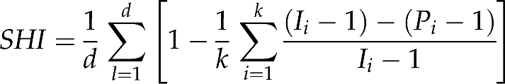where d is the number of loci in the data set, k is the number of alleles at the locus l, I_i is the number of instances of allele i, and P_i is the number of distinct mutational paths observed to lead to allele i. The expression on the right-hand side of the rightmost summation sign was set to 0 if I_i=1. SHI ranges from 0 (no homoplasy) to 1 (every allele is homoplastic). SHI was calculated for every allele, whether or not it was present in all subpopulations, making it a different quantity than the index of size homoplasy defined by Estoup et al. (2002).

Admixture

We also investigated whether sampling from a recently admixed population interfered with accurate inference of population structure. We considered an admixed population C and parent populations A and B. Population C was generated by drawing proportion p of its lineages from parent population A and proportion 1-p of its lineages from parent population B. Moving forward in time, no gene flow was allowed between populations A, B and C. Before creation of population C by admixture, we simulated no gene flow between the parent populations A and B. We varied p (0.1 or 0.5) and the time since divergence of parent populations A and B (0.15 or 0.4 N_e generations). In all cases, the admixture event occurred 10⁻³ N_e generations ago, equivalent to 1 generation ago for a population with N_e=1000 or 10 generations ago for a population with N_e=10 000. 10-STRP (SMM. θ=10) and 100-SNP data sets were used, because data sets of these marker types and size showed near identical power to detect two populations at the two divergence times tested (power ∼0.68 at 0.15 N_e generations and 1.0 at 0.4 N_e generations).

We specifically investigated the questions: (1) Do samples drawn exclusively from the admixed population appear to be drawn from two genetically divergent populations?; and (2) Do samples drawn evenly from parent population A and admixed population C appear to be drawn from 1, 2, 3 or more populations? For each set of parameter values investigated, we generated 100 simulated data sets and ran STRUCTURE for K=1 through K=5. In the case of the first question, we simulated a sample of 50 individuals from admixed population C alone. In the case of the second question, we simulated a sample of 25 individuals from parent population A and 25 individuals from admixed population C. In addition to examination of log-likelihood scores for each value of K, in the case of the second question we also extracted the inferred ancestry proportions from the K=2 output file. Based on all 5000 individuals in all 100 data sets, we calculated the percentage of individuals with minor ancestry proportions <0.05 or >0.40.

Results

Divergence time

Two-population simulations

Significant power (>0.95) to detect population structure at very recent divergence times required as many as 15 times more SNPs than STRPs. For example, obtaining power of 0.95 or 0.99 at a divergence time of 0.06 N_e generations required 1000 SNPs vs 75 STRPs (Figure 1a) and 1500 SNPs vs 100 STRPs (Figure 1b), respectively. As divergence time increased, however, the number of markers required to obtain significant power declined for both marker types. This decline was precipitous for SNPs: 97.7% fewer SNPs (35 vs 1500) were needed to obtain 0.99 power for a divergence time of 0.40 N_e generations than for a divergence time of 0.06 N_e generations. Between the same time points, 90% fewer STRPs (10 vs 100) were needed to obtain 0.99 power. At divergence times >0.40 N_e generations, small, approximately equal numbers of SNPs and STRPs were needed to achieve high power. Note that these results apply to completely isolated populations and assume constant N_e.

Figure 1.

Power of SNPs and STRPs to detect population structure. SNP and STRP curves indicate the minimum number of loci needed to detect population structure with (a) 0.95 power or (b) 0.99 power. In this and all subsequent figures, points indicate parameter combinations that were tested in simulations; points are connected by lines for ease of interpretation. Unless otherwise noted, all simulations were run under the condition of no gene flow.

Five-population simulations

For a divergence time of 0.16 N_e generations, 25-STRP data sets were the first to show marked peakedness at K=5, though other values of K were still broadly supported (Figure 2a). 100 STRP data sets showed an average rescaled ΔK of 0.98 for K=5 (values of rescaled ΔK close to 1 suggest strong support for a particular number of populations), whereas other values of K received little support (Figure 2a). 35-SNP data sets showed a bias toward low K-values (Figure 2b). Even 10 000-SNP data sets were less efficient at detecting five populations than 100 STRPs (Figure 2). However, 1000-SNP data sets in which all loci were ascertained based on the criterion of minor allele frequency >0.1 were near perfect at detecting the correct value of K (Figure 2b).

Figure 2.

Ability of SNPs and STRPs to detect five simulated populations. All simulations were simulated with a divergence time of 0.16 N_e.

Single loci and genetic differentiation

For all divergence times tested, the average SNP locus had considerably less power than the average STRP locus to detect genetic differentiation between isolated populations (Figure 3). For all divergence times >0.2 N_e generations, SNP loci showed ∼25% the power of STRP loci at the α=0.05 level. SNP loci ascertained on the basis of heterozygosity >0.2 in an ascertainment sample of five chromosomes performed better (Figure 3). However, ascertained SNP loci still only possessed ∼50% of the power of non-ascertained STRP loci at the α=0.05 level for all divergence times >0.2 N_e generations.

Figure 3.

Power of individual SNPs and STRPs. For each set of parameter values tested, 1000 SNP and 1000 STRP loci were individually tested for significant differentiation using the probability test of genic differentiation in GENEPOP. Loci used to generate the ascertained SNP were ascertained using an ascertainment sample of 25 chromosomes from one of the two populations.

Gene flow

For small data sets, power to detect the presence of structured populations was markedly reduced by a single migrant per generation (N_em=1.0). At divergence times >0.15 N_e generations, small data sets of both marker types were similarly affected by modest gene flow, showing 30–50% reductions in power (Figure 4a: 10 STRPs; Figure 4b: 100 SNPs). 25-STRP and 200-SNP data sets were less affected by gene flow at the level of N_em=1 (Figure 4).

Figure 4.

Effect of gene flow on power of SNPs and STRPs to detect population structure. The effect of one migrant per generation on the power to detect population structure for data sets comprising (a) 10 or 25 STRPs; (b) 100 SNPs.

STRP mutation

Mutation rate

Increasing STRP mutation rate by an order of magnitude (θ=10 vs θ=100; both SMM) resulted in a significant reduction in power for simulations of 15 STRP data sets under conditions of no gene flow (Figure 5a). While θ=10 data sets reached >0.90 power at a divergence time of ∼0.15 N_e generations, θ=100 data sets did not obtain >0.90 power until ∼0.30 N_e generations. When the same simulations were run using an IAM model, thereby eliminating homoplastic alleles from data sets, θ=100 data sets failed to show increased power with divergence time, whereas θ=10 data sets showed a dramatic improvement in power relative to θ=10, SMM data sets (Figure 5a).

Figure 5.

Effect of mutation rate and model on the power of STRPs to detect population structure. (a) power of 15 STRP data sets (simulated with θ=10 or θ=100) to detect population structure under IAM and SMM; (b) homoplasy as measured by SHI for θ=10 and θ=100, under the SMM, as well as θ=10 under the GSM (P=0.42) and IAM; (c) power of 15 STRP data sets to detect population structure under SMM and GSM (P=0.42). All simulations were run under the condition of no gene flow.

Homoplasy

As expected under an SMM, homoplasy as measured by SHI (Figure 5b) increased significantly with θ, plateauing at ∼0.55 for θ=100 at 0.1 N_e generations and reaching ∼0.20 for θ=10 at a divergence time of 1.04 N_e generations. For θ=10 data sets, SHI increased slightly across the entire range of divergence times tested, indicating continued accumulation of homoplasy. SHI failed to increase beyond a divergence time of 0.1 N_e generations for θ=100 data sets. The plot of SHI for GSM-modeled data sets (θ=10) closely tracked that of SMM (θ=10) data sets (Figure 5b). Thus, despite a doubling of diversity at GSM modeled loci (see the section ‘STRP mutation model'), this mutation model did not affect levels of homoplasy. As expected, IAM modeled data sets were free of homoplasy (Figure 5b), validating our method for approximating an infinite alleles mutation process at STRP loci.

STRP mutation model

GSM (P=0.42, θ=10) modeled, 15-STRP data sets outperformed SMM-modeled data sets, though the effect was only marginal for divergence times >0.15 N_e generations (Figure 5c). The number of alleles at GSM (P=0.42, θ=10) modeled loci were roughly double that of SMM loci: 17.1 and 8.3 alleles/locus for GSM and SMM loci, respectively (based on the metapopulation, averaged over 1000 simulated loci).

SNP haplotypes

15-SNP-haplotype data sets (θ=1, see Materials and methods) offered near identical performance to 15 STRP data sets in STRUCTURE analyses. Increasing marker number from 15 to 35 did less to improve the power of SNP haplotype data sets than STRP data sets (Figure 6a). The number of polymorphic loci comprising a simulated SNP haplotype varied from run to run. The average number of polymorphic loci per haplotype ranged from 5.47 to 7.04 for divergence times of 0.02 and 0.40 N_e generations, respectively.

Figure 6.

Power of SNP haplotypes. (a) Comparison of the power of SNP haplotype and STRP data sets to detect population structure using STRUCTURE. (b) Comparison of the power of single SNP haplotypes and their component SNPs to detect significant population differentiation using GENEPOP. The data points are each derived from the simulation of 1000 SNP haplotypes.

We also analyzed the power of individual SNP haplotypes and their component SNPs to diagnose genetic differentiation between populations. Figure 6b illustrates the increase in power that resulted from the combination of completely linked SNPs. For divergence times < 0.1 N_e generations, individual SNP haplotypes showed only modest improvement in power relative to the average individual SNP comprising them. For divergence times >0.15 N_e generations, however, an individual haplotype possessed roughly double the power of its average component SNP.

Ascertainment bias

In modeling ascertainment bias, we varied the size of subsamples used to ascertain loci: 5 (SNPs only), 25 or 50 samples from one of the two populations. For 15-STRP data sets, although ascertainment produced a marked increase in power relative to the use of non-ascertained data, the size of the ascertained subsample did not affect the magnitude of this increase (Figure 7a). The same was largely true of 35-SNP data sets. However, the increase in power due to ascertainment was greater for SNPs than STRPs. Also, for divergence times <0.14 N_e generations, SNP data sets based on ascertained subsamples of five showed a power increase that was 25–100% greater than data sets based on ascertainment subsamples of 25. For the same divergence times, ascertained subsamples of 50 showed a less dramatic increase in power.

Figure 7.

Effect of ascertainment bias. (a) 15-STRP data sets. The two ascertained curves are derived from ascertainment subsamples of 25 or 50 alleles from one population and are highly coincident. (b) 35-SNP data sets; (c) average heterozygosity (across 100 replicates) at STRP loci of the reference population from which the ascertainment subsample of 25 was drawn and the non-reference population; (d) same as C for SNPs, except that the ascertainment subsample was 5.

Figures 7c and d show the average heterozgyosity (across 100 replicates) for the reference population from which the ascertainment sample was drawn and the non-reference population. Although the graphs are based on data from ascertainment subsamples of 25 for STRPs (Figure 7c) and five for SNPs (Figure 7d), near identical results were obtained when different ascertainment subsample sizes were plotted. STRP ascertainment led to small differences in diversity between the reference and non-reference population: ∼7% lower heterozygosity in the non-reference population at 0.32 N_e generations (Figure 7c). SNP ascertainment, on the other hand, led to samples in which the reference population was much more diverse than the non-reference population: ∼37% lower heterozygosity in the non-reference population at 0.4 N_e generations (Figure 7d).

Admixture

Regardless of whether P=0.1 or 0.5 and whether the divergence of the parent populations occurred 0.15 or 0.4 N_e generations ago, K=1 consistently showed a significantly larger log-likelihood score when the simulated sample was drawn from the admixed population alone. The false-positive rate (the frequency at which K=2 was significant) was <0.05 for all parameter value combinations. In the case where the simulated sample consisted of equal number of individuals from the admixed population and one parent population, marker type, age of divergence and admixture proportion p all impacted the power to detect two populations in the sample (Table 2). Both 10-STRP and 100-SNP data sets had low power to detect two populations when P=0.5, though 100-SNP data sets were much better than 10-STRP data sets when the divergence time between parent populations was more ancient. Both marker types had power ⩾0.9 when P=0.1 and the divergence of the parent populations was 0.4 N_e generations ago. The generally greater power of 100-SNP data sets to detect two populations in the admixture case was accompanied by a larger fraction of individuals with minor ancestry proportions <0.05 (Table 2). Similarly, the proportion of individuals with minor ancestry proportions >0.4 was often much smaller for 100-SNP data sets than 100-STRP data sets (Table 2).

Table 2. The effect of sampling from an admixed population on inferred ancestry and the power to detect two populations.

Admixture proportion, P		Divergence time=0.15 Ne generations		Divergence time=0.4 Ne generations
		100-SNP	10-STRP	100-SNP	10-STRP
0.1	Power	0.56	0.24	0.90	0.93
	MAP<0.05	0.508	0.01	0.699	0.324
	MAP>0.4	0.347	0.596	0.041	0.085
0.5	Power	0.07	0.0	0.39	0.01
	MAP<0.05	0.035	0.029	0.047	0.023
	MAP>0.4	0.823	0.947	0.516	0.850

Abbreviations: SNP, single nucleotide polymorphisms, STRP, short tandem repeat polymorphisms

Divergence time refers to the time since the divergence of the parent populations contributing to the admixed population. MAP abbreviates the minor ancestry proportion, which is the proportion of individuals in all 100 simulated data sets with a minor ancestry either <0.05 or >0.4.

Discussion

In the context of detecting population structure, several recent studies have examined the power or informativeness of SNP, STRP and SNP haplotype loci using simulations or empirical data (Liu et al., 2005; Ryman et al., 2006; Narum et al., 2008; Smith and Seeb, 2008; Morin et al., 2009). In this study, we aimed to provide a more detailed comparison of these marker types with applicability to a wide variety of species by focusing on several factors expected to affect the ability to detect population structure. These factors included divergence time, gene flow, marker number, ascertainment bias, STRP mutation rate and STRP mutation model. Because of its popularity among empirical researchers and its ability to handle multi-locus data sets, we mainly focused on STRUCTURE analysis and scenarios where a hypothesis of population structure was not proposed. However, we also performed a limited number of exact tests (probability test of population differentiation) on individual SNP, STRP and SNP haplotype loci where population membership was specified a priori. Collectively, the results suggest that our conclusions are broadly relevant to studies both with and without explicit hypotheses of population structure.

Certainly, there are many other methods for inferring population structure. One of particular importance is principal components analysis (PCA), first introduced in this context more than 30 years ago (Menozzi et al., 1978) and today popularly implemented in the program SMARTPCA (Patterson et al., 2006). PCA offers several advantages, including the capacity to analyze variation at several hundred thousand SNPs in less than a minute and produce graphically intuitive output. The ability to efficiently analyze thousands of SNPs is especially attractive, as large data sets take hours if not days to analyze in STRUCTURE. We stress that the restriction of our simulation study to primarily STRUCTURE analysis is not meant to recommend its use over other methods. Below, we include several suggestions for empirical studies of population structure based on our results.

Time scale

When a panmictic population splits into two isolated populations, all genetic diversity found within these daughter populations is initially descended from the parent population. Unless the daughter populations sample diversity from the parent population unevenly (due to a small parent population or other biological/ecological factors), genetic data will fail to distinguish the daughter populations from one another for some period of post-divergence time. In other words, spatial but not genetic structure exists. As long as gene flow is limited, genetic structure eventually arises through changes in allele frequencies due to drift and the emergence of derived alleles in one population or another.

STRP loci in the parent population should show greater allelic diversity than SNP loci, thereby providing greater opportunity for early genetic differentiation of the daughter populations due to random drift. In addition, the high rate of STRP mutation suggests private STRP variants should appear and accumulate more quickly than new SNPs. Our results support the general expectation that the greatest power gap between SNPs and STRPs is found when divergence times are small. For divergence times <0.24 N_e generations, detection of population structure with >0.95 power requires 5–15 times as many SNPs as STRPs (Figure 1). If gene flow and other complicating factors are ignored, the superior efficiency of STRP data decays rapidly as divergence time increases; marker choice becomes nearly irrelevant for divergence times >0.40 N_e generations. Indeed, <50 SNPs are needed to detect structure with >0.95 power for divergence times >0.32 N_e generations. For populations with small N_e and short generation time, 0.32 N_e generations represent a relatively small number of years. Even for non-model organisms, the development of 50 unlinked SNP markers is a realistic objective.

Levels of homoplasy at STRP loci accumulate quickly (<0.1 N_e generations) and then do not increase greatly with divergence time for a given value of θ (Figure 5b; SMM). If the number of homoplastic alleles did increase significantly with divergence time, the number of STRP loci needed to attain high power might begin to increase at higher divergence times following the decline at intermediate time points. Instead, STRP power at divergence times greater than 0.20 N_e generations remains constant (for example, Figure 1).

The gap between the number of SNPs and STRPs needed to detect genetic structure in populations that diverged <0.1 N_e generations ago could soon become irrelevant due to advances in sequencing technology that make developing and genotyping large numbers of SNPs routine (Mardis, 2008). However, it is worth remembering that divergence times less than those sampled in our simulations (<0.02 N_e generations) are relevant to populations with large N_e or generation time (for example, 0.01 N_e generations is equivalent to 100 years for a univoltine organism with N_e=10 000). The exponential form of the SNP curves in Figure 1 suggests that detection of such recent population structure may require very large (perhaps impossible) numbers of unlinked SNPs. This corroborates a recent empirical result in maize (Hamblin et al., 2007) as well as the ‘phase change'—a threshold F_ST level, below which even tens of thousands SNPs are unable to detect differentiation—shown by Patterson et al. (2006).

Finding the true number of populations

Analysis of the ability of SNPs and STRPs to detect a specific number of populations at a divergence time of 0.16 N_e generations revealed a remarkable disparity. Whereas 100-STRP data sets unambiguously identified five populations (the true, simulated number), 10 000 SNP data sets still called the wrong number of populations with appreciable frequency (Figure 2). The high proportion of simulated SNP loci with low minor allele frequencies (∼20% singletons) contributed to this performance gap. However, we note that SNP data sets generated in two-population simulations possessed the same proportion of low frequency alleles. Yet, the discrepancy in performance between SNPs and STRPs was much smaller in magnitude in these cases (Figure 1: 35 STRPs vs 200 SNPs to obtain >0.95 power at the same divergence time of 0.16 N_e generations). SNP data sets in which singletons were eliminated during ascertainment (Figure 2b: 1000 SNPs, MAF>0.1) did much better at identifying the number of populations. Nevertheless, 1000 ascertained SNPs were required to equal the performance of 100 non-ascertained STRPs.

To explain the greater disparity between SNP and STRP power associated with increased population number, consider the probabilities that two populations isolated for x generations are differentiated to a degree detectable by some number of SNPs or STRPs, p_snp(x) and p_strp(x). Next, consider the ratio R₂=p_snp(x)/p_strp(x), which assesses the relative abilities of SNP and STRP data sets to detect two populations. If we consider five isolated populations (10 pairwise comparisons) and make the simplifying assumption that differentiation of each population pair is independent of every other pair, the relative ability of SNP and STRP data sets to detect differentiation between all populations is: R₅=p_snp(x)¹⁰/p_strp(x)¹⁰. For p_snp(x)=0.4 and p_strp(x)=0.5, R₂=0.8 and R₅=0.107. This thought experiment illustrates the compound effect of each additional population on the disparity between SNP and STRP power.

The power of individual SNPs and STRPs

Comparison of the power of individual SNPs and STRPs to detect genetic differentiation was performed using an exact probability test (Raymond and Rousset, 1995). Interestingly, while the power of an individual SNP never approaches that of an individual STRP (Figure 3), multi-locus SNP and STRP data sets show roughly equal power for divergence times >0.3 N_e generations (Figure 1). This finding indicates that some SNP loci outperform the average SNP by a large margin, which is in agreement with previous studies (Rosenberg et al., 2003; Turakulov and Easteal, 2003; Liu et al., 2005).

Gene flow

As gene flow increases, subpopulations become less genetically distinct from one another, which should make it more difficult to detect the presence of two populations. We simulated gene flow at the level of N_em=1 and quantified the effect on power to detect structure for both marker types. Declines in power associated with gene flow (∼30–50% less power; Figure 4) were reduced by modestly larger data sets (25 vs 10 STRPs and 200 vs 100 SNPs). These results support three related points: (1) at least for modest levels of gene flow (N_em<=1), adding markers reduces the negative effects of gene flow on power to detect structure; (2) power curves in Figure 1, based on completely isolated populations would shift up and to the right in response to gene flow; and (3) when certain that recently separated study populations are connected by appreciable gene flow and additional samples are not available, it is worth the effort to develop and use at least twice as many markers as suggested by Figure 1.

It may seem difficult to distinguish the degree to which declines in power are due to gene flow eroding the signal of two populations and the degree to which gene flow actually causes the null hypothesis of panmixia to become true. After all, at some threshold value of N_em, the divergent populations truly become a single, randomly mating population. However, the recovery of N_em=1 power curves in Figure 4 (25 STRP and 200 SNP) indicates that, for this level of gene flow, objective population structure still exists. The reduction in power shown by the 100 SNP and 10 STRP data sets in response to one migrant reflects the relative ineffectiveness of data sets with these sizes to detect the existing structure.

STRP mutation rate and model

STRPs show high mutation rates, frequent recurrent mutational events and potentially high levels of homoplasy. The first of these characteristics makes STRP loci attractive candidates for population structure analysis, whereas the latter two suggest caution. Although high STRP mutation rates increase expected levels of variation, the emergence of homoplastic alleles constrains variation from reaching maximum levels (Rousset, 1996). Understanding the mutation-rate-dependent effect of homoplasy on variation is of great importance to population structure analysis, since novel variation and homoplasy have opposite effects on the power of a data set to detect population structure.

Our results suggest a complicated interaction between the creation of novel variation and the generation of homoplasy. Not surprisingly, increasing θ from 10 to 100 roughly triples levels of homoplasy (Figure 5b) and decreases the power to detect population structure (Figure 5a). Unexpectedly, however, elimination of homoplasy from the data (IAM simulations) increases power when θ=10, yet causes power to crash when θ=100 (Figure 5a). Although a full understanding of this seeming paradox will require further research, we suggest one potential solution. First, consider the difference between θ=10 IAM and SMM curves. With sufficiently low mutation rates (for example, θ⩽10), the short, terminal branches of genealogies will often lack mutational events. In this case, the majority of mutations fall on long, internal branches; the absence of homoplasy (IAM) ensures that these mutations mark true relationships between samples and thereby increases power to detect relationships resulting from spatial population structure. Now, consider the difference between θ=100 IAM and SMM curves. If mutation is sufficiently common, a majority of terminal branches will bear mutations. This makes it nearly impossible to detect structure under the IAM, because terminal branch mutations will differentiate all samples from one another.

An interesting consequence of this interpretation is that homoplasy actually increases the power of θ=100 data sets. For an STRP evolving in the absence of homoplasy (IAM), a single mutation erases the connection of a lineage to all its ancestors. Each of the numerous terminal branch mutations in θ=100, IAM simulations dispossesses a lineage from the rest of the genealogy. Under the SMM, on the other hand, evolution of allele size is a random walk that oscillates about the ancestral allele size. Although mutation rate impacts the variance of changes in allele size over time in a structured population, the expected change in allele size is 0 (Moran, 1975; Pritchard and Feldman, 1996). In the short term, even high mutation rates are unlikely to allow allele state to wander too far from that of ancestral allele size. Alleles that share recent ancestors therefore have an appreciable probability of occupying the same state when finally sampled.

Empirical data suggest that STRP loci do not neatly conform to an SMM (Di Rienzo et al., 1994; Ellegren, 2000). We investigated the effect of multi-step mutation on STRP evolution and the consequences for population structure analysis. We simulated a GSM with parameters that ensured frequent multi-step mutations (P=0.42). This extreme value was used because we reasoned that any differences due to a mutational model would rarely be more severe than those observed using this value. Despite doubling the number of alleles, GSM-modeled loci showed homoplasy roughly equal to that of SMM-modeled loci (Figure 5b) and did not outperform SMM-modeled data sets by a wide margin (Figure 5c). These results are in agreement with a previous study that showed rough agreement between SMM- and GSM-derived data (Estoup et al., 2002).

SNP haplotypes

SNP haplotypes provide high variation (by summing per-site θ over many sites) with little or no homoplasy. SNP haplotypes provided power roughly comparable with that of STRP loci (Figure 6a), despite a simulated 10-fold greater mutational pressure at STRP loci (θ=10 vs θ=1). This result provides further evidence for the large negative influence of STRP homoplasy on the ability to detect structure.

The synergistic effect of combining SNPs into haplotypes is evident in Figure 6b. However, some qualifying statements are warranted. Recombination disrupts the shared genealogical history of a sequence and should therefore decrease the power of haplotypes to detect structure. Because we were focused on the role of mutation in detecting population structure, we did not model recombination. Nevertheless, the negative effect of recombination on power to detect structure must be considered if longer haplotypes are used or if the species in question is known to have a small θ:ρ ratio. In such cases, the negative influence of recombination on the power of longer SNP haplotypes to detect population structure may be quite significant. Our simulations also assumed that haplotype phase was known, thereby ignoring the error associated with assigning phase probabilistically. In this sense, our assessment of SNP haplotype power is also an overestimate. On the other hand, we coded SNP haplotypes for STRUCTURE analysis by characterizing each unique haplotype as a distinct allele. Thus, the relationships between haplotypes that differ at only one segregating site were treated the same as those between haplotypes that differ at every segregating site. Analyses that consider the distance between haplotypes (for example, haplotype networks) are likely to extract greater power from SNP haplotype data.

Ascertainment bias

Ascertainment of SNPs and STRPs for use in detection of population structure is generally biased (Rosenblum and Novembre, 2007; Vali et al., 2008). Specifically, highly heterozygous loci are expected to increase the ability to detect structure (Rosenberg et al., 2003). Our results support the practice of selecting loci with high heterozygosity for the purpose of population structure analysis. The power of SNP and STRP data sets increases dramatically when only loci with heterozygosity ⩾0.2 (SNPs) or ⩾0.85 (STRPs) are used (Figures 7a and b). Size of the ascertainment sample matters relatively little, though a small ascertainment sample may be preferable. In the case of SNPs, for example, ascertainment based on a sample of only three diploid individuals is likely to improve power to a greater degree than a sample of 10 or more individuals (Figure 7b). At least in the case of SNP data, the improvement in power largely results from the elimination of singletons, which are seldom uncovered in an ascertainment sample of 2 or 3 individuals.

An important caution regarding an intentionally biased ascertainment process is that the resultant data set may seriously compromise its use in estimating population size or the timing/size of demographic change (Wakeley et al., 2001). For example, drawing an ascertainment sample from a single subpopulation can result in the selection of loci that are highly variable in this population but not in others. In this regard, we observed a dramatic difference between SNP and STRP loci. Heterozygosities of the reference population (from which the ascertainment sample was drawn) and non-reference population differed by only ∼7% at STRP loci at a divergence time of 0.32 N_e generations (Figure 7c). On the other hand, the difference was ∼35% at SNP loci (Figure 7d). One interpretation of this result is that STRP loci highly heterozygous in the ascertainment sample indicate a high mutation rate at the locus, which will affect variability at the locus regardless of population. On the other hand, the variability showed by an SNP locus is more likely to result from a mutation that took place within the reference population in post-divergence time. Although this bias is advantageous with regard to population structure analysis, it frequently leads to the use of loci that are invariant in the non-reference population and decidedly uninformative with regards to demographic history. As most studies of population biology use genotype data for multiple forms of inference, it is important to remember this consequence of SNP ascertainment bias.

Admixture

Sampling from an admixed population is potentially misleading. For example, might we mistake a sample taken from an admixed population and one of its parent populations for one or three populations rather than two? A chief attraction of STRUCTURE analysis is that ancestry proportions of individuals are estimated. These ancestry proportions may provide clues as to whether admixture has taken place. For example, if we sample 100 individuals from a contiguous ‘population', run STRUCUTRE with K=2, and find that the inferred ancestries of most individuals lean heavily towards one inferred cluster or the other, this suggests that our sample covered two genetically distinct populations. On the other hand, if the inferred ancestries of most individuals are evenly distributed between both inferred clusters, this suggests we have sampled a single, recently admixed population. The latter scenario is exactly what we observed when we simulated a sample drawn from a very recently admixed population. Regardless of marker type, age of the divergence between parent populations, or admixture proportions, we were never misled into concluding that we had sampled from two populations.

Next, we simulated a sample consisting of the same number of individuals from the admixed population and one parent population. In these simulations, the parent populations had diverged from one another either 0.15 or 0.40 N_e generations ago. In the two-population simulations detailed above, 10-SNP and 100-STRP data sets were equally powered to detect two populations: ∼0.68 and 1.0 at these divergence times, respectively. Here, we are dealing with a more nuanced situation than the straightforward population split. One population resulting from the parent divergence is directly sampled, whereas the other parent population is only represented to a partial degree in samples from the admixed population. How does this affect power to detect two populations?

We found that the power to detect two populations is negatively impacted, sometimes dramatically so. In particular, when admixture proportion P=0.5 (equal contributions from both parent populations), 10 STRPs have no power to detect two populations (Table 2). Decreasing P to 0.1, thereby dramatically increasing the genetic contribution of the parent population not sampled, improves power to detect two populations, but it is still depressed for both SNPs and STRPs. When sampling populations from nature with little to no knowledge of recent admixture history, this may be a serious impediment to successful population structure analysis.

Why might the decline in power associated with sampling an admixed population be more severe for STRPs than SNPs? The higher variation at STRP loci may be to blame. Consider a SNP locus fixed for A in one parent population and G in the other. All members of the admixed population will initially be heterozygous A/G. If we sample from the A parent population and the admixed population, a random rise in frequency of G in the admixed population distinguishes the two populations. On the other hand, consider a STRP locus, where multiple alleles are contributed from each parent population. Here, a larger number of specific allele frequency changes are required for differentiation of the admixed population and sampled parent population. Namely, within the admixed population, alleles specific to the sampled parent population must decline in frequency whereas alleles specific to the unsampled parent population must rise in frequency. The chance that neutral evolution will by chance lead to this dichotomy of allele frequency changes is lower than in the SNP case, where a single frequency shift is required for differentiation.

Appendix

The details of many studies of population structure will not overlap with the specific evolutionary and experimental scenarios reported here. To aid researchers in assessing the power of a proposed or existing data set under scenarios of specific interest, we provide the C++ program MARKSIM. MARKSIM extends MS by enabling the user to simulate microsatellite data sets under all mutational models presented here. Simulated data sets are in output in STRUCTURE or whitespace-delimited format. SNP-based data sets—consisting of SNPs, SNP haplotypes or SNPSTRs (a composite marker consisting of a linked SNP and microsatellite)—may also be produced. In the case of SNP data, the user may also choose to output the simulated data in SMARTPCA format. MARKSIM has been tested on Mac OS X and a number of Linux distributions and is available at our laboratory website at: http://payseur.genetics.wisc.edu/resources.htm.

References

- Bowen BW, Bass AL, Soares L, Toonen RJ. Conservation implications of complex population structure: lessons from the loggerhead turtle (Caretta caretta) Mol Ecol. 2005;14:2389–2402. doi: 10.1111/j.1365-294X.2005.02598.x. [DOI] [PubMed] [Google Scholar]
- Brinkmann B, Klintschar M, Neuhuber F, Huhne J, Rolf B. Mutation rate in human microsatellites: influence of the structure and length of the tandem repeat. Am J Hum Genet. 1998;62:1408–1415. doi: 10.1086/301869. [DOI] [PMC free article] [PubMed] [Google Scholar]
- Crozier RH, Kaufmann B, Carew ME, Crozier YC. Mutability of microsatellites developed for the ant Camponotus consobrinus. Mol Ecol. 1999;8:271–276. doi: 10.1046/j.1365-294x.1999.00565.x. [DOI] [PubMed] [Google Scholar]
- Dieringer D, Schlotterer C. Two distinct modes of microsatellite mutation processes: evidence from the complete genomic sequences of nine species. Genome Res. 2003;13:2242–2251. doi: 10.1101/gr.1416703. [DOI] [PMC free article] [PubMed] [Google Scholar]
- Di Rienzo A, Peterson AC, Garza JC, Valdes AM, Slatkin M, Freimer NB. Mutational processes of simple-sequence repeat loci in human populations. Proc Natl Acad Sci USA. 1994;91:3166–3170. doi: 10.1073/pnas.91.8.3166. [DOI] [PMC free article] [PubMed] [Google Scholar]
- Ellegren H. Heterogeneous mutation processes in human microsatellite DNA sequences. Nat Genet. 2000;24:400–402. doi: 10.1038/74249. [DOI] [PubMed] [Google Scholar]
- Estoup A, Jarne P, Cornuet JM. Homoplasy and mutation model at microsatellite loci and their consequences for population genetic analysis. Mol Ecol. 2002;11:1591–1604. doi: 10.1046/j.1365-294x.2002.01576.x. [DOI] [PubMed] [Google Scholar]
- Evanno G, Regnaut S, Goudet J. Detecting the number of clusters of individuals using the software STRUCTURE: a simulation study. Mol Ecol. 2005;14:2611–2620. doi: 10.1111/j.1365-294X.2005.02553.x. [DOI] [PubMed] [Google Scholar]
- Hamblin MT, Warburton ML, Buckler ES. Empirical comparison of simple sequence repeats and single nucleotide polymorphisms in assessment of maize diversity and relatedness. PLoS ONE. 2007;2:e1367. doi: 10.1371/journal.pone.0001367. [DOI] [PMC free article] [PubMed] [Google Scholar]
- Hey J, Nielsen R. Multilocus methods for estimating population sizes, migration rates and divergence time, with applications to the divergence of Drosophila pseudoobscura and D persimilis. Genetics. 2004;167:747–760. doi: 10.1534/genetics.103.024182. [DOI] [PMC free article] [PubMed] [Google Scholar]
- Hudson RR. Generating samples under a Wright-Fisher neutral model of genetic variation. Bioinformatics. 2002;18:337–338. doi: 10.1093/bioinformatics/18.2.337. [DOI] [PubMed] [Google Scholar]
- Latch EK, Scognamillo DG, Fike JA, Chamberlain MJ, Rhodes OE. Deciphering ecological barriers to North American River Otter (Lontra canadensis) gene flow in Louisiana landscape. J Hered. 2008;99:265–274. doi: 10.1093/jhered/esn009. [DOI] [PubMed] [Google Scholar]
- Liu N, Chen L, Wang S, Oh C., Zhao H. Comparison of single-nucleotide polymorphisms and microsatellites in inference of population structure. BMC Genetics. 2005;6 (Suppl. 1:s26. doi: 10.1186/1471-2156-6-S1-S26. [DOI] [PMC free article] [PubMed] [Google Scholar]
- Marchini J, Cardon LR, Phillips MS, Donnelly P. The effects of human population structure on large genetic association studies. Nat Genet. 2004;36:512–517. doi: 10.1038/ng1337. [DOI] [PubMed] [Google Scholar]
- Menozzi P, Piazza A, Cavalli-Sforza L. Synthetic maps of human gene frequencies in Europeans. Science. 1978;201:786–792. doi: 10.1126/science.356262. [DOI] [PubMed] [Google Scholar]
- Mardis ER. The impact of next-generation sequencing technology on genetics. Trends Genet. 2008;24:133–141. doi: 10.1016/j.tig.2007.12.007. [DOI] [PubMed] [Google Scholar]
- Moran PAP. Wandering distributions and the electrophoretic profile. Theor Popul Biol. 1975;8:318–330. doi: 10.1016/0040-5809(75)90049-0. [DOI] [PubMed] [Google Scholar]
- Morin PA, Luikart G, Wayne RK. SNPs in ecology, evolution, and conservation. Trends Ecol Evol. 2004;19:208–216. [Google Scholar]
- Morin PA, Martien KK, Taylor BL. Assessing statistical power of SNPs for population structure and conservation studies. Mol Ecol Resources. 2009;9:66–73. doi: 10.1111/j.1755-0998.2008.02392.x. [DOI] [PubMed] [Google Scholar]
- Nachman MW, Crowell SL. Estimate of the mutation rate per nucleotide in humans. Genetics. 2000;256:297–304. doi: 10.1093/genetics/156.1.297. [DOI] [PMC free article] [PubMed] [Google Scholar]
- Narum SR, Banks M, Beacham TD, Bellinger MR, Campbell MR, Dekoning J, et al. Differentiating salmon populations at broad and fine geographical scales with microsatellites and single nucleotide polymorphisms. Mol Ecol. 2008;17:3464–3477. doi: 10.1111/j.1365-294x.2008.03851.x. [DOI] [PubMed] [Google Scholar]
- Ohta T, Kimura M. Model of mutation appropriate to estimate number of electrophoretically detectable alleles in a finite population. Genet Res. 1973;22:201–204. doi: 10.1017/s0016672300012994. [DOI] [PubMed] [Google Scholar]
- Patterson N, Price AL, Reich D. Population structure and eigenanalysis. PLoS Genetics. 2006;2:2074–2093. doi: 10.1371/journal.pgen.0020190. [DOI] [PMC free article] [PubMed] [Google Scholar]
- Pritchard JK, Feldman MW. Statistics for microsatellite variation based on coalescence. Theor Popul Biol. 1996;50:325–344. doi: 10.1006/tpbi.1996.0034. [DOI] [PubMed] [Google Scholar]
- Pritchard JK, Rosenberg NA. Use of unlinked genetic markers to detect population stratification in association studies. Am J Hum Genet. 1999;65:220–228. doi: 10.1086/302449. [DOI] [PMC free article] [PubMed] [Google Scholar]
- Pritchard JK, Stephens M, Donnelly P. Inference of population structure using multilocus genotype data. Genetics. 2000;155:945–959. doi: 10.1093/genetics/155.2.945. [DOI] [PMC free article] [PubMed] [Google Scholar]
- Pritchard JK, Wen X, Falush D.2007Documentation for structure software: version 2.2Accessed at: http://pritch.bsd.uchicago.edu/structure.html .
- Raymond M, Rousset F. An exact test for population differentiation. Evolution. 1995;49:1280–1283. doi: 10.1111/j.1558-5646.1995.tb04456.x. [DOI] [PubMed] [Google Scholar]
- Richards CM. Inbreeding depression and genetic rescue in a plant metapopulation. Am Nat. 2000;155:383–394. doi: 10.1086/303324. [DOI] [PubMed] [Google Scholar]
- Rosenberg NA, Li LM, Ward R, Pritchard JK. Informativeness of genetic markers for inference of ancestry. Am J Hum Genet. 2003;73:1402–1422. doi: 10.1086/380416. [DOI] [PMC free article] [PubMed] [Google Scholar]
- Rosenblum EB, Novembre J. Ascertainment bias in spatially structured populations: a case study in the eastern fence lizard. J Hered. 2007;98:331–336. doi: 10.1093/jhered/esm031. [DOI] [PubMed] [Google Scholar]
- Rousset F. Equilibrium values of measures of population subdivision for stepwise mutation processes. Genetics. 1996;142:1357–1362. doi: 10.1093/genetics/142.4.1357. [DOI] [PMC free article] [PubMed] [Google Scholar]
- Rowe G, Beebee TJC. Defining population boundaries: use of three Bayesian approaches with microsatellite data from British natterjack toads (Bufo calamita) Mol Ecol. 2007;16:785–796. doi: 10.1111/j.1365-294X.2006.03188.x. [DOI] [PubMed] [Google Scholar]
- Rubinsztein DC, Leggo J, Amos W. Microsatellites evolve more rapidly in humans than in chimpanzees. Genomics. 1995a;30:610–612. doi: 10.1006/geno.1995.1285. [DOI] [PubMed] [Google Scholar]
- Rubinsztein DC, Amos W, Leggo J, et al. Microsatellite evolution – evidence for directionality and variation in rate between species. Nat Genet. 1995b;10:337–343. doi: 10.1038/ng0795-337. [DOI] [PubMed] [Google Scholar]
- Ryman N, Palm S, Andre C, et al. Power for detecting genetic divergence: differences between statistical methods and marker loci. Mol Ecol. 2006;15:2031–2045. doi: 10.1111/j.1365-294X.2006.02839.x. [DOI] [PubMed] [Google Scholar]
- Schaffner SF, Foo C, Gabriel S, Reich D, Daly MJ, Altshuler D. Calibrating a coalescent simulation of human genome sequence variation. Genome Res. 2005;15:1576–1583. doi: 10.1101/gr.3709305. [DOI] [PMC free article] [PubMed] [Google Scholar]
- Smith CT, Seeb LW. Number of alleles as a predictor of the relative assignment accuracy of short tandem repeat (STR) and single-nucleotide-polymorphism (SNP) baselines for chum salmon. T Am Fish Soc. 2008;137:751–762. [Google Scholar]
- Taylor EB, Boughman JW, Groenenboom M, Sniatynski M, Schluter D, Gow JL. Speciation in reverse: morphological and genetic evidence of the collape of a three-spined stickleback (Gasterosteus aculeatus) species pair. Mol Ecol. 2006;15:343–355. doi: 10.1111/j.1365-294X.2005.02794.x. [DOI] [PubMed] [Google Scholar]
- Turakulov R, easteal S. Number of SNPS loci needed to detect population structure. Hum Hered. 2003;55:37–45. doi: 10.1159/000071808. [DOI] [PubMed] [Google Scholar]
- Udupa SM, Baum M. High mutation rate and mutational bias at (TAA)(n) microsatellite loci in chickpea (Cicerurietinum L. Mol Genet Genomics. 2001;265:1097–1103. doi: 10.1007/s004380100508. [DOI] [PubMed] [Google Scholar]
- Underhill PA, Kivisild T. Use of Y chromosome and mitochondrial DNA population structure in tracing human migrations. Ann Rev Genet. 2007;41:539–564. doi: 10.1146/annurev.genet.41.110306.130407. [DOI] [PubMed] [Google Scholar]
- Vali U, Elnarsson A, Waits L, Ellegren H. To what extent do microsatellite markers reflect genome-wide genetic diversity in natural populations. Mol Ecol. 2008;17:3808–3817. doi: 10.1111/j.1365-294X.2008.03876.x. [DOI] [PubMed] [Google Scholar]
- Vandergast AG, Bohonak AJ, Weissman DB, Fisher RN. Understanding the genetic effects of recent habitat fragmentation in the context of evolutionary history: phylogeography and landscape genetics of a southern California endemic Jerusalem cricket (Orthoptera: Stenopelmatidae: Stenopelmatus) Mol Ecol. 2007;16:977–992. doi: 10.1111/j.1365-294X.2006.03216.x. [DOI] [PubMed] [Google Scholar]
- Wakeley J, Nielsen R, Liu-Cordero SN, Ardlie K. The discovery of single-nucleotide polymorphisms – and inferences about human demographic history. Am J Hum Genet. 2001;69:1332–1347. doi: 10.1086/324521. [DOI] [PMC free article] [PubMed] [Google Scholar]
- Xu X, Peng M, Fang Z, Xu X. The direction of microsatellite mutations is dependent upon allele length. Nat Genet. 2000;24:396–399. doi: 10.1038/74238. [DOI] [PubMed] [Google Scholar]
- Zhang DX, Hewitt GM. Nuclear DNA analyses in genetic studies of populations: practice, problems and prospects. Mol Ecol. 2003;12:563–584. doi: 10.1046/j.1365-294x.2003.01773.x. [DOI] [PubMed] [Google Scholar]