Abstract
In this paper, we propose a coupled level set (LS) framework for segmentation of bladder wall using T1-weighted magnetic resonance (MR) images with clinical applications to virtual cystoscopy (i.e., MR cystography). The framework uses two collaborative LS functions and a regional adaptive clustering algorithm to delineate the bladder wall for the wall thickness measurement on a voxel-by-voxel basis. It is significantly different from most of the pre-existing bladder segmentation work in four aspects. First of all, while most previous work only segments the inner border of the wall or at most manually segments the outer border, our framework extracts both the inner and outer borders automatically except that the initial seed point is given by manual selection. Secondly, it is adaptive to T1-weighted images with decreased intensities in urine, as opposed to enhanced intensities in T2-weighted scenario and computed tomography. Thirdly, by considering the image global intensity distribution and local intensity contrast, the defined image energy function in the framework is more immune to inhomogeneity effect, motion artifacts and image noise. Finally, the bladder wall thickness is measured by the length of integral path between the two borders which mimic the electric field line between two iso-potential surfaces. The framework was tested on six datasets with comparison to the well-known Chan-Vese (C-V) LS model. Five experts blindly scored the segmented inner and outer borders of the presented framework and the C-V model. The scores demonstrated statistically the improvement in detecting the inner and outer borders.
Index Terms: Virtual cystoscopy, bladder wall segmentation, coupled level sets, deformable model, regional adaptive clustering algorithm, T1-weighted MR imaging
I. INTRODUCTION
According to American Cancer Society, bladder cancer is the fifth leading cause of cancer deaths in the United States, and early diagnosis of bladder abnormalities is crucial for effective treatment of bladder carcinoma [1, 2]. In addition, bladder cancer is reported to have high recurrence rate after resection of the tumors (as high as 80%) [3]. Therefore, a safe, non-invasive, easy-performance method is desired to detect bladder growth abnormality for prevention from bladder carcinoma. Currently, cystoscopy is believed to be the most accurate diagnostic procedure for bladder evaluation, despite the fact that it is invasive, expensive, and uncomfortable with limited field-of-view (FOV). Recent advances in medical imaging technologies make virtual cystoscopy (VCys) a potential alternative [4~9]. By constructing a three-dimensional (3D) virtual bladder model, the VCys mimics the navigation environment of cystoscopy and detects bladder lesion candidates for urologists’ further inspection to decide if cystoscopic intervention is necessary.
Most previous VCys work [4~9] are based on computed tomography (CT) technology, due to its high spatial resolution, fast acquisition speed, and wide availability. However, the sensitivity of CT to soft tissues (including the urine) prohibits itself from providing good image contrast in bladder wall [10]. This limitation can be partially mitigated by injection of contrast medium [8, 9, 11, 12]. Unfortunately, not only this procedure becomes invasive and uncomfortable, the CT scanning also delivers excessive X-ray exposure to the patients, both of which considerably increase the patients’ risk. To avoid these obstacles, magnetic resonance imaging (MRI) turns out to be an alternative, considering its structural, functional and pathological information for diagnosing and staging the tumor growth. Besides, it uses endogenous rather than exogenetic contrast medium to alter the image intensity of bladder wall against its surroundings (urine inside and fat outside) towards a fully non-invasive procedure [13, 14]. Since hydrogen in water (or urine) has longer transverse relaxation time leading to higher intensity value in the T2-weighted MR images, many previous MRI-based VCys or MR cystography researches focused on T2-weighted imaging [15~17], where urine is used as endogenous contrast medium to enhance the image contrast between bladder lumen and wall. Preliminary results showed that there is no statistically significant difference between MR and CT cystography for detection of tumors (sensitivity of 88.9% for tumors less than 10 mm and 100% for tumors equal or greater than 10 mm) [15~17]. Therefore, MR cystography may be a better choice for bladder evaluation.
As reported in [2], bladder carcinoma invades gradually from the mucosa into the wall muscles. Depending upon the degrees of penetration, bladder carcinoma is categorized into different stages. It is hoped that the transition at different stages can be reflected by image geometry and intensity features in the bladder wall [13, 14]. So far, geometrical analysis on the wall remains the primary tool (with some additional intensity texture information) for locating bladder lesions by some irregular shape and contrast patterns at a late stage [8, 16, 17]. At early stages, flat and/or small tumors less than 5 mm are difficult to be detected and, therefore, deserved more attention [8, 16, 17]. Conventional quantitative measurements on the bladder wall, like curvedness and shape index, vary significantly from voxel to voxel [18]. In contrast, for a small bump protruding out of the bladder wall, the measurement of its thickness as the distance between the inner and outer borders tends to be a good indicator of the occurrence of abnormalities [8, 11~14]. Towards that end, the issue of accurately delineating the bladder wall inner and outer borders arises [18~20].
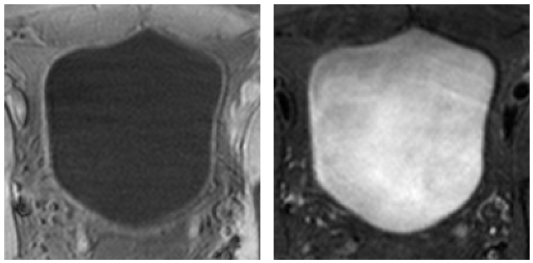
In this paper, we propose a novel segmentation approach, alternative to our previous segmentation work [18~20], to delineate the inner and outer borders. From the segmented borders, wall thickness is measured by the length of the integral path which mimics the electric field line between two iso-potential surfaces. We hope the thickness will serve as an indicator of the presence of potential bladder abnormalities, in addition to the wall geometry and texture patterns [13, 14]. Instead of following pre-existing work of focusing on T2-weighted images, we instead consider T1 imaging without exogenetic contrast medium. The reason is of two folds. On one hand, the decreased image intensities of urine in T1-weighted images provide good contrast between the bladder wall and the bladder lumen. On the other hand, the partial volume (PV) effect in T1-weighted image goes from wall toward the lumen and, therefore, is less visible, while in T2-weighted image, it goes from lumen into the wall region and can “swallow” small abnormal growth on the inner border. Typical examples of T1- and T2-weighted bladder MR images are illustrated in Fig. 1.
Fig. 1.
Typical examples of T1-weighted (left) and T2-weighted (right) MR images of the bladder. The bladder wall is more distinguishable in T1-weighted image than in T2-weighted scan.
The proposed approach is based on level set (LS) method, which is originated from geometric deformable model proposed in 1988 [21]. Early effort of using deformable model to delineate the shape of bladder from CT images has shown good results [10, 22]. In this work, we adapt the LS method to segment T1 images and explore a coupled LS framework to segment the inner and outer borders simultaneously.
The remainder of this paper is organized as follows. Section II briefly introduces the LS method and reviews its early applications in image segmentation. In section III, the coupled LS framework or pipeline for segmenting the inner and outer borders of the bladder wall is presented with details on the implementation of every building block in the segmentation pipeline. Section IV reports experimental results from patient studies with comparison to pre-existing method. Finally, section V summarizes the experimental studies and outlines our future work.
II. OVERVIEW OF LEVEL SET METHOD
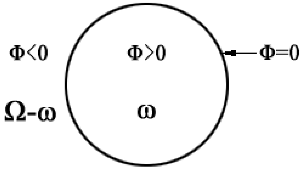
Level set (LS) method was proposed by Osher and Sethian in 1988 [21] as a geometric deformable model to implicitly describe evolving surfaces (or a curve in 2D case). Mathematically, let Ω ⊂ Rn be the data domain, an N dimensional surface S (which is the boundary of an open sub-set ω ∈ Ω, i.e., S = ∂ω) is implicitly expressed by a scalar Lipschitz continuous function (i.e., the LS function) ϕ (x1 x2, ⋯, xn) : Ω → R. The surface S is the zero LS surface (ZLSS) of the Lipschitz function when ϕ (x1 x2, ⋯, xn) = 0. This idea is illustrated in Fig. 2 by assuming n = 2. In general, the LS function is given by the signed distance function, ϕ (x1 x2, ⋯, xn) = ± d, where d is the nearest distance from x = (x1 x2, ⋯, xn) to the ZLSS and ϕ = + d in ω, ϕ = − d in Ω-ω, and ϕ = 0 on ∂ω. For simplicity, an image voxel located at x will be indicated by x in the follows.
Fig. 2.
An illustration of the level set function and the zero level set surface.
For image segmentation, LS method adds dynamics to the implicit surface. An artificial time t and force F are introduced to define the evolution of the LS function which is originated from curve evolution theory [23]. The evolution is described by
| (1) |
where F = Fimage + Fgeometry. Fgeometry is the geometry force and Fimage is the image force. Fgeometry is generated from the LS function itself to control the geometrical and topological properties of the ZLSS during the evolution. For example, Fgeometry maintains the smoothness of the ZLSS when disturbance occurs on Fimage. Fimage is generated from image information. By properly defining edge-based image force, region-based image force, or their combination, LS function evolves and finally terminates its ZLSS on the boundaries of different regions. Since the distance function is used as the LS function, i.e., |∇ϕ| = 1, then Eq. (1) is simplified as:
| (2) |
Practically, the LS function updates step-by-step according to artificial time t
| (3) |
with n ≥ 0, where ϕn is the LS function at the n-th time step. When t = 0, ϕ0 is the initial LS function.
Chan and Vese proposed a method, (C-V) model [24, 25], to utilize region-based information to construct the force. The C-V model makes Eq. (3) possible to segment regions without or with weak edges. Different from other models, the C-V model generates the force from a pre-defined energy E which consists of image and geometry terms
| (4) |
For a two-region segmentation problem, the energy is written as
| (5) |
where I(x) represents image intensity. f1 (·) and f2 (·) are either the two mean intensity values of the two regions or two continuous functions which are estimates of the image intensity I(x) of the two regions. H(ϕ)is the Heaviside function, whose value is 1 where ϕ > 0 and 0 where ϕ ≤ 0. The first and second terms together are Eimage while the third term is Egeometry, where ν is an adjustable parameter.
The associated Euler-Lagrange equations, obtained by minimizing function (5) with respect to ϕ is
| (6) |
III. COUPLED LEVEL SET SEGMENTATION ALGORITHM
The pipeline of the proposed coupled LS segmentation framework is depicted in Fig. 3. Two LS functions, i.e., inner LS function (ILSF) and outer LS function (OLSF), are used to segment the inner and outer borders of the bladder wall respectively. The bladder wall is defined as the region within the two borders. Two ZLSSs from ILSF and OLSF respectively are used to represent the two borders. The pipeline includes five steps. First of all, an initial ZLSS of ILSF is made inside the bladder lumen (i.e., Step 1). Secondly, the ILSF evolves to search for the inner border (i.e., Step 2). Considering the similarity of global shape between the inner and outer borders except for local deformed patches due to the occurrences of abnormalities, we initialize the OLSF by evolving a few iterations after Step 2 outward from the ILSF in the third step. Then, the ILSF and OLSF evolve iteratively until both the inner and outer borders are found (i.e., Step 4). Finally, based on the segmentation results, the thickness of the bladder wall is measured and rendered in a 3D virtual bladder model.
Fig. 3.
A flowchart of the coupled level set framework for bladder wall segmentation. It consists of five steps.
In the following, the coupled LS framework for segmentation of the inner and outer borders of the bladder wall is presented in details.
A. Initializing the Inner Border ILSF (Step 1)
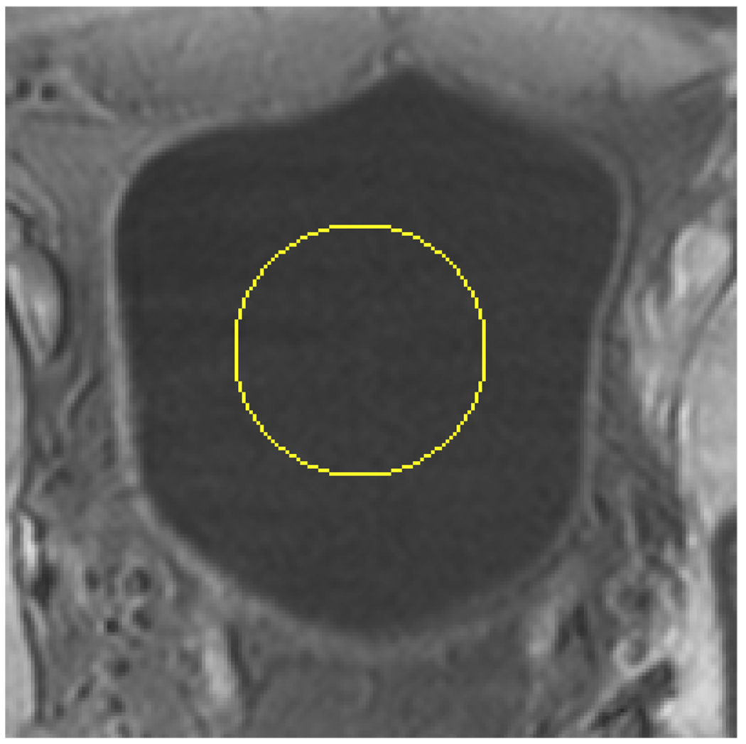
The purpose of this step is to allocate an initial ZLSS of the ILSF inside the bladder lumen so that the ILSF will evolve toward the inner border of the bladder wall. As shown in Fig. 1, the soft tissues outside the bladder in the T1-weighted MR image have similar image intensities as the urine inside bladder lumen. Furthermore, the shape and size of the bladder can vary significantly from patient to patient. Therefore, an allocation operation may encounter challenge if it is based only on the image intensity. While other means may be explored to accomplish this allocation task, we propose a simple, while effective way, to initialize the ILSF in this study. A ball-shaped surface is made manually as the initial ZLSS inside the bladder lumen as illustrated in Fig. 4. The size and location of the ball can be set via the mouse on the computer screen.
Fig. 4.
The ZLSS of ILSF is initialized manually inside the bladder lumen as the surface of a small ball. The yellow circle indicates the initialized ZLSS in this slice.
B. Searching for the Inner Border (Step 2)
As shown in Fig. 1, the inner border is easier to be distinguished than the outer border in the T1-weighted MR images because of the decreased image intensity of the urine inside the bladder lumen. Therefore, segmentation of the inner border is believed to be more reliable and capable of providing prior knowledge for the delineation of the outer border. Therefore, we segment the inner wall first. We modify the C-V model to adaptively segment the inner border. The energy function for the modified C-V model EMCV has the same form as function (4) including both image and geometry parts:
| (7) |
| (8) |
where I (x) is the image intensity at voxel x, and ϕ1 is the ILSF, clumen and cwall have similar meanings as f 1 and f 2, respectively; L > 0 is a predefined constant value; and
| (9) |
is a step function with T being a predefined constant value. μ1, ν1 and ν2 are adjustable parameters. All the functions and parameters appearing in Eqs. (7)–(9) will be discussed later after the Euler-Lagrange equations (similar to Eq. (6)) are derived.
While the image energy of (7) is designed for and will be used exclusively in the modified C-V model, the geometry energy Egeometry of (8), which maintains the smoothness of the ZLSS, is proposed for more general utility and can be combined with image energy in other models. Thus, we only apply the subscript “MCV” to the image energy . The total energy EMCV is the combination of the image energy and the geometry energy,
The associated Euler-Lagrange equations is obtained by minimizing EMCV with respect to ϕ1, clumen and cwall, respectively, similar to the operations for Eq. (6),
| (10) |
| (11) |
Equation (10) only preserves the terms related to the evolution of the ZLSS and removes other terms. The parameters f1 and f2 in the C-V model are obtained globally from the voxels inside and outside the ZLSS and now are replaced by clumen and cwall in our modified version, where clumen and cwall are the local mean intensity values determined by the voxels close to the ZLSS via Eq. (11). As shown in (11), the distance of those voxels to the ZLSS is less than L. By the definition of L > 0, the unrelated tissues far away from the inner border of the bladder wall will be excluded. The local operation will also mitigate the inhomogeneity effect. The advantage of modifying the C-V model from global to local operation in the image energy function is seen.
The second and third terms in (10) are derived from Egeometry. By setting μ1 to be negative constant value in the second term, the ZLSS expands outwards step-by-step. The third or last term plays the role of controlling the smoothness of the ZLSS. This can be explained by a 2D slice from the 3D T1-weighted image data in Fig. 5. We call the last term as the bent rate which has the similar function as the curvature term in Eq. (6), which is widely used in most previous LS methods. As shown in Fig. 5(d), the bent rate is generated from a disk-shaped region with radius T = 10 in implementing K (y–x)of (9), where x indicates the location of the central voxel of red color and y indicates the location of any voxel inside the disk. Thus, the last term in (10) measures the area difference between the regions (ϕ1 (y) – ϕ1 (x)) > 0 and (ϕ1 (y) – ϕ1 (x)) ≤ 0 inside the disk. The two regions are separated by the iso-curve S which consists of all voxels y where ϕ1 (y) = ϕ1 (x). By setting ν1 = ν2, the bent rate term prevents the iso-curve from over bended since the minimum energy comes from the condition that S equally divides the disk. In the 3D case, the surface S is ZLSS which means ϕ1 (x) = 0.
Fig. 5.
An example to illustrate the improvement of the bent rate against the curvature term. Picture (a) shows the original T1-weighted MR bladder image, where yellow curve is the ZLSS of ILSF. The area inside the white square frame contains 23×23 image pixels, which is enlarged in the following illustrations. Picture (b) shows the 23×23 array with the center pixel being marked red. In picture (c), the effective region of curvature is colored blue while the central pixel is colored red. In picture (d) as an example, the effective region of bent rate is a disk-shaped region with radius equal to 10 whose boundary is shown in blue. The red pixel is at the center.
Comparing with the curvature, which only takes the first order neighborhood into account, the bent rate utilizes an effective region which varies depending on the radius parameter T. In Fig. 5(c) and Fig. 5(d), we depict the effective regions for calculating the curvature and the bent rate respectively. The blue pixels in Fig. 5(c) construct the effective region for the curvature, while in Fig. 5(d) all voxels on and inside the blue circle contribute to the calculation of the bent rate. In the presence of image noise, the curvature term in (6) is more sensitive to the noise because of the limited effective region, while the last term in (10) is more immune to the noise because of the variable effective region. In the example of Fig. 5, the ZLSS bends smoothly, leading to a very small curvature value at the central pixel. This trend can be captured by the integral operation (of generating the bent rate) in a larger scale space. This is an advantage of the modified C-V model (8) over the geometry term in the original C-V model (5).
C. Initializing the Outer Border OLSF (Step 3)
This step aims to generate a reasonable initialization for OLSF (as represented by ϕ2) whose ZLSS is hoped to be not too far away from the outer border. To achieve that goal, we adapt the geometry force derived in (10), i.e., the second and third terms in (10), to evolve for an initial ZLSF of OLSF by:
| (12) |
Based on the assumption that the outer border has roughly a similar global shape as the inner border, then μ2 is designated to be a negative constant value which expands the ZLSS outward step-by-step, and a similar bent rate is implemented in this initialization procedure, where ν3 and ν4 are both positive constants corresponding to ν 1 and ν 2 in (10). As many other edge-based LS methods do [23], a stop term is used to terminate evolution at the outer border. Since the image intensity of the bladder wall is generally brighter in T1-weighted images than its surroundings, the term I (x) on the numerator makes the evolution faster inside the bladder wall than in any other place. ∇I(x) is the image gradient, and becomes a small value when the ZLSS encounters the outer border where exists prominent intensity variation. When t = 0 at the beginning of the evolution, we have ϕ2 = ϕ1. When the reaches a pre-defined small threshold, we achieve the initialization task for OLSF.
D. Segmenting the Inner and Outer Borders Iteratively (Step 4)
In this step, we construct a new image energy which will be used by both ILSF and OLSF to segment the final inner and outer borders of the bladder wall iteratively. The major idea is to use a regional adaptive clustering algorithm (RACA) to classify the voxels in a region of interest (ROI) into three groups and further to use the clustered result to construct image energy for the LS function evolution. In 1992, Pappas [26] proposed an adaptive clustering algorithm (ACA) for segmentation of images and enhancement of features based on the k-means clustering method. It assumes the intensity distribution in a region follows the Gaussian functional. Different from the k-means method in which samples in a region has one mean and one standard deviation value, the ACA divides an image into sub-windows and the voxels belong to a region but in different windows have different mean and standard deviation values. By decreasing the window size step-by-step, the ACA generates improved clustering results than the k-means method. In our RACA model, the Gaussian distribution and the window sub-dividing strategy are inherited. The differences are three fold. Firstly, a ROI around the bladder wall is specified to eliminate unrelated voxels and reduce calculating complexity. Secondly, the initial condition is not from k-means but the two LS functions (i.e., ILSF and OLSF). The last but not least important, an a priori intensity is obtained, based on the OLSF and ILSF, and is used for the classification. The details are given below.
D.1. Definition of Region of Interest
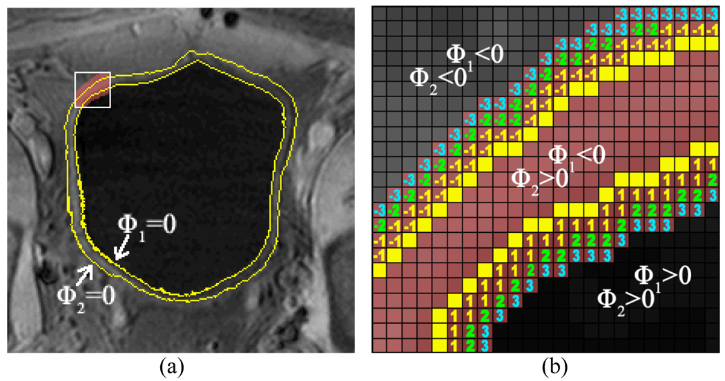
To eliminate redundant information and reduce computing time, a ROI shall be defined within which the RACA is applied. Since the ZLSSs of the ILSF and OLSF have been placed by the above Steps 2 and 3 near the inner and outer borders of the bladder wall respectively, ϕ1 and ϕ2 now roughly divide the image into three parts: bladder lumen where ϕ1 > 0 and ϕ2 > 0, bladder wall where ϕ1 < 0 and ϕ2 > 0, and soft tissues outside bladder wall where ϕ1 < 0 and ϕ2 < 0. By defining d > 0, the ROI is constructed as a band-shaped area around the bladder wall with any voxel at location x inside the ROI having ϕ2 (x) ≥ − d and ϕ1 (x) ≤ d. As shown in Fig. 6(a), the yellow curves are the ZLSSs in this slice. For illustration purpose, the area in the white frame in Fig. 6(a) is enlarged and shown in Fig. 6(b). We take d = 3 for an example. The positive and negative numbers are the values of ϕ1 and ϕ2 respectively at the corresponding voxels. The ROI inside the white frame is defined as the space which includes those voxels between the ZLSSs and also those voxels labeled −3, −2, −1, 1, 2 and 3.
Fig. 6.
An illustration of the ROI. Picture (a) shows the original image with ZLSSs in a slice. The yellow curves are the ZLSSs in this slice. Picture (b) is the enlarged region in the white frame in (a). When d = 3 is chosen as an example, the ROI in the white frame includes those voxels which are colored pink, i.e., the ROI includes (1) the space between the yellow lines and (2) the expanded space labeled −3, −2, −1, 1, 2, and 3.
D.2. Statistical Models in the Regional Adaptive Clustering Algorithm
Given the ROI, our goal is to segment those voxels inside the ROI into three regions by maximizing the a posteriori probability p(ω|I), where I represents the observed image intensities of those voxels and ω = 1, 2, 3, indicating the three region labels which are bladder lumen, bladder wall, and soft tissues outside the bladder wall respectively. By Bayes’s law, we have
| (13) |
where p (I|ω) is a Gaussian-distributed probability density function of I, conditioning on region ω with mean μω and standard deviation σω. Considering the influence from image artifacts (such as inhomogeneity effect) and more than one tissue type outside the bladder wall, we use μωx, x and σωx, x to statistically characterize each voxel at location x instead of using the global parameters μω and σω, i.e.,
| (14) |
To model the a priori probability density function P (ω), we refer to the ILSF and OLSF. As mentioned above, the ZLSSs are located nearby the bladder wall borders and, therefore, they can provide prior knowledge for the clustering procedure. A functional form of P (ω) can be
| (15) |
where ωLS,x is the LS-determined region label of voxel at location x and can be understood by the following example. As shown in Fig. 6(b), ϕ1 and ϕ2 divide the ROI into three regions, and ωLS,x denotes one of the three regions. All voxels at locations x inside the same region have the same label ωLS,x. Notation ωx is the region label of voxel at location x and is obtained by the use of the RACA, i.e., finding the mode of the posterior (13). α1 and α2 are positive constant values. The term |ωx − ωLS,x| in (15) encourages the region label ωx of voxel at location x to have the same label as its initial ωLS,x (given by the ZLSSs). The term min (|ϕ1 (x)|,|ϕ2 (x)|) is the distance from x to the nearest ZLSS. It aims to consider the uncertainty of the classification for those voxels around the boundaries. In other words, the closer the voxel at location x to one of the ZLSSs, the likely it may change class label. The last term V (ωx) in (15) is a potential, coming from the 26-connected neighbors of voxel at location x, which is defined as follows:
| (16) |
where Nx is the set of neighboring voxels. This term encourages the continuity in terms of region labels between central voxels and its neighbors. Combining the likelihood (14) and the a priori density (15), the a posteriori density p (ω|I) of (13) is rewritten as:
| (17) |
D.3. Segmentation Procedure for the Bladder Wall
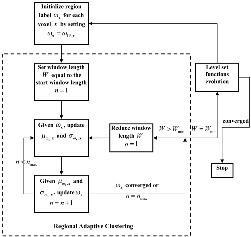
The overall flowchart of the iterative process between constructing the energy functions (via performing the RACA) and evolving the LS functions of ILSF and OLSF for the inner and outer borders of the bladder wall is depicted by Fig. 7. In each iteration cycle, the ILSF and OLSF provide prior knowledge to initialize the voxels’ region label for the RACA while the clustered results are used to generate energy functions for the evolution of the LS functions.
Fig. 7.
The flowchart which illustrates the iterative procedure of image energy construction by the use of the RACA and the LS function evolution.
In this section, we discuss three issues: (i) an algorithm to estimate the local mean μωxx and local standard deviation σωxx in the posteriori probability density function p (ω|I); (ii) given μωxx and σωxx, the estimation of the region label ωx of each voxel at location x in the ROI; and (iii) the use of the clustered results to construct the energy functions for ILSF and OLSF evolution. We briefly discuss the first and second issues because their details can be found in [26], and pay more attention to the third issue.
D.3.1 Estimation of Parameters in p (ω|I)
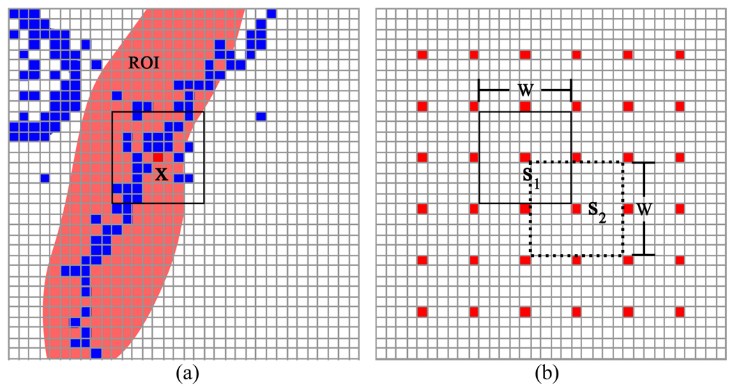
The μωxx and σωxx are estimated for each voxel at location x while the region label ωx is known. As shown in Fig. 8(a), a square window is centered at x. All voxels with the region label ω = 3 are colored blue. The ROI is highlighted by pink. Only those voxels located inside the ROI and those voxels inside the square window with exactly the same region label ω = 3 are considered for estimating the local mean μω=3,x and standard deviation σω=3,x for the central voxel x. Furthermore, instead of estimating the local mean and standard deviation for all voxels, the estimation is performed for a group of spatially-separated voxels in order to eliminate redundant information and reduce calculating burden. The performance procedure is illustrated by Fig. 8(b). The voxels in red color are samplers. The two squares outlined by the solid and dash lines are two windows with length W. s1 and s2 are two sample voxels which are also the central voxels in the windows. The distance between two adjacent sample voxels on each dimension is W/2. After the mean μω=3,x and standard deviation σω=3,x for those sampled voxels are obtained, the estimation of these two parameters for the remaining voxels is determined by linear interpolation from the samplers.
Fig. 8.
An illustration of the method for selection of sample voxels and windows to estimate the parameters for each voxel. In picture (a), only the blue voxels in the ROI and the square window are used to estimate the mean and standard deviation for the sampler voxel at location x. Picture (b) shows the discrete sampling and the window alignment.
D.3.2 Update of Region Label for Each Voxel
Given the mean μωx,x and standard deviation σωx,x for voxel at location x, the region label ωx is estimated by maximizing the a posteriori probability p(ω|I) of (13). Since global maximization of (17) is complex and time consuming, instead we maximize the conditional probability density for each voxel at location x by:
| (18) |
In other words, while the observation Ix is known and the current region labels of all other voxels are given (by the ZLLSs), we maximize p(ωx|Ix) to update ωx. For example, if p(ωx = 1|Ix) = max (p(ωx = 1|Ix),p(ωx = 2|Ix),p(ωx = 3|Ix)), then voxel at location x belongs to region 1 which is ωx =1. The maximization operation is performed voxel-by-voxel throughout the whole image. This cycle is repeated until a convergence is achieved where the number of voxels, which changed their region labels in one cycle, is less than one tenth of the total voxel number. The sub-optimum result is obtained by the greedy algorithm [27].
As shown in Fig. 7, the operations in the dotted-line box illustrate the clustering procedure of the RACA. It always starts by labeling every voxel in the ROI according to the current ILSF and OLSF condition, i.e., ωx = ωLS,x. An iteration includes one update of μωx,x and σωx,x and one update of ωx. The iteration terminates when the update of ωx converges or the maximum iteration number is reached. Then the window length is cut to half and the algorithm repeats itself until the above stopping rule is satisfied one more time. The RACA finishes when the lower bound of the window width is reached. It should be noted that a higher and a lower bound for the window width is predefined.
D.3.3 Energy Function Construction and Level Set Evolution
After the region labels of ωx are updated by the RACA above, the LS energy functions can be generated from the clustered results to evolve both the ILSF and OLSF to update the classification of the inner and outer borders. The energy can be constructed as follows:
| (19) |
where ωx = 1,2,3 have been used to represent voxel at location x in the bladder lumen, bladder wall, and soft tissues outside the bladder wall respectively. The first three terms in (19) are the image energy function while the last two terms are geometry energy function. The image energy is the integration of probability of voxels belong to region i, where i = 1,2,3. The notations in the geometry energy have the same meaning as those in (8). ν5 and ν6 are adjustable parameters with the same meanings as νi, i=1,2,3,4, as defined before.
The associated Euler-Lagrange equations, obtained by minimizing ERACA with respect to ϕ1 and ϕ2, are:
| (20) |
| (21) |
By the implementation of (3), the ILSF and OLSF evolve several time steps according to (20) and (21) until meeting the stop criteria, which is stated as that the number of updated voxels on the ZLSS is less than one tenth of the total voxel number on the ZLSS within one time step or a preset maximum iteration account is reached.
In summary, the segmentation procedure for the bladder wall is an interleaved iterative operation consisting of two iterative processes. It starts by the initial ZLSFs of Sections A–C above. From the ZLSFs, one iterative process initializes the labels for the voxels inside the ROI of the ZLSFs and updates the labels until a convergence is reached. Then another iterative process constructs new LS energy functions from the updated labels and evolves both the ILSF and OLSF until a convergence is reached. The resulted ZLSFs become the new initial to trigger next interleaved iterative operation of the two iterative processes. The interleaved iterative operation terminates for the final result under the following condition. Once after the RACA, if both the ILSF and OLSF meet their stop criteria by only evolving one time step, then the interleaved iterative operation stops and the final segmentation result is obtained.
IV. RESULTS
Six patient datasets were used to test the above presented coupled LS-based segmentation algorithm. After informed consent, these six patients were scanned by either a 1.5 Tesla or 3.0 Tesla scanner using parameters as shown in Table I. Considering the non-isotropic resolution in these T1-weighted images, the slice thickness in each dataset was interpolated to match the in-plane voxel size for cubic voxel array before performing segmentation.
Table I.
Data Information and Image Acquisition Parameters
| Dataset | Magnetic Field Strength (T) |
Scanning Protocol |
Slice Thickness (mm) |
Pixel (mm) | TR (ms) | TE (ms) |
|---|---|---|---|---|---|---|
| 1 | 3.0 | 3DFFE-SPIR CLEAR |
1.5 | 0.5804 | 4.6666 | 2.2766 |
| 2 | 3.0 | 2500 FULL SCAN CLEAR |
1.5 | 0.5804 | 4.6747 | 2.2818 |
| 3 | 3.0 | 3D 25 MIN CLEAR |
1.5 | 0.5804 | 4.6679 | 2.2756 |
| 4 | 3.0 | MPR COR | 2.0 | 0.5804 | 4.6679 | 2.2756 |
| 5 | 1.5 | THRI PELPRE SENSE |
1.75 | 0.7383 | 4.3896 | 2.1181 |
| 6 | 3.0 | 3DFFE-SPIR CLEAR |
1.5 | 0.5804 | 4.6668 | 2.2768 |
By surveying these T1-weighted MR images acquired with various parameters in the scanning protocol, we found several challenges in segmentation of the bladder wall. First of all, these T1 imaging protocols have not yet provided excellent contrast for the bladder wall against its surrounding soft tissues, although the contrast between the urine and the wall is very good. In fact, the connecting muscles to the bladder (and the adjacent prostate in male) have a similar T1 relaxation and in consequence a similar image-intensity value to the bladder wall. Secondly, the acquired images suffer from noise and artifact. Thirdly, the intensity value of the bladder wall varies from slice to slice and also in different locations within one slice due to inhomogeneity effect. Despite these challenges, the presented segmentation algorithm has shown satisfactory performance, and is expected to perform better for improved image quality as the MRI imaging technology would have been improved in the future. In the following, several investigations on the segmentation algorithm are reported.
A. Advantages of the Bent Rate over the Curvature Merit
As mentioned in section III, the bent rate is proposed in this paper to replace the traditional curvature term in the previous work [23]. Similar to the curvature, the bent rate aims to prevent the ZLSS over-bended or leaking out of small “gaps”. However, the bent rate directly takes advantage of the signed distance function, ϕ(x1,x2, ⋯, xn) = ± d, to estimate the “bent level” of the ZLSS. Furthermore, the bent rate is generated from an effective region which varies depending on the radius parameter T, while curvature only takes the first order neighbors into account. The effect region makes the bent rate more adaptive to the T1-weighted MR images.
Fig. 9 is an example illustrating the difference between the curvature and the bent rate. Fig. 9(a) shows a lesion protruding to the lumen from the inner border of the bladder wall. The occurrence of the lesion leads to a concave ZLSS of the ILSF. In step 3 or section III.C, the OLSF is initialized based on the ILSF. The influence of the concave deformation is expected to be smoothed out on the initialized ZLSS of the OLSF. Fig. 9(b) and (c) show the initialization results by the use of the curvature and the bent rate respectively. By setting T=8 and ν3 = ν4 = 10, the ZLSS of the OLSF approximates closely to the outer border of the bladder wall by the use of the bent rate as shown in Fig. 9(c). If the bent rate in (12) was replaced by the curvature term and the parameters ν3 and ν4 remained the same of 10, the generated initialization result is shown in Fig. 9(b). Because of its relatively smaller effective region (i.e., fixed to the first-order neighbors), the curvature could not flatten the concave surface for the initialized ZLSS of the OLSF.
Fig. 9.
An example which shows the influence of the bent rate and the curvature on the initialization of the OLSF. The bent rate is able to effectively flatten the concave surface and gives a better approximation for the outer border than the curvature. Picture (a) is the original image slice. Picture (b) shows the initialization of the OLSF by the use of the curvature. Picture (c) shows the initialization of the OLSF by the use of the bent rate.
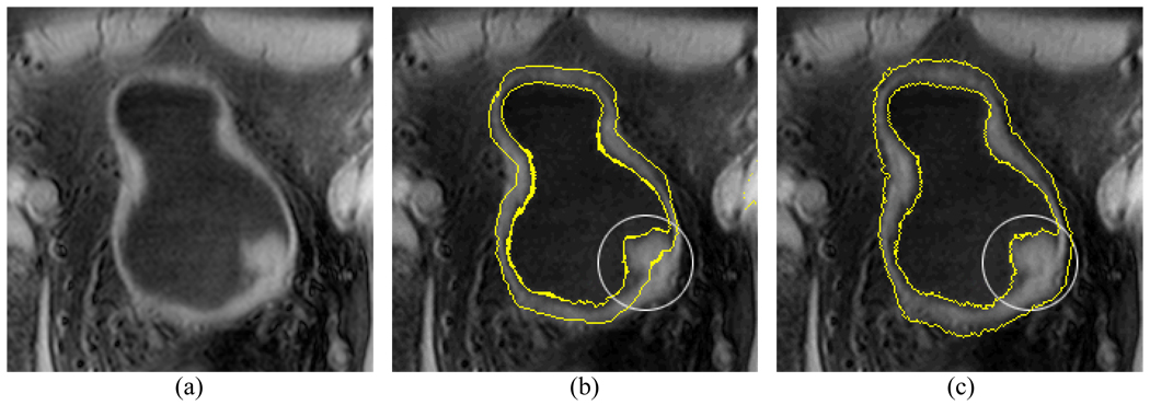
Another advantage of the bent rate is its capability of preventing the ZLSS from leaking out a weak/thin wall area. As shown in Fig. 10(a), the circled weak wall area has several voxels with noticeably decreased image intensities (due to PV effect), and the decreased intensities cause a connection between the bladder lumen and the outside adjacent tissues because they have similar intensities. In Fig. 10(b), the curvature failed to “detect” this leakage. The bent rate effectively prevented the leakage with T=8, and ν1 = ν2 = 10, as shown in Fig. 10(c).
Fig. 10.
An example which shows the difference of the bent rate and the curvature in preventing ZLSS from leaking out. The bent rate is more controllable and effective than the curvature in preventing leaking. Picture (a) is the original image slice. There is a small gap (due to decreased image intensities) as indicated by the white circle. Picture (b) shows the segmentation result by the use of the curvature. Picture (c) shows the segmentation result by the use of the bent rate.
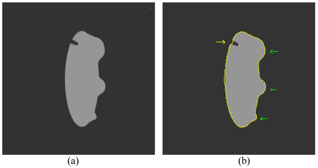
One interesting issue would be whether the bent rate will influence the segmentation of an abnormality. Based on all the studies in this work, the bent rate has little influence on the detection of abnormalities on the inner border. The bent rate could affect the results more if there is not enough contrast information. Since the image contrast is good around the inner border, the bent rate has little influence on segmenting abnormalities on the inner border. It mainly ensures the smoothness of the ZLSS of the outer border where the image contrast is relatively low. Fortunately the abnormalities always grow from the inner border of the bladder wall. If the inner border is segmented satisfactorily and the ZLSS keeps smooth around the outer border where there is less image contrast, the wall thickness would be an effective indicator to reflect the geometry changes on the inner border, including the flatter tumor. This idea is illustrated in Fig. 11.
Fig. 11.
An artificial image mimics the bladder wall which shows how the bent rate influences the segmentation result. (a) The original image. (b) The segmentation result. The yellow curve represents the segmentation result. The abnormalities of different sizes on the inner border are pointed by green arrow, while a gap on the outer border is pointed by yellow arrow.
Assume the gray region is a section of bladder wall and the interface between the gray region and the black background separates the inner and outer borders. By setting proper ν1 and ν2 values, the gap on the outer border is smoothed while the protrusions on the inner border of different sizes are segmented. Thus, the smoothing procedure has little influence on the final wall thickness measurement.
B. Comparison with the Original C-V Model
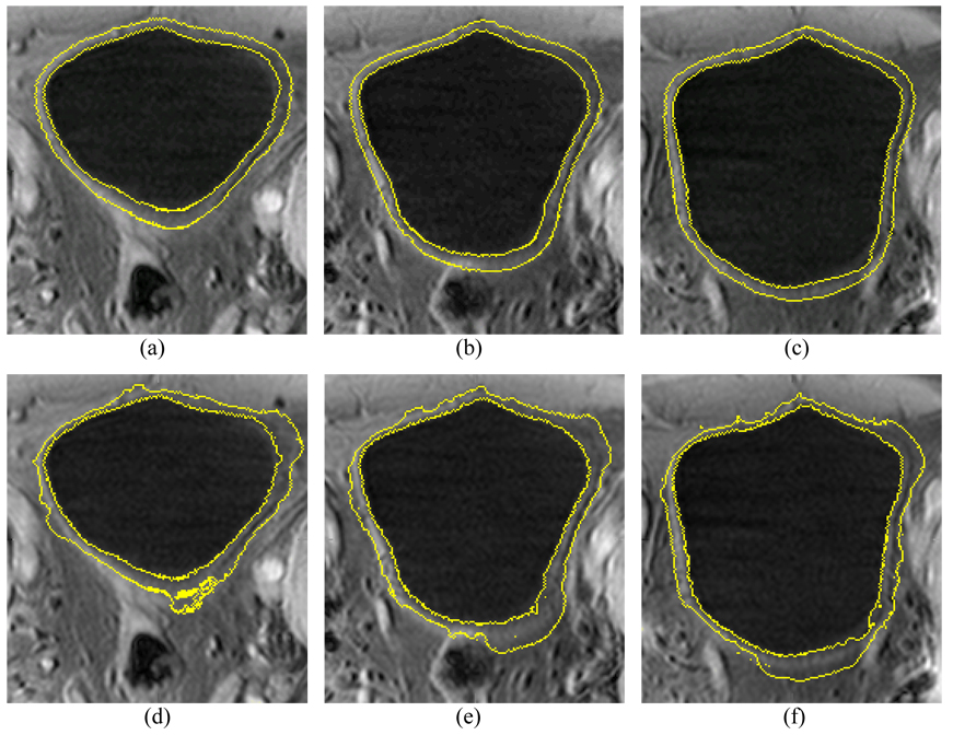
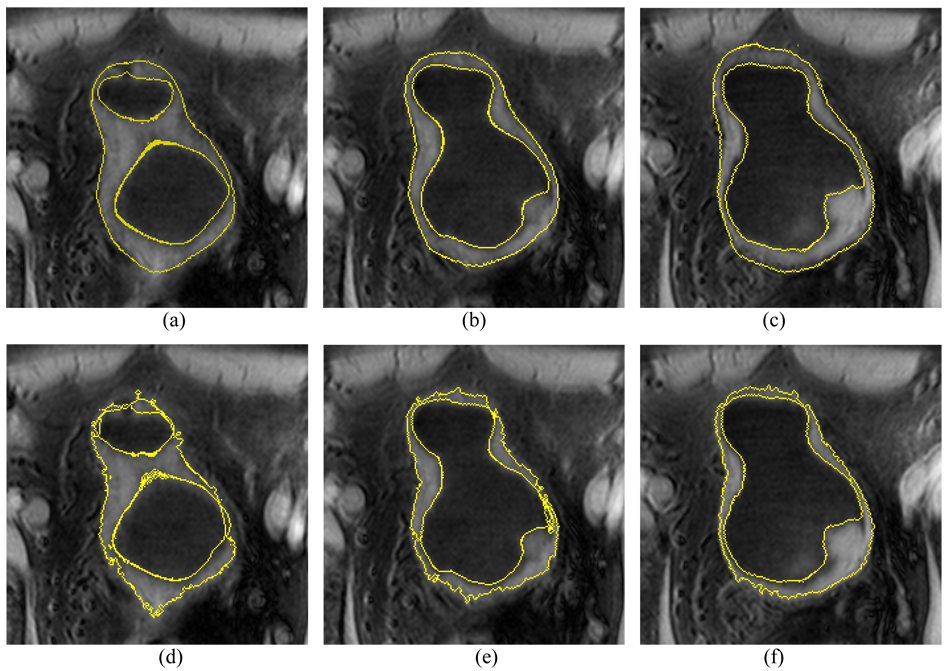
The first three steps in section III, i.e., sections III.A–C, are the same for the presented method and the original C-V model, where each method uses its terms as defined in the associated equations. The results after the third step (i.e., step 3 or section III.C) are used as the initial ILSF and OLSF. Starting from step 4, the scheme proposed in [25] was implemented for the C-V model, while the described details in section III.D above was implemented for the presented method. Their final results are compared in Fig. 12 and Fig. 13 which depict a volunteer case and a patient case respectively.
Fig. 12.
An example of segmentation results from the volunteer datasets using the presented method and the C-V model. Top row (a)–(c) shows the segmented results of the presented method. Bottom row (d)–(f) shows the segmented results of the C-V model. The intensity distribution is very complex around the outer border of the bladder wall. Since it considers the local contrast and applies prior geometry constraint, the presented method performs much better than the original C-V mode.
Fig. 13.
An example of segmentation results from the patient datasets using the presented method and the C-V mode. An abnormal protrusion is included in the slices. Pictures (a)–(c) show the segmented results of the presented method. Picture (d)–(f) show the segmented results of the C-V model. The presented method produces better results than the C-V model.
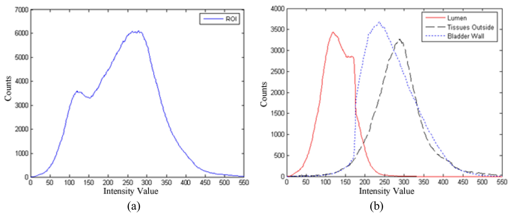
To understand their different performances, we examined the histogram properties of a volume of interest (VOI), which was obtained by enlarging the segmented outer border of Fig. 12(c) in three dimensions to include a similar amount of surrounding tissues as that of the bladder wall. Fig. 14(a) shows the histogram from the VOI. The histogram depicts the intensity distribution of the bladder lumen, bladder wall, and soft tissues outside the bladder in the VOI. The intensity distributions of the bladder wall and the surrounding soft tissues overlap on a large portion of the histogram. The C-V model only takes the global intensity information into account and neglects the local contrast. Without using the prior knowledge and the geometry constraint as discussed in step 4 above, the C-V model could not be able to produce a satisfactory segmentation between the wall and the surrounding soft tissues. Fig. 14(b) shows the histograms of the segmented bladder lumen, wall, and surrounding soft tissues respectively in the VOI. By the use of the prior knowledge and the geometry constraint as discussed in step 4 above, the presented method improved noticeably the segmentation between the bladder wall and its surrounding soft tissues.
Fig. 14.
Histogram of voxels inside a VOI enclosing the whole bladder of Fig. 12. Picture (a) is the histogram of all voxels inside the VOI. Picture (b) shows the histograms of the segmented voxels inside the VOI as bladder lumen (red), bladder wall (blue), and soft tissues outside the bladder wall (black). The image intensity distributions of the bladder wall and the surrounding soft tissues overlap on a large portion of the histogram.
C. Evaluation of the Segmented Results
To more quantitatively evaluate the difference between the presented coupled LS method and the C-V model, five experts were asked to score on the segmented results of the two methods. The segmented results were randomized in order and displayed in computer screen without any indication of which method was used for the displayed result, i.e., this is a blind procedure that the experts did not know which method was used for each displayed result. Each expert scored from 0 (worst) through 10 (best) on the segmented inner and outer borders separately for each displayed result.
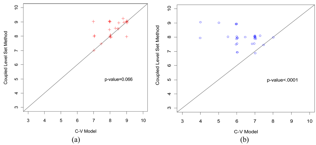
The scores from the five experts on the segmented results from the six patient datasets using the two segmentation methods were compared. The pair-wise scatter plots of the scores are illustrated in Fig. 15 for comparison of the coupled LS method against the C-V model. The scatter plots used a Jitter plot technique, which allows multiple observations with the same plotted values to be observable on the plot by adding a small amount of random noises to the values [28]. Fig. 15(a) shows the scores on the segmented inner border. Among the 30 pairs of scores, there are 13, 16, and 1 pairs that the coupled LS method was given greater, equal, and smaller scores than the C-V model, respectively. Fig. 15(b) shows the scores for the segmented outer border. Among the 30 pairs of scores, there are 27, 3, and 0 pairs that the coupled LS method gave greater, equal, and smaller scores than the C-V model, respectively. Since most of the data points fall above the 45 degree concordance line in the scatter plots, it can be concluded that the coupled LS method gets higher scores than the C-V model and, therefore, has a better performance.
Fig. 15.
Scatter plot of the scores from the coupled-LS method against the C-V model. Picture (a) shows the scatter plot of the scores from the segmented inner border. Picture (b) shows the scatter plot of the scores from the segmented outer border. The coupled-LS method gained significant higher scores than the C-V model, especially for the outer border of the bladder wall.
In addition to the Jitter plots of Fig. 15, the scores were also analyzed using a liner mixed-effects model that includes nested random effects [29]. The random effects include a random patient effect and a random border effect nested within patient. These random effects help account for the correlations between evaluation scores from the same patient and border. Fixed effects include three main effects of expert, border and method, and one interaction effect of border-by-method. This statistical analysis generated the p-values as shown in Fig. 15. The coupled LS method generated highly-significant higher score than the C-V model for the segmented outer border (p<0.0001) and approaching statistically significant for the segmented inner border (p=0.066). As discussed above, the T1-weighted images provide excellent image intensity contrast between the urine and the bladder wall for segmentation of the inner border and the C-V model mostly relies on the intensity information. Therefore, the C-V model produced comparable segmentation results for the inner border. Since the image contrast between the wall and its outside surrounding soft tissues varies noticeably, the coupled LS method obviously outperformed the C-V model on the outer border segmentation. The corresponding differences between these two methods and their 95% confident intervals are 0.33 (−0.02, 0.68) and 1.63 (1.28, 1.98) for the inner and outer borders, respectively. The expert effect is not statistically significant (p=0.37) and it seems that the variability due to different experts is relatively small and the scores from the five experts are consistent.
D. Comparison with Manually-Drawn Results
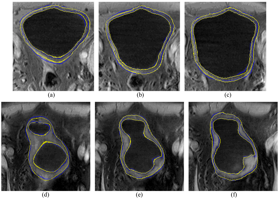
Besides the scoring evaluation above, we also conducted a comparison study with expert’s manually-traced results. An experienced radiologist was asked to outline the borders of the volunteer and patient datasets without knowing the computer-segmented results. The inner and outer borders of the bladder wall were manually drawn first, and then all voxels belonging to the bladder lumen, bladder wall and region outside the bladder were labeled respectively. Therefore, the voxel-to-voxel comparison with the presented method becomes possible. Fig. 16 shows the same cross sections of the segmentation results in Fig. 12 and Fig. 13. The blue contours were manually drawn while the yellow ones were generated by the presented computer method. Table II documents the quantitative measures on a voxel-to-voxel comparison fashion, where the merits are defined below.
Fig. 16.
Examples of manually-drawn results and computer segmentation results. Top row (a)–(c) shows the results from a volunteer study, where the blue contour represents the manually-drawn result and the yellow contour represents the computer segmentation result of the presented method. The computer segmentations results were also shown in Fig. 12 and Fig. 13. The bottom row (d)–(f) shows the results from a patient study.
Table II.
Comparison of Results from Manual and Computer Segmentation Methods
| Dataset | Minner | Mouter | AMinner | AMouter | STDinner | STDouter |
|---|---|---|---|---|---|---|
| 1 | 0.40695 | 0.23106 | 0.99313 | 1.3715 | 1.31430 | 1.7118 |
| 2 | −0.10519 | −0.76270 | 0.80906 | 1.7457 | 1.06280 | 2.0585 |
| 3 | −0.12141 | −0.51973 | 0.99544 | 2.1131 | 1.28270 | 2.6218 |
| 4 | 0.45903 | 0.70450 | 0.85647 | 2.2921 | 0.99261 | 2.7936 |
| 5 | −0.80696 | −0.71221 | 1.17930 | 1.4607 | 1.28970 | 1.7577 |
| 6 | −0.17684 | −1.44920 | 1.24170 | 1.9968 | 1.61380 | 1.8915 |
By defining di as the shortest signed distance from the ith voxel on the border segmented by the presented method to a voxel on the manually-traced border, we have three merits to quantify the difference of the computer results from the manual results:
| (22) |
| (23) |
| (24) |
From Table II, we can see that the segmentation by the presented method is similar to that of the manual procedure with approximately one voxel error. The contour generated by the computer method “oscillates” around the manually-traced contour. As expected, the presented method generated better results for the inner border than the outer border.
E. 3D Distance Display
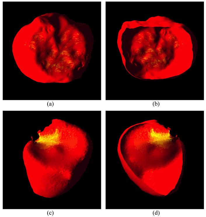
Based on the segmented inner and outer borders, we calculated the thickness of the bladder wall at each voxel position on the inner border. The thickness of bladder wall is expressed as the length of the integral path from a voxel on the inner border to a point on the outer border. If the point is not at the center of a voxel on the outer border, a bi-linear interpolation is needed. The two borders are assumed as two iso-potential surfaces which generate electric potential between them. Therefore, from each point on one surface, one and only one electric field line can be found and traced until termination on the other surface. All electric field lines are smooth and uncrossing. The length of each electric field lines was calculated as the thickness of the bladder wall at the concerned point. Furthermore, the segmentation results were rendered as 3D models with a pseudo-color representing the thickness. From red to yellow, the thickness is increasing. Fig. 17 shows a few examples from the patient datasets. The abnormality is highlighted by yellow patches in Fig. 17(c) and (d).
Fig. 17.
Examples of 3D renderings of a few segmented bladder walls. Picture (a) is an outside view of the segmented outer border of a dataset. Picture (b) is a cut view inside the segmented inner border of the dataset. Picture (c) shows the outside view of the segmented outer border of another dataset. The highlighted yellow patch indicates the area of abnormality. Picture (d) shows the cut view of the segmented inner border of the same dataset with abnormality. The abnormality can be highlighted in the 3D reconstructed bladder because of the thickness variation.
V. DISCUSSION AND CONCLUSION
A coupled level set (LS) framework has been presented for segmentation of the bladder wall using T1-weighted MR images. Each border of the wall is described by a LS function, respectively. The region of interest (ROI) between the borders is described by a regional adaptive clustering algorithm (RACA). The evolution of the LS functions for both the inner and outer borders and the classification of the ROI by the RACA are interleaved together to update the estimates for an optimal segmentation of the bladder wall. Satisfactory results were obtained from both volunteer and patient studies.
Although it suppresses the urine intensity for an excellent image contrast against the bladder wall while mitigating the partial volume (PV) effect, T1-weighted MR imaging suffers several drawbacks as T2-weighted MR imaging, such as intensity inhomogeneity, image artifacts due to urine, bladder and respiration motions, chemical shift and susceptibility effects, and noise. It is impossible to use a theoretical model to describe and mitigate all these disturbances. Therefore, instead of relying on a theoretical model, we turn to focus on the local intensity contrast and prior geometry knowledge. Because of the good contrast between the bladder lumen/urine and wall, the inner border is segmented first by the use of the intensity contrast information. In segmenting the outer border where the contrast on the surrounding soft tissues varies noticeably, the geometric information of the inner border is used. This is based on the knowledge that the early stage abnormality only affects the shape of the inner border and the outer border would have a similar shape as the inner border. (At later stage of tumor growth, the abnormality on the inner border can be detected efficiently and the outer border may not be needed). This makes it possible to initialize the outer LS function (OLSF) close to the outer border. Beside the geometry constraint, the RACA is used to utilize both the global and local intensity contrast to assist the OLSF evolution and, therefore, to mitigate the challenge of segmenting the outer border. While the RACA has some unique properties to describe the ROI between the inner and outer borders of the bladder wall, an alternative approach would be the expectation-maximization (EM) algorithm [30], which has several very nice statistical properties in estimating the model parameters (e.g., the mean and standard deviation in section III.D.3.1). Although the Gaussian statistical model may be acceptable [31], the binary labels for the description of the ROI may not be sufficient in the RACA. A more sophisticated algorithm for the description of the ROI would be a Gaussian statistical model on tissue mixtures to consider the PV effect [32], rather than two discrete labels. This is a research topic under progress.
By the patient studies, we observed in most cases that there was not sufficient image contrast between the outer border and its surrounding tissues. This is a major challenge in addition to those drawbacks above. Improvement on the segmentation of the outer border relies on (i) advancement of MR imaging technologies to enhance the image quality (including enhancing the image contrast of the surrounding tissues of the outer border) and (ii) use of more prior knowledge and geometry information as we did in step 4 of section III. Optimizing the T1 imaging sequence to enhance the image contrast is another topic and is currently under progress.
Another challenge would be the automation of the initialization of the inner LS function (ILSF) for the inner border, because of the significant variation of bladder shape and size in clinic. The active shape model in [33] can be a choice to achieve the automating goal. An alternative would be the use of initial segmentation from a threshold-based method, which may provide a few land markers (e.g., locations of the bone) to locate the initial ZLSF of the ILSF at the center of the bladder. This is another research topic under investigation.
The sample size of patient studies is rather small in this work. Effort has been devoting to recruit more subjects for a larger database to evaluate the presented segmentation method.
ACKNOWLEDGMENTS
This work was supported in part by NIH Grant #CA120917 and #CA082402 of the National Cancer Institute. Dr. Lu was supported by the National Nature Science Foundation of China under grant No.60772020. The authors would appreciate the assistance of Drs. Chris Lee, MD, and Mark Wagshul, PhD, on data acquisition, Drs. Yi Fan, PhD, Lili Zhou, PhD, Bin Liu, PhD, and Zixiao Li, MD, for data processing, and Ms. Aimee Minton for editing this paper.
REFERENCES
- 1.Jemal A, Thomas A, Murray T, Thun M. Cancer statistics. A Cancer Journal for Clinicians. 2002;52:23–47. doi: 10.3322/canjclin.52.1.23. [DOI] [PubMed] [Google Scholar]
- 2.Shaw ST, Poon SY, Wong ET. Routine urinalysis: is the dipstick enough? The Journal of the American Medical Association. 1985;253:1596–1600. doi: 10.1001/jama.253.11.1596. [DOI] [PubMed] [Google Scholar]
- 3.Lamm DL, Torti FM. Bladder cancer. A Cancer Journal for Clinicians. 1996;46:93–112. doi: 10.3322/canjclin.46.2.93. [DOI] [PubMed] [Google Scholar]
- 4.Vining DJ, Zagoria RJ, Liu K, Stelts D. CT cystoscopy: an innovation in bladder imaging. American Journal of Roentgenology. 1996;166:409–410. doi: 10.2214/ajr.166.2.8553956. [DOI] [PubMed] [Google Scholar]
- 5.Hussain S, Loeffler JA, Babayan RK, Fenlon HM. Thin-section helical computer tomography of the bladder: initial clinical experience with virtual reality imaging. Urology. 1997;50(5):685–689. doi: 10.1016/S0090-4295(97)00483-4. [DOI] [PubMed] [Google Scholar]
- 6.Fenlon HM, Bell TV, Ahari HK, Hussain S. Virtual cystoscopy: early clinical experience. Radiology. 1997;205(1):272–275. doi: 10.1148/radiology.205.1.9314998. [DOI] [PubMed] [Google Scholar]
- 7.Merkle M, Wunderlich A, Aschoff AJ, Rilinger N, Gorich J, Bachor R, Gottfried HW, Sokiranski R, Fleiter TR, Brambs HJ. Virtual cystoscopy based on helical CT scan datasets: perspectives and limitations. The British Journal of Radiology. 1998;71:262–267. doi: 10.1259/bjr.71.843.9616234. [DOI] [PubMed] [Google Scholar]
- 8.Song JH, Francis IR, Platt JF, Cohan RH, Mohsin J, Kielb SJ, Korobkin M, Montie JE. Bladder tumor detection at virtual cystoscopy. Radiology. 2001;218:95–100. doi: 10.1148/radiology.218.1.r01ja4995. [DOI] [PubMed] [Google Scholar]
- 9.Kim JK, Ahn JH, Park T, Ahn HJ, Kim CS, Cho K-S. Virtual cystoscopy of the contrast material-filled bladder in patients with gross hematuria. American Journal of Roentgenology. 2002;179:763–768. doi: 10.2214/ajr.179.3.1790763. [DOI] [PubMed] [Google Scholar]
- 10.Rousson M, Khamene A, Diallo M, Celi JC, Sauer F. Constrained surface evolutions for prostate and bladder segmentation in CT images. Lecture Notes in Computer Science. 2005;3765:251–260. [Google Scholar]
- 11.Jaume S, Ferrant M, Macq B, Hoyte L, Fielding JR, Schreyer A, Kikinis R, Warfield SK. Tumor detection in the bladder wall with a measurement of abnormal thickness in CT scans. IEEE Transactions on Biomedical Engineering. 2003;50(3):383–390. doi: 10.1109/TBME.2003.808828. [DOI] [PubMed] [Google Scholar]
- 12.Fielding JR, Hoyte L, Okon SA, Schreyer A, Lee J, Zou KH, Warfield S, Richie JP, Loughlin KR, O’Leary MP, Doyle CJ, Kikinis R. Tumor detection by virtual cystoscopy with color mapping of bladder wall thickness. The Journal of Urology. 2002;167:559–562. doi: 10.1016/S0022-5347(01)69085-2. [DOI] [PubMed] [Google Scholar]
- 13.Liang Z, Chen D, Button T, Li H, Huang W. Feasibility studies on extracting bladder wall from MR images for virtual cystoscopy. Proc. International Society of Magnetic Resonance in Medicine. 1999;3:2204. [Google Scholar]
- 14.Chen D, Li B, Huang W, Liang Z. A multi-scan MRI-based virtual cystoscopy. Proc. SPIE Medical Imaging. 2000;3978:146–152. [Google Scholar]
- 15.Bernhardt TM, Rapp-Bernhardt U. Virtual cystoscopy of the bladder based on CT and MRI data. Abdominal Imaging. 2001;26:325–332. doi: 10.1007/s002610000168. [DOI] [PubMed] [Google Scholar]
- 16.Bernhardt TM, Schmidl H, Philipp C, Allhoff EP, Rapp-Bernhardt U. Diagnostic potential of virtual cystoscopy of the bladder: MRI vs CT. preliminary report. European Radiology. 2003;13:305–312. doi: 10.1007/s00330-002-1444-9. [DOI] [PubMed] [Google Scholar]
- 17.Lämmle M, Beer A, Settles M, Hannig C, Schwaibold H, Drews C. Reliability of MR imaging-based virtual cystoscopy in the diagnosis of cancer of the urinary bladder. American Journal of Roentgenology. 2002;178:1483–1488. doi: 10.2214/ajr.178.6.1781483. [DOI] [PubMed] [Google Scholar]
- 18.Li L, Wang Z, Harrington D, Huang W, Liang Z. A mixture-based computed aided detection system for virtual cystoscopy. Proc. International Society of Magnetic Resonance in Medicine. 2003;1:146. [Google Scholar]
- 19.Li L, Wang Z, Li X, Wei X, Adler H, Huang W, Rizvi S, Meng H, Harrington D, Liang Z. A new partial volume segmentation approach to extract bladder wall for computer aided detection in virtual cystoscopy. Proc. SPIE Medical Imaging. 2004;5369:199–206. [Google Scholar]
- 20.Li L, Liang Z, Wang S, Lu H, Wagshul M, Zawin M, Posniak E, Lee C. Segmentation of multi-spectral bladder MR images with inhomogeneity correction for virtual cystoscopy. Proc. SPIE Medical Imaging, in CD-ROM. 2008 [Google Scholar]
- 21.Osher S, Sethian J. Fronts propagating with curvature dependent speed: algorithms based on Hamilton-Jacobi formulation. Journal of Computer Physics. 1988;79:12–49. [Google Scholar]
- 22.Costa MJ, Delingette H, Novellas S, Ayache N. Automatic segmentation of bladder and prostate using coupled 3D deformable models. Proceedings of MICCAI. 2007:252–260. doi: 10.1007/978-3-540-75757-3_31. [DOI] [PubMed] [Google Scholar]
- 23.Sethian JA. Level Set Methods and Fast Marching Methods: Evolving interfaces in computational geometry, fluid mechanics, computer vision, and materials science. 2nd ed. Cambridge University Press; 1999. [Google Scholar]
- 24.Chan T, Vese L. Active contours without edges. IEEE Transactions on Image Processing. 2001;10(2):266–277. doi: 10.1109/83.902291. [DOI] [PubMed] [Google Scholar]
- 25.Vese LA, Chan TF. A multiphase level set framework for image segmentation using the Mumford and Shah model. International Journal of Computer Vision. 2002;50(3):271–293. [Google Scholar]
- 26.Pappas TN. An adaptive clustering algorithm for image segmentation. IEEE Transactions on Signal Processing. 1992;40(4):901–914. [Google Scholar]
- 27.Derin H. Proceedings of CISS-86. 1986. Experimentations with simulated annealing in allocation optimization problems; pp. 165–171. [Google Scholar]
- 28.Chambers JM, Hastie TJ. Statistical Models. S. Wadsworth & Brooks/Cole; 1992. [Google Scholar]
- 29.Pinheiro JC, Bates DM. Mixed-Effects Models in S and S-PLUS. New York: Springer; 2000. [Google Scholar]
- 30.Dempster A, Laird N, Rubin D. Maximum likelihood from incomplete data via the EM algorithm. Journal of the Royal Statistical Society (JRSS) 1977;39B:1–38. [Google Scholar]
- 31.Chen Y-T, Tseng D-C. Medical image segmentation based on the Bayesian level set method. Lecture Notes in Computer Science - Medical Imaging and Informatics. 2008;4987:25–34. [Google Scholar]
- 32.Liang Z, Wang S. An EM approach to MAP solution of segmenting tissue mixtures: a numerical analysis. IEEE Transactions on Medical Imaging. 2009;28(2):297–310. doi: 10.1109/TMI.2008.2004670. [DOI] [PMC free article] [PubMed] [Google Scholar]
- 33.Cootes TF, Taylor CJ, Cooper DH, Graham J. Active shape models – their training and application. Computer Vision and Image Understanding. 1995;61(1):38–59. [Google Scholar]


