

Abstract
Dynamic contrast-enhanced magnetic resonance imaging (DCE-MRI) is a widely used technique for assessing tissue physiology. Spoiled gradient echo (SPGR) pulse sequences are one of the most common methods for acquisition of DCE-MRI data, providing high temporal and spatial resolution with strong T1-weighting. Conversion of SPGR signal to concentration is briefly reviewed, and a new closed-form expression for concentration measurement uncertainty for finite signal-to-noise ratio (SNR) and baseline scan time is derived. This result is applicable to arbitrary concentration-dependent relaxation rate and is valid over the same domain as the theoretical SPGR signal equation. Expressions for the lower and upper bounds on measurable concentration are also derived. The existence of a concentration- and tissue-dependent optimal flip angle that minimizes concentration uncertainty is demonstrated and it is shown that, for clinically relevant pulse sequence parameters, this optimal flip angle is significantly larger than the corresponding Ernst angle. Analysis of three pulse sequences from the DCE-MRI literature shows that optimization of flip angle using the methods discussed here leads to potential improvements of 10-1166% in effective SNR over the 0.5-5.0 mM concentration range with minimal or no loss of measurement accuracy down to 0.1 mM. In vivo data from three study patients provide further support for our theoretical expression for concentration measurement uncertainty, with predicted and experimental estimates agreeing to within ±30%. Equations for concentration bias resulting from biases in flip angle and from pre-contrast relaxation time and contrast relaxivity (both longitudinal and transverse) are also derived in closed-form. The resulting equations show the potential for significant contributions to bias in concentration measurement arising from even relatively small mis-specification of flip angle and/or pre-contrast longitudinal relaxation time, particularly at high contrast concentrations.
1. Introduction
Pharmacokinetic (PK) modeling of dynamic contrast-enhanced magnetic resonance imaging (DCE-MRI) data has emerged as a standard method for gaining insight into tissue physiology in cancer imaging, cardiac and cerebral perfusion, inflammatory disorders and a number of other areas (Collins and Padhani 2004, Jackson et al 2003, Leach et al 2003). Reproducible calculation of PK model parameters depends on the ability to reliably and consistently determine quantitative contrast concentrations in both the blood and tissue from the measured MRI signal. Spoiled gradient echo (SPGR) pulse sequences are one of the most commonly used methods of DCE-MRI data collection, enabling rapid acquisition of highly T1-weighted images with good spatial coverage and resolution. Here we briefly review the conversion of SPGR signal measurements to contrast concentration using the SPGR signal equation. We then derive a new closed-form expression for concentration measurement uncertainty as it depends on the signal-to-noise ratio (SNR) and number of pre-contrast baseline scans (NB). Novel expressions for minimum detectable concentration, Cdet, and saturation concentration, Cmax, are derived, as well as expressions for concentration biases resulting from mis-specification of flip angle (α), pre-contrast longitudinal and transverse relaxation time (T1,0 and , respectively), and longitudinal and transverse contrast relaxivities (r1 and , respectively). The existence of a concentration- and tissue-dependent optimum flip angle for which the measurement uncertainty is minimized and that differs substantially from the Ernst angle over the clinically relevant contrast concentration range for a wide range of pulse sequence parameters is also shown.
We demonstrate the utility of the uncertainty expressions derived here by considering three pulse sequences reported in the recent DCE-MRI literature and investigating the potential improvement in effective SNR achievable by flip angle optimization in the concentration range normally observed for tissues in vivo. Concentration biases resulting from uncertainty in measurement of flip angle and pre-contrast longitudinal relaxation time on AIF and tissue curves are estimated and plotted, showing that the choice of pulse sequence parameters also has a large impact on sensitivity to uncertainty in these parameters. Finally, our theoretical calculations for concentration measurement uncertainty are compared with in vivo measurements of the AIF and tissue curves in tumors in humans, demonstrating that it is possible to predict these uncertainties with reasonable accuracy a priori from SNR and image acquisition parameters. These results complement investigations of the precision with which PK model parameters can be estimated (Buckley 2002, Dale et al 2003, Kershaw and Buckley 2006, Schmid et al 2005) by providing a means of accurately computing the uncertainty in the concentration measurements that are subsequently input into regression models.
2. Theory
2.1. Relative signal enhancement with contrast concentration
In DCE-MRI, the observed temporal signal stems entirely from time-varying longitudinal (T1) and transverse effective relaxation times that, in turn, only depend on contrast agent concentration, C = C(t). The basic theoretical expression for spoiled gradient echo signal intensity (S) at steady state is (Bernstein et al 2004)
| (1) |
where M0 is the signal for α = 90° in the limit TR, TE → 0, and includes both proton density and system gain contributions. The relative signal enhancement is defined as
| (2) |
where T1,0 and are the pre-contrast longitudinal and transverse effective relaxation times, respectively. The following discussion is simplified by the use of relaxation rates rather than relaxation times. The pre-contrast longitudinal and transverse relaxation rates are defined as the inverses of the corresponding relaxation times: R1,0 = 1/T1,0 and , respectively. The specific functional forms of the concentration dependent relaxation rates, R1 = R1(C) and , depend on details of the underlying mechanisms of contrast enhancement (Landis et al 1999, Yankeelov et al 2003, Conturo et al 2005). In the fast exchange limit (FXL) commonly used for analysis of DCE-MRI data, these relaxation rates scale linearly with contrast concentration:
| (3a) |
| (3b) |
To further simplify our equations, we define E1,0 = exp(-TR R1,0), E1 = exp(-TR R1), and in terms of the pre- and post-contrast longitudinal and transverse relaxation rates. Using these definitions, equation (2) becomes
| (4) |
The dependence on the spatially dependent system gain function has been eliminated in the expression for relative enhancement given in equation (4), making this method insensitive to coil receive inhomogeneity, unlike methods looking at signal differences alone. In addition, in the FXL this method is insensitive to variation in the pre-contrast transverse relaxation time, . While these properties are desirable, it should be noted that this approach requires a relatively low-noise pre-contrast baseline measurement. Alternative approaches exist, including direct use of the measured signal, where M0 and/or are estimated or modeled. While we do not specifically address those approaches here, the error analysis should be largely similar to that described in the following with the exception of added error terms for M0 and .
The concentration dependence of Ξ from equation (2) is plotted for several different sets of imaging parameters and tissue types in figure 2 (more details are provided in the results section). Clearly, in the low concentration limit, Ξ → 0 as . Similarly, in the high concentration limit, Ξ → -1 as . Between these two extremes, there is a concentration value, Cmax, at which Ξ reachecs a maximum value, Ξmax. We denote the solution of equation (4) for concentration as a function of relative signal enhancement by C(Ξ), where the concentration dependence is contained in the E1 and E2 terms. It has no positive real solutions for Ξ < -1 or Ξ > Ξmax since Ξ is bounded by -1 ≤ Ξ ≤ Ξmax. It is two-valued for 0 ≤ Ξ < Ξmax because there is one solution below Cmax and a second above it, and is single-valued in the high concentration regime where -1 ≤ Ξ < 0. There does not appear to be a general closed-form solution of equation (4) forC(Ξ), but this equation can be solved numerically to determine the concentration of contrast for any measured value of Ξ assuming attention is paid to the selection of the appropriate one of the two possible solutions. Furthermore, if we make the common simplifying assumption that relaxation can be neglected, we obtain a single-valued expression:
| (5) |
Unlike equation (4), equation (5) can easily be solved for R1 to obtain a nonlinear analytic approximation:
| (6) |
To this point we have made no assumptions about the details of the concentration dependence of the relaxation rates. Using the fast exchange limit from equation (3a), we can obtain a closed-form approximation for C in terms of the solution of R1 from equation (6):
| (7) |
Equation (7) is equivalent to equation (7) of (Dale et al 2003) and equation (5) of (Heilmann et al 2006). In the low concentration limit, we can expand equation (4) to linear order in C and take the limTR, TE→0 to obtain the commonly used linear approximation (Tofts 1997, Workie et al 2004):
| (8) |
While these approximations provide a convenient means of converting signal to concentration, use of either equation (7) or equation (8) can result in significant, systematic underestimation of C even at fairly modest contrast concentrations. Equation (8) is particularly poor in many circumstances. For this reason, a numerical solution of equation (4) should generally be preferred over approximate expressions for quantitative DCE-MRI applications unless it is certain that the concentrations to be measured will remain within the range of validity of those approximations.
Figure 2.

Concentration dependence of Ξ from equation (4) for three sets of pulse sequence parameters: PS1 (panels (a), (b)), PS2 (panels (c), (d)) and PS3 (panels (e), (f)). Curves are plotted for three different tissue types: arterial blood (solid red lines), skeletal muscle (dashed green lines) and liver tissue (dotted purple lines). The panels in the first column are plotted on a logarithmic concentration scale to show the overall behavior of Ξ more clearly over a broad range, while the panels in the second column are plotted on a linear scale spanning the approximate range of clinical interest.
2.2. Uncertainty and sensitivity analysis
In the following, we develop a closed-form solution for concentration measurement uncertainty stemming from uncertainty in the measured relative signal enhancement (Ξ) that incorporates the effects of finite signal-to-noise ratio and number of pre-contrast baseline measurements. We also present solutions for the sensitivity of concentration measurement to uncertainty in the specification of flip angle (α), pre-contrast longitudinal (T1,0) and transverse relaxation times, and longitudinal (r1) and transverse contrast relaxivities.
2.2.1. Ξuncertainty
Considering concentration to be a (multi-valued) function of Ξ, C = C(Ξ), and neglecting covariance between parameters, we use the standard theory of propagation of errors to determine the variance in C corresponding to a variance in measurement of Ξ:
| (9) |
In general, the neglect of covariance should be a good approximation as there is no a priori reason to expect correlated noise between the measured signal and measured flip angle, relaxation times, or relaxivities as the latter parameters will generally be measured using separate pulse sequences. The partial derivative ∂C/∂Ξ, representing the sensitivity of concentration to signal enhancement, is computed by implicitly differentiating equation (4) with respect to Ξ to obtain
| (10) |
where
| (11) |
Equation (11) is valid when equation (1) and the relaxation rate formalism are both valid. In particular, it can be used even when the relationship between concentration and relaxation rate is nonlinear (Conturo et al 2005, Landis et al 1999). In the fast exchange limit of equation (3), this expression reduces to
| (12) |
Using the definition of Ξ from equation (2), and defining the pre- and post-contrast signals as and respectively, we obtain the variance in Ξ:
| (13) |
In a typical DCE-MRI experiment, NB independent pre-contrast baseline measurements are averaged together to determine S0. These pre-contrast measurements are followed by a series of one or more post-contrast measurements, each of which is independent. We denote the noise variance of a single voxel measurement, neglecting systematic physiological noise contributions (motion, flow, etc), as var(S). That is, var(S) is the variance in measured signal that would be obtained from a sequence of repeated measurements of a single voxel of a static object with unchanging acquisition parameters. Assuming that the coil configuration and receiver bandwidth do not change and the proton density, conductivity and temperature of the object being imaged remain constant throughout the measurement, it is well established that this noise variance does not depend on pulse sequence parameters used for data acquisition (e.g. TR/TE/α), although it does depend on the total number of measurements (acquisition time) in the usual way (Parker and Gullberg 1990, Kruger and Glover 2001). In particular, the injection of contrast has no effect on the noise variance despite the resulting increase in signal for heavily T1-weighted pulse sequences. Because each individual dynamic measurement is independent of the others, the noise variance in the average of the precontrast measurements, S0, is simply given by var(S0) = var(S)/NB. With this we can simplify the previous expression to obtain
| (14) |
Setting the noise variance to be var(S) = (S0/SNR)2 (with SNR defined as the ratio of the mean measured pre-contrast signal to its standard deviation) and substituting equations (1), (10), and (14) into equation (9), we obtain a final expression for the variance in concentration measurement,
| (15) |
which is applicable over the entire domain for which the signal equation itself is valid.
The absolute and relative uncertainties in C can now be defined as
| (16a) |
| (16b) |
As expected, both ∊abs and ∊rel are inversely proportional to the SNR (or, equivalently, proportional to noise), vanish uniformly in the limit SNR → ∞, and diverge in the limit NB → 0. The change in the effective SNR value that is obtained by increasing the number of baseline measurements from NB,1 to NB,2 is given by (using the inverse equivalence of uncertainty and SNR)
| (17) |
with the following limiting values:
| (18a) |
| (18b) |
| (18c) |
The maximum value of f is attained when S is maximized, as can be readily demonstrated by differentiation of equation (17).
2.2.2. Detection envelope
Equation (15) can be used to derive an approximate expression for the concentration detection threshold, Cdet, by computing the absolute uncertainty in the low concentration limit:
| (19) |
where β’ is obtained by taking the limC → 0 β (equivalent to limE1 → E1,0) in equation (11). This equation is valid as long as the concentration dependence of ∊abs is weak for C ≈ Cdet. For small TR and TE, this can be further simplified to
| (20) |
The fact that the detection threshold is inversely proportional to the SNR means that Cdet can be made arbitrarily small by increasing the signal-to-noise ratio, up to the point where other unmodeled sources of error dominate.
We can derive a complementary expression for the saturation (maximum measurable) concentration, Cmax, by solving ∂Ξ/∂C = 0. For the general case, the solution must be expressed in terms of the longitudinal relaxation time, which can then be solved for concentration (either analytically or numerically):
| (21) |
where
| (22a) |
| (22b) |
In the fast exchange limit, we can solve for concentration directly:
| (23) |
The corresponding maximum value of [Ξ] can be obtained by direct back-substitution of Cmax into equation (4). For flip angles less than
| (24) |
Cmax becomes negative, so there will be no signal enhancement for 0 ≤ α ≤ αmin with contrast administration.
2.2.3. α sensitivity
The flip angle can vary significantly from its nominal value, particularly at high field or when local RF transmit coils are used (Treier et al 2007). Thus, it is of interest to assess the effect of biases in estimates of α on the corresponding estimates of C. Implicitly differentiating equation (4) with respect to α, we obtain an expression for the concentration sensitivity to flip angle variation:
| (25) |
We can then write the relative bias in concentration measurement stemming from a bias in flip angle of δα as
| (26) |
Assuming that the FXL holds, this bias approaches
| (27) |
in the low concentration limit, going to zero in the limit TR ≪ T1,0
2.2.4. T1,0 sensitivity
Longitudinal relaxation time is known with limited precision due to measurement error, partial volume effects, heterogeneity of the local chemical environment, flow effects, etc. Proceeding as in the previous section, T1,0 concentration sensitivity is
| (28) |
with relative concentration bias for a T1,0 bias of δT1,0 given by
| (29) |
In the fast exchange limit at low concentration and for short echo time, the bias becomes
| (30) |
If repetition time is also small, this becomes a negative concentration bias proportional to relative pre-contrast relaxation time bias:
| (31) |
2.2.5. sensitivity
Proceeding as in the previous section, the concentration sensitivity to uncertainty in pre-contrast transverse effective relaxation time, , is
| (32) |
In the fast exchange limit, the partial derivative of with respect to becomes (from differentiation of equation (3b)), so the bias vanishes, demonstrating that measurement of concentration is independent of in this limit.
2.2.6. r1 and sensitivity
In general, contrast relaxivity is determined from in vitro measurements of the concentration dependence of relaxation time. Such measurements may fail to account for the observed variation of relaxivity with macromolecular content. The precise magnitude of this effect is difficult to quantify in vivo, although (Stanisz and Henkelman 2000) report that typical macromolecular content in the interstitial fluid could lead to in vivo r1 values being 30-70% greater than those measured in vitro. The r1 concentration sensitivity is
| (33) |
which gives, in the fast exchange limit, a negative relative concentration bias proportional to the relative r1 bias,
| (34) |
at low concentrations.
Similarly, concentration sensitivity is
| (35) |
giving a relative concentration bias in the fast exchange limit of
| (36) |
at high concentrations where transverse relaxation effects become dominant.
3. Methods
3.1. In vitro measurements
In order to test the accuracy of the theoretical SPGR signal equation for modeling measurement data, we performed in vitro experiments with a phantom spanning the concentration range from C = 0-100 mM. Measurements were performed on a 3 T Siemens Trio system using the body coil for transmit to minimize flip angle inhomogeneity. The phantom consisted of a set of 30 glass vials approximately 1 cm in diameter and 5 cm in length, filled with mixtures of saline solution and various amounts of gadodiamide (Omniscan) and sealed with airtight caps to exclude air bubbles. Vials were oriented in the magnet bore parallel to the main field axis to eliminate susceptibility-induced image distortion at the air-fluid interface. Concentrations were 0.0000, 0.0344, 0.0536, 0.0680, 0.0946, 0.210, 0.260, 0.359, 0.508, 0.607, 0.693, 0.946, 1.26, 1.65, 2.04, 2.58, 3.22, 4.09, 5.20, 6.42, 8.30, 13.6, 14.5, 19.3, 30.7, 42.3, 51.2, 65.0, 79.6 and 102 mM. Longitudinal relaxation time was measured using a single slice real inversion recovery turbo spin echo (IRSE) sequence with TR = 5000 ms, TE = 15 ms and a turbo factor of 9. An imaging matrix of 192 × 96 with a field of view (FOV) of 115 mm × 58 mm resulted in a spatial resolution of 0.6 ×0.6 mm, with slice thickness set at 8 mm. Inversion times of TI = 22, 25, 30, 35, 40, 50, 100, 200, 300, 400, 500, 600, 800 and 1600 ms were measured. T1 for each vial was determined by nonlinear regression to the signal equation for a real IRSE sequence:
| (37) |
where k is equal to the cosine of the flip angle of the inversion pulse. Linear regression to curves of 1/T1 versus C gave a longitudinal relaxivity of the gadodiamide contrast of r1 = 3.4 mM-1 s-1. T2 relaxation time was determined using a single slice multi-echo spin echo sequence with 32 echoes evenly spaced between 14.3 and 457.6 ms, inclusive, giving a transverse relaxivity of r2 = 4.4 mM-1 s-1 from linear regression to curves of 1/T2 versus C. These values of relaxivity are in good agreement with values reported in the literature at 3 T (Rohrer et al 2005). A three-dimensional spoiled gradient echo sequence was used for the simulated ‘dynamic’ measurements, with TR = 8.8 ms, TE = 1.31 ms, and sixteen 5 mm slices centered on the vial. Images were acquired for seven flip angles ranging from 10° to 40° in 5° increments. Each scan was averaged ten times to reduce noise. A single central slice (slice 8) was analyzed to minimize the effects of flip angle variation near the slab boundaries. Regions of interest were chosen to avoid partial-volume effects near the vial-air interface.
3.2. In vivo measurements
To test our theoretical uncertainty predictions with in vivo data, we measured arterial input functions and tissue concentration curves in three patients from whom informed consent was obtained under an IRB-approved protocol. Measurements were made using a three-dimensional spoiled gradient echo sequence (fl3d) on a 1.5 T Siemens TIM Avanto scanner. Pulse sequence parameters for these three data sets are given in table 1. Patient 1 was scanned near the distal humerus, with AIF measured in the brachial artery and the tissue curve in a neurofibroma. Patient 2 was scanned across the pelvis and proximal femur, with AIF measured in the iliac and femoral arteries and the tissue curve in a Ewing’s sarcoma. Patient 3 was scanned in proximity to the acromio-clavicular joint, with AIF measured in the brachial artery and the tissue curve in a metastatic primitive neuroectodermal tumor. The number of slices ranged from 16 to 36, with dynamic acquisitions lasting from 6 to 9 min, including ten frames of baseline scanning prior to contrast injection. The body coil was used for RF transmission to maximize RF homogeneity. Flip angle variation along the slab encoding direction was estimated using a homogeneous phantom of known T1,0, and, in the three study patients, by assuming a constant T1,0 value of 240 ms for subcutaneous fat. These experiments indicated that the impact of flip angle variation near the slab boundaries was small except for roughly the outer 10% of slices at each boundary, so these slices were excluded from the analysis. 20 ml (∼ 0.1-0.2 mmol kg-1) of gadolinium contrast agent (Omniscan) was injected into the antecubital vein through a 20 ga IV at a constant rate of 4 ml s-1 followed by a 20 ml saline flush at 2 ml s-1 using a Medrad Spectra Solaris power injector. Contrast injection was timed to coincide with the end of acquisition of the 10th frame of dynamic data. Pre-contrast signal intensity, S0, was determined by averaging the baseline data acquired prior to injection and SNR from the ratio of the baseline signal to its standard deviation. T1,0 and of arterial blood were taken to be 1440 and 290 ms, respectively (Stanisz et al 2005). Tissue T1,0 values were estimated using a variable flip angle method with flip angles of 5°/10°/20°/30° (Fram et al 1987). In vivo Gd relaxivities at 1.5 T of r1 = 4.3 mM-1 s-1 and and the fast exchange limit were assumed (Rohrer et al 2005).
Table 1.
Pulse sequence parameters for in vivo data acquisition. Δt represents the sampling time per frame
| TR | TE | α | Δ t | Resolution (mm) | SNR | NB | |
|---|---|---|---|---|---|---|---|
| Patient 1 | 3.31 ms | 1.27 ms | 20° | 5.59 | 1.25 × 1.25 × 2 | 5.3 | 10 |
| Patient 2 | 2.81 ms | 1.29 ms | 20° | 4.72 | 0.94 × 0.94 × 6 | 7.9 | 10 |
| Patient 3 | 3.80 ms | 1.40 ms | 20° | 4.94 | 0.94 × 0.94 × 3 | 6.5 | 10 |
Partial volume effects can lead to systematic underestimation of peak plasma concentration (van Osch et al 2005, Rijpkema et al 2001). These were minimized by using an interactive, semi-automated procedure to identify AIF voxels. Initially, coarse regions of interest (ROI) were identified where candidate AIF voxels were to be sought. Within this manually selected ROI, we computed the absolute maximum value of Ξ, denoted , which ideally should correspond to the voxel with the greatest peak concentration (and, consequently, the least partial volume contamination). An empirical threshold value (χ) of 75% was chosen and the AIF computed by selecting voxels within the ROI whose maximum relative signal enhancement value, , satisfied . The resulting voxels were then averaged together to generate a time curve of relative enhancement, Ξ(t). Blood inflow effects were minimized by imaging arteries so that they were oriented primarily in-plane and excluding arterial voxels transverse to the imaging planes from the initial manual ROI.
4. Results
4.1. In vitro measurements
The theoretical and measured (in vitro) curves of signal, S, and relative signal enhancement, Ξ, for our concentration phantom are compared in figure 1. Figure 1(a) shows the measured signal for the concentration phantom (black points), along with the result of regressing the signal-concentration curves to the theoretical expression from equation (1) with M0 as a regression parameter and flip angle fixed at the nominal value (solid black line) and with both M0 and α as free parameters (dashed gray line). Clearly, we obtain excellent agreement in both cases, indicating that the theoretical signal equation is sufficiently accurate to describe these data. The mean error in α determined from the latter regressions was 0.13 ± 0.73°. Curves for relative signal enhancement, Ξ, and regressions using equation (4) with α free are shown in figure 1(b), with comparably good agreement. Because the phantom vials were all simultaneously scanned, the different concentrations are measured at spatially varying locations, and any residual spatial variation in flip angle will lead to systematic errors in Ξ. This effect is small in our case, as demonstrated by the relatively small deviation of α from its nominal values, but serves to emphasize the importance of considering the possibility of flip angle variation from the nominal value when making contrast concentration measurements. The spatial variation in α manifests itself primarily in the slight systematic variation, correlated between flip angles, that is visible near the peak in figure 1. Nevertheless, these phantom results clearly demonstrate that the theoretical expressions in equations (1) and (4) can be used to accurately model experimental MRI measurements.
Figure 1.

Experimentally measured signal (panel (a)) and relative signal enhancement (panel (b)) plotted as a function of C in a concentration phantom for flip angles ranging from 10° to 40°. In panel (a), the solid black lines show regression of equation (1) to the measured data with M0 as the only free parameter, while the dashed gray lines show the result of regression with both M0 and α free. The dashed gray lines in panel (b) are the corresponding regression curves for equation (4).
4.2. Theory
The practical impact of concentration measurement uncertainty is demonstrated by analyzing the error characteristics of SPGR sequences from three recently published DCE-MRI papers that reported pharmacokinetic modeling results in human cancer patients (Pickles et al 2005, Batchelor et al 2007, Yankeelov et al 2007). Imaging parameters for these pulse sequences, denoted PS1 (Pickles et al 2005), PS2 (Batchelor et al 2007) and PS3 (Yankeelov et al 2007), as reported in the original references, are given in table 2. Because signal-to-noise ratios were not provided in any of the cited references, the SNR was chosen to be in the typical range of values for a single voxel measurement in a DCE-MRI experiment at our institution. In order to ensure a fair comparison of these sequences, we assume that the SNR efficiency is constant and equal to (Parker and Gullberg 1990), equivalent to the case where three consecutive scans are performed using PS1, PS2 and PS3 on the same system without changing any other aspect of the data collection. Estimated values of the actual SNR in the three cited studies (computed by assuming coil performance comparable to that of our system and scaling by the ratio of the products) are substantially higher due to the larger voxels used: 14-32 for PS1, 23 for PS2 and 38 for PS3. For this reason, the error figures derived here are only demonstrative and do not directly apply to the results reported in the original papers. We consider three different tissue types chosen to span the range of T1,0 values typically seen in vivo: arterial blood (solid red lines), skeletal muscle (dashed green lines) and liver tissue (dotted purple lines). Reference values for the relaxation times of these tissues are given in table 3. Longitudinal and transverse relaxivities were set to the values used in our in vivo analysis: r1 = 4.3 mM-l S-1 and .
Table 2.
Pulse sequence parameters for simulated SPGR data. Values for PS1 were taken from (Pickles et al 2005), for PS2 from (Batchelor et al 2007) and for PS3 from (Yankeelov et al 2007)
| TR (ms) | TE (ms) | α | Δt (s) | Resolution (mm) | SNRa | NB | |
|---|---|---|---|---|---|---|---|
| PS1 | 7.6 | 4.20 | 30° | 11.6 | 0.8 × 1.6 × 4-9 | 5.0 | 3b |
| PS2 | 5.7 | 2.73 | 10° | 5.04 | 2.9 × 2.0 × 2.1 | 4.3 | 10c |
| PS3 | 200 | 1.80 | 30° | 52 | 0.8 × 1.6 × 5 | 25.6 | 2d |
The referenced papers do not provide estimates of SNR, so a value of 5 was chosen for PS1 and the values for PS2 and PS3 computed assuming constant SNR efficiency.
NB was not reported, but appears to be in the range of 2-3 from the figures in the cited paper.
NB was reported to be 10.
NB was not reported, but appears to be 2 from the figures in the cited paper.
Table 3.
Tissue parameters at 1.5 T for simulated SPGR data (from (Stanisz et al 2005))
| T1,0 | ||
|---|---|---|
| Arterial blood | 1441 ms | 290 ms |
| Skeletal muscle | 1008 ms | 44 ms |
| Liver tissue | 576 ms | 46 ms |
Curves of Ξ (C) for the three pulse sequences are plotted in figure 2, with PS1 in the top row, PS2 in the middle and PS3 in the bottom. The left-hand panels ((a), (c), (e)) are shown over a logarithmic concentration scale ranging from 10-3 to 103 mM to demonstrate the overall shape including the peak at Cmax and subsequent decrease to a limiting value of limC → ∞ Ξ = -1. The same curves are plotted on a linear scale over the approximate range of clinically relevant concentrations (0-10 mM) in the right-hand panels ((b), (d), (f)). Figure 3 shows the flip angle dependence of Cmax for PS1-PS3. Cmax shows minimal dependence on T1,0 for all three pulse sequences, with the greatest deviation seen for PS3 for liver tissue. Increasing α continuously increases the maximum concentration that may be measured without saturation up to α = 180°. However, the decrease in total signal as flip angle exceeds the Ernst angle ultimately limits the ability to measure large concentrations by increasing flip angle. Furthermore, SAR exposure increases with increasing flip angle, which will also constrain achievable flip angle values. Values for Cdet from equation (19), Cmax from equation (23), Ξmax, and Ernst angle (αE = cos-1 E1,0) for the various pulse sequences and tissues are given in table 4.
Figure 3.

Flip angle dependence of the saturation concentration, Cmax, from equation (23) for PS1 (panel (a)), PS2 (panel (b)) and PS3 (panel (c)). Tissue types are shown as in figure 2.
Table 4.
Concentration detection threshold (Cdet), saturation concentration (Cmax), maximum relative signal enhancement (Ξmax), and Ernst angle (αE) for the three pulse sequences and three tissue types used in our simulations
| Cdet | Cmax | Ξ max | α E | ||
|---|---|---|---|---|---|
| Arterial blood | PS1 | 0.039 mM | 11.88 mM | 14.90 | 5.9° |
| PS2 | 0.050 mM | 6.16 mM | 3.06 | 5.1° | |
| PS3 | 0.015 mM | 2.92 mM | 0.83 | 29.5° | |
| Skeletal muscle | PS1 | 0.056 mM | 11.81 mM | 10.31 | 7.0° |
| PS2 | 0.077 mM | 6.09 mM | 2.09 | 6.1° | |
| PS3 | 0.026 mM | 2.85 mM | 0.55 | 34.9° | |
| Liver tissue | PS1 | 0.103 mM | 11.64 mM | 5.73 | 9.3° |
| PS2 | 0.164 mM | 5.92 mM | 1.13 | 8.0° | |
| PS3 | 0.068 mM | 2.67 mM | 0.28 | 45.0° |
4.2.1. Relative concentration uncertainty
Figure 4 shows the relative concentration uncertainty, ∊rel, for each of the three pulse sequences and three tissue types. The panels in the left column ((a), (c), (e)) are plotted over the approximate clinical range of interest, 0-10 mM, while those in the right column ((b), (d), (f)) are plotted over a narrower range (0-2 mM) that is typical of tissue enhancement seen in vivo. Clearly, PS1 (panels 4(a) and (b)) is the most accurate of the three sequences, with a relatively broad minimum and only weak dependence of uncertainty on T1,0. In contrast, both PS2 and PS3 have uncertainties that increase much more rapidly with increasing C and exhibit much greater sensitivity to tissue type. The uncertainties of PS2 and PS3 are larger because the nonlinear regime of concentration saturation is near (or within) the clinically interesting concentration range. The observation that increasing α increases saturation concentration suggests that the use of a larger flip angle in these pulse sequences could provide improved measurement accuracy; this is addressed in more detail in the section below on flip angle optimization. The downward sloping curves in the upper right corner of panel 4(e), where relative uncertainty is decreasing with increasing concentration, correspond to the parameter regime dominated by effects where C < Cmax. Because the analysis of signal behavior in the dynamic susceptibility contrast (DSC) regime is complicated by the mesoscale effects of the contrast-induced susceptibility gradients and their interaction with vessel size distribution (Kiselev 2004), we restrict our discussion here to the T1-weighted DCE-MRI regime.
Figure 4.

Relative concentration measurement uncertainty from equation (16b), for PS1 (panels (a), (b)), PS2 (panels (c), (d)), and PS3 (panels (e), (f)) for the three tissue types in figure 2, assuming SNR and NB as given in table 1. The panels in the first column are plotted over the approximate concentration range of clinical interest, while those in the second column are plotted over a smaller range representative of concentrations seen in tissues in vivo.
As demonstrated above, changes in ∊abs and ∊rel are always inversely proportional to changes in SNR, so that doubling the signal-to-noise ratio results in a halving of the concentration uncertainty. The effect of changing the number of background measurements is more complex, but can be regarded as producing a concentration-dependent change in the effective SNR. The change in the SNR (f from equation (17)) obtained by increasing the number of baseline measurements from one to NB is plotted in figure 5 for NB 2, 5, 10 and 20. The limiting values given by equation (18b) and equation (18c) are indicated by the lower and upper horizontal lines, respectively. From the figure, it is apparent that PS1 is relatively close to the limit of equation (18c) over much of the concentration range shown, while PS3 is predominantly in the limit of equation (18b), and PS2 is in the intermediate regime. While the greatest increases in signal-to-noise ratio are achieved at high concentrations, the effect of increasing number of background measurements is still significant in the 0-2 mM concentration range relevant to tissue enhancement, particularly for PS1 and PS2 where the effective SNR can be increased by factors of 3-4 compared to the NB = 1 case with reasonable increases in acquisition time.
Figure 5.

Scaling of effective SNR from increasing number of baseline measurements from 1 to NB, for PS1 (panels (a)-(d)), PS2 (panels (e)-(h)), and PS3 (panels (i)-(l)) for the three tissue types in figure 2 from equation (17). The number of baseline measurements is NB = 2 (first column), NB = 5 (second column), NB = 10 (third column), and NB = 20 (fourth column). The lower horizontal line shows the limit of equation (18b) and the upper horizontal line the limit of equation (18c).
4.2.2. Concentration bias
Uncertainty in measurements of T1,0, α, r1 and can contribute significantly to concentration measurement uncertainty in DCE-MRI (as demonstrated above, sensitivity to vanishes in the fast-exchange limit). Because these quantities are typically measured once before the dynamic acquisition (or take on assumed values), these uncertainties will be temporally correlated and result in concentration biases rather than uncertainties. A number of methods for measuring the flip angle have been proposed in the literature. Reported uncertainties in these measurements are in the 3-10% range (Treier et al 2007, Yarnykh 2007), so we assume a relative uncertainty in α of δα/α = 5%. It should be noted, however, that if the flip angle is not measured, the variation between the nominal and true values can be much larger than this, particularly at high field. Reported uncertainties in the literature on fast T1,0 measurement range from 2% to 8%, depending on the measurement technique (Deichmann 2005, Deoni et al 2003, Nkongchu and Santyr 2005, Treier et al 2007), so we also assume a relative uncertainty in pre-contrast longitudinal relaxation time of δT1,0/T1,0 = 5%. Because we are making the assumption that the fast exchange limit holds, the bias term will not be considered further here. A recent study demonstrated that r1 values in solutions containing a significant macromolecular component can be substantially higher than those measured in saline due to the enhancing effect of these macromolecules on relaxivity (Stanisz and Henkelman 2000). However, it is difficult to assess the importance of this effect in vivo, so here we simply assume for consistency. In figure 6 we plot the percent relative bias in concentration arising from these four terms for PS1 in figures 6(a)-(d), PS2 in figures 6(e)-(h) and PS3 in figures 6(i)-(l). The contribution from flip angle is plotted in the first column, that from T1,0 in the second, from r1 in the third, and from in the fourth. It is apparent from the figure that the α and T1,0 terms are dominant over most of the concentration range, with the r1 term showing only weak concentration dependence and the term being essentially negligible, except for concentrations that are quite close to Cmax.
Figure 6.

Biases in concentration measurements in percent for PS1 (panels (a)-(d)), PS2 (panels (e)-(h)) and PS3 (panels (i)-(l)) for the three tissue types in figure 2 for 5% bias in α (first column), T1,0 (second column), r1 (third column) and (fourth column).
The effects of under- or overestimation of α and T1,0, which are the major contributors to concentration measurement bias, are shown for the example AIF described in the appendix for PS1 in figures 7(a) and (b), PS2 in figures 7(c) and (d), and PS3 in figures 7(e) and (f). Biases stemming from misestimation of α, computed from equation (26), are plotted in the first column, while those stemming from bias in estimates of T1,0, computed from equation (29), are plotted in the second column. The modeled blood concentration curve is shown by the solid black line, the estimated AIF for positive bias (overestimation) by the solid gray line, and the estimated AIF for negative bias (underestimation) by the dashed gray line. Corresponding modeled tissue curves, obtained by solution of the extended Kety model (Tofts et al 1999),
| (38) |
for the example AIF with kinetic parameter values of Ktrans = 0.15 min-1 (lower curves) and Ktrans = 0.50 min-1 (upper curves), kep = 0.75 min-1, and vp = 0.05, are in shown in figure 8.
Figure 7.

Biases in a realistic model AIF (solid black lines) resulting from 5% relative underestimation (dashed gray lines) or overestimation (solid gray lines) of flip angle (left column, computed from equation (26)) or T1,0 (right column, computed from equation (29)) for PS1 (panels (a), (b)), PS2 (panels (c), (d)), and PS3 (panels (e), (f)).
Figure 8.

Biases in model tissue curves (solid black lines) resulting from 5% relative underestimation (dashed gray lines) or overestimation (solid gray lines) of flip angle (left column, computed from equation (26)) or T1,0 (right column, computed from equation (29)) for PS1 (panels (a), (b)), PS2 (panels (c), (d)) and PS3 (panels (e), (f)). Model curves are calculated by solution of the extended Kety model within the fast exchange limit for Ktrans = 0.15 min-1 (lower curves) and Ktrans = 0.50 min-1 (upper curves), kep = 0.75 min-1, and vp = 0.05 and using the model AIF from figure 7.
4.2.3. Flip angle optimization
In general, the need for fast sampling of the arterial and tissue concentration curves necessitates the use of very rapid imaging sequences for DCE-MRI studies. Thus, TR and TE are normally made as small as possible, constrained by hardware limitations and spatial coverage requirements. This leaves α as the obvious pulse sequence parameter to vary when optimizing dynamic pulse sequences. Because noise variance in MRI is independent of TR, TE and α, in order to meaningfully assess the impact of changing flip angle on concentration measurement uncertainty, the SNR must vary with α to maintain constant noise. Therefore, when the flip angle is allowed to vary, we hold noise fixed at the value corresponding to the parameters given in table 2. Equation (16b) is plotted as a function of α in figure 9 for a concentration of C = 0.1 mM in the first column, C = 0.5 mM in the second, C = 1.0 mM in the third and C = 5.0 mM in the fourth. The presence of an optimal flip angle, αopt, minimizing relative uncertainty is apparent for all pulse sequences and concentrations except for PS3 at the 5.0 mM level because this concentration, which lies above Cmax, is undetectable by this pulse sequence. Table 5 lists optimal flip angles for each of the three pulse sequences and three tissue types for concentrations of 0.1 mM, 0.5 mM, 1.0 mM and 5.0 mM, determined by minimization of ∊rel at constant noise.
Figure 9.

Flip angle dependence of the relative concentration uncertainty plotted in figure 4, assuming that measurement noise is independent of α, for PS1 (panels (a)-(d)), PS2 (panels (e)-(h)) and PS3 (panels (i)-(l)). The concentration is C = 0.1 mM in the first column, C = 0.5 mM in the second, C = 1.0 mM in the third and C = 5.0 mM in the fourth. Panel (l) is blank because Cmax < 5.0 mM for PS3.
Table 5.
Optimal flip angle, αopt, determined by minimization of ∊rel from equation (16b)
| 0.1 mM | 0.5 mM | 1.0 mM | 5.0 mM | ||
|---|---|---|---|---|---|
| PS1 | Arterial blood | 12.4° | 16.8° | 20.2° | 40.0° |
| Skeletal muscle | 14.1° | 18.6° | 21.9° | 40.8° | |
| Liver tissue | 17.6° | 22.0° | 25.4° | 43.0° | |
| PS2 | Arterial blood | 11.0° | 15.7° | 18.7° | 33.6° |
| Skeletal muscle | 12.4° | 17.2° | 20.4° | 34.7° | |
| Liver tissue | 15.4° | 19.9° | 23.5° | 37.4° | |
| PS3 | Arterial blood | 57.5° | 72.4° | 81.8° | ⋆ |
| Skeletal muscle | 64.2° | 77.9° | 86.3° | ⋆ | |
| Liver tissue | 76.3° | 87.4° | 94.4° | ⋆ |
Concentration exceeds Cmax.
Contour plots of ∊rel for skeletal muscle are shown in figure 10 for flip angles from 0-180° and for concentrations ranging from 0.01-10 mM, with contours from 10% to 100% at 10% intervals. To facilitate direct comparison of performance across pulse sequences in this figure, the number of baseline measurements was changed from the nominal values given in table 2 to NB = 11 for PS1 and NB = 24 for PS2 (NB was unchanged at 2 for PS3). This results in all three pulse sequences having an equivalent signal-to-noise ratio and baseline scan time (of approximately 2 min). Noise is held constant with changing flip angle as described above. While the detailed shapes of the error surfaces for arterial blood and liver tissue (not shown) differ somewhat from that of skeletal muscle shown in figure 10, their overall form is quite similar. Curves corresponding to Cdet from equation (19) and Cmax from equation (23) are plotted with the thick dashed blue and thick solid blue lines, respectively. Values of relative uncertainty exceeding 100% lie outside the outermost contour, so this contour represents the true detection envelope in C-α space, and is clearly bounded by the curves for Cdet and Cmax. In the regime where Cmax < Cdet, no positive contrast enhancement will be detectable. The concentration-dependent optimal flip angle, αopt, is indicated by the thick solid red line, αE is shown by the thick dashed red line, and the (unoptimized) nominal flip angle is shown by the thick solid green line. Clearly, any choice of flip angle that lies reasonably close to the minimum of the error surface will give reasonably good performance. For PS1, the nominal flip angle value of 30° coincides with αopt for a contrast concentration between 2 and 3 mM, and as a result is a relatively good compromise for spanning the full range of concentrations expected in DCE-MRI measurements of both arterial blood and tissue. In contrast, it is apparent that the flip angles chosen for PS2 and PS3, which both lie relatively near to the Ernst angle, are too small and are therefore largely responsible for the comparatively poor performance of those two sequences. In general, while total signal is maximized at the Ernst angle, even at low concentrations the optimal flip angle is significantly larger (visible in the curves of αopt in the limit C → 0 in figure 10), and use of αE as the imaging flip angle in DCE-MRI experiments is likely to provide suboptimal performance.
Figure 10.
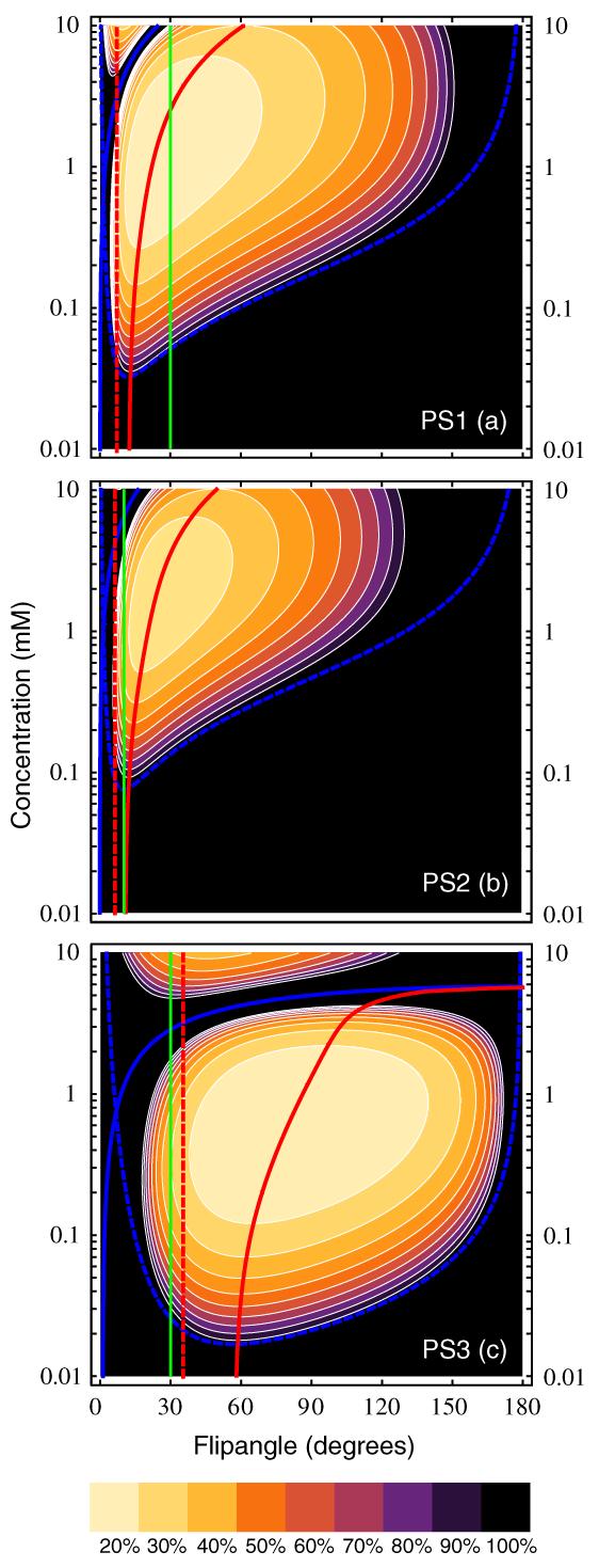
Contour plots of the dependence of relative concentration uncertainty from equation (16b) on both C and flip angle, assuming that measurement noise is independent of α, for PS1 (panel (a)), PS2 (panel (b)) and PS3 (panel (c)). Tissue parameters were for skeletal muscle, from table 3. Contours (thin white lines) are drawn at 10% intervals, with the outermost contour corresponding to ∊rel = 100%. Cdet is shown by the thick dashed blue line, Cmax by the thick solid blue line, the Ernst angle, αE, by the thick dashed red line, and the optimal flip angle, αopt, by the thick solid red line. The nominal flip angle for each pulse sequence from table 2 is indicated by the solid green line.
Curves of ∊rel after optimization of α for a contrast concentration of 1.0 mM in skeletal muscle and for the NB given in the previous paragraph are shown in figure 11. Comparison with pre-optimization curves from figure 4 shows moderate improvement for PS1 over most of the concentration range shown, although the slightly decreased Cmax leads to some increase in uncertainty for concentrations above ≈ 6 mM. In contrast, both PS2 and PS3 show dramatic decreases in relative uncertainty over virtually the entire concentration range from 0-10 mM. Percent change in effective SNR resulting from optimization of flip angle, given by (∊rel(α) - ∊rel(αopt))/∊rel(αopt, is given in table 6 for concentrations of 0.1, 0.5, 1.0 and 5.0 mM.
Figure 11.

Relative concentration measurement uncertainty from equation (16b) for PS1 (panels (a), (b)), PS2 (panels (c), (d)) and PS3 (panels (e), (f)) as in figure 4 except with flip angle set at the optimal value, αopt, for skeletal muscle at C = 1.0 mM. NB was set to the values from figure 10.
Table 6.
Percent change in effective SNR for PS1-PS3 resulting from optimizing flip angle for skeletal muscle at C = 1.0 mM and increasing NB to give 2 min of baseline scanning before injection
| C | 0.1 mM | 0.5 mM | 1.0 mM | 5.0 mM | |
|---|---|---|---|---|---|
| PS1 | Arterial blood | +53% | +80% | +86% | +37% |
| Skeletal muscle | +45% | +62% | +69% | +29% | |
| Liver tissue | +33% | +37% | +40% | +10% | |
| PS2 | Arterial blood | -15% | +39% | +90% | +697% |
| Skeletal muscle | -6% | +48% | +104% | +834% | |
| Liver tissue | +17% | +70% | +130% | +1166% | |
| PS3 | Arterial blood | +33% | +140% | +238% | ⋆ |
| Skeletal muscle | +74% | +205% | +327% | ⋆ | |
| Liver tissue | +183% | +351% | +527% | ⋆ |
Concentration exceeds Cmax.
Optimizing the flip angle for PS1 provides 40-86% improvement in effective signal-to-noise ratio over the 0.5-1.0 mM concentration range despite the relatively good initial choice of α, with 33-53% improvement at 0.1 mM and 10-37% improvement at 5 mM concentrations. Optimizing the flip angle of PS2 has an even larger effect, increasing effective SNR by 39-1166% for concentrations of 0.5 mM or greater, with the most dramatic increases at C = 5.0 mM. There is some loss in accuracy for this pulse sequence at C = 0.1 mM, but the relative uncertainty here is large enough that these concentrations would be difficult to measure in any case. Similar improvement is noted for PS3, where optimizing flip angle from the nominal value of 30° (close to the pre-contrast Ernst angle for blood) increased effective SNR at all measurable concentrations, with gains ranging from 33-527%. The accuracy of the optimized PS3 curves exceeds or is comparable to the optimized PS1 curves over most of the range from 0-2 mM, in contrast to the clearly inferior performance of this pulse sequence prior to optimization, and Cmax has increased to nearly 4 mM. As visible in figure 3, PS3 has a maximum possible saturation concentration of roughly 6 mM (at α = 180°), so no amount of optimization of flip angle (without changing repetition and/or echo time) will enable measurement of higher contrast concentrations. This is not likely to pose difficulties as long as AIF is not to be measured, as such high contrast concentrations are almost never attained in tissues.
4.3. In vivo measurements
Figure 12 shows representative AIF and tissue curves from three patients, with patient 1 in 12(a) and (b), patient 2 in 12(c) and (d), and patient 3 in 12(e) and (f). Contrast concentration computed from the measured values of Ξ by numerically solving the full nonlinear expression in equation (4) is indicated by the open circles. Thick solid black lines indicate the result of fitting the concentration curves to either an empirical model function (for AIFs, equation (A.1) in the appendix) or to the extended Kety model given in equation (38) using the measured AIF (for tissue curves). Solid gray bars indicate the ± 2Cdet detection window calculated from equation (19). Dark gray lines show fit curves ±∊abs, while light gray lines show fit curves ±2∊abs, where absolute concentration uncertainties were calculated from equation (16a). AIF data in figures 12(a), (c), and (e) include much magnified plots of the pre-contrast baseline scan data points in the insets. Estimated uncertainty curves show excellent agreement with the observed variability in the measured AIF data and predicted detection thresholds agree well with noise in the baseline measurements for all three patients, demonstrating that we are in the regime where the approximations involved in derivation of equation (19) are valid. The tissue curves shown in figures 12(b), (d) and (f) show comparably good agreement. A few outlier data points, likely arising from patient motion, are clearly visible, particularly in figures 12(c), (d) and (f).
Figure 12.

A comparison of measured and predicted uncertainties in concentration for the arterial input function (panels (a), (c) and (e)) and tumor tissue (panels (b), (d) and (f)) for three human study participants (patient 1 in panels (a), (b), patient 2 in panels (c), (d) and patient 3 in panels (e), (f)). Measured concentrations are shown by the open circles. Solid gray bars indicate the predicted ±2Cdet concentration detection window. The solid black line shows regression to a model AIF (input function curves) or the extended Kety model (tissue curves), as described in the text. Predicted ± ∊abs and ±2∊abs error bars are indicated by the dark and light gray lines, respectively. The insets in the AIF panels show magnified views of the pre-contrast baseline measurements.
We quantitatively estimate the concentration measurement uncertainty from our in vivo data by computing the root-mean-square (RMS) residual difference between the measured concentrations and the model fits, which we denote . This estimate should provide an independent proxy for true concentration uncertainty as long as the model function fits the measured time-concentration curves accurately, but will overestimate true concentration uncertainty when the model fit is poor. A spatial map of is shown for a single slice of data from patient 2 in figure 13(a). Figure 13(b) shows the corresponding map of ∊abs as determined using equation (16a) with the nominal pulse sequence parameters from table 1 and SNR determined from the ratio of pre-contrast signal to pre-contrast signal variance. Noise in the Ξabs map arises entirely from uncertainty in the estimated SNR. Both panels, which are plotted on identical color scales, agree well, providing additional support for the accuracy of equation (16a) for prediction of concentration measurement uncertainties. Comparable agreement is seen in the other two patients; the average relative difference between and ∊abs is 3.6 ± 27.6% for patient 1, 12.2 ± 34.1% for patient 2 and 6.4 30.2% for patient 3. The small positive bias stems from voxels which are not well fit by the extended Kety model we used. The standard deviation is relatively consistent across patients, indicating that our theoretical expression for uncertainty is capable of predicting concentration measurement uncertainties with an accuracy of roughly 30%.
Figure 13.
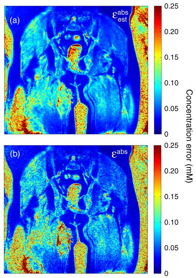
A map of the concentration measurement uncertainty estimated from the RMS residual values from model regression , as described in the text, is shown in panel (a). The corresponding map of ∊abs as predicted using equation (16a) is shown in panel (b). Both maps are derived from a single coronal section of data across the pelvis and proximal thighs from patient 2, plotted on a color scale covering the range 0 ≤ ∊abs ≤ 0.25 mM. Patchy regions corresponding to increased contrast uptake in a recurrent Ewing’s sarcoma are visible in the proximal right thigh.
5. Discussion
Dynamic contrast-enhanced MRI experiments are generally signal-starved, and the use of sub-optimal pulse sequence parameters needlessly amplifies the compromises between SNR, and spatial and temporal resolution that must be made in DCE-MRI data acquisition. The inverse proportionality between ∊rel and SNR implies that decreasing concentration uncertainty is precisely equivalent to increasing signal-to-noise ratio, in the absence of other considerations such as partial volume or sampling time effects. Therefore, if the concentration uncertainty term is regarded as negligible relative to other anticipated sources of uncertainty, it should be possible to sacrifice SNR to achieve better spatial or temporal resolution. Conversely, if the contribution of concentration uncertainty is too large, it can be reduced by increasing voxel volume or acquisition time. In either case, selection of suboptimal imaging parameters will lead to concentration measurements that are either unnecessarily noisy or have unnecessarily low spatial or temporal resolution.
There are several practical applications of the work presented here. First, the competing requirements of spatial coverage, voxel size, and sampling time in DCE-MRI experiments lead to an inevitable trade-off between SNR and spatial and temporal resolution. The expressions derived in this paper make the impact of these compromises explicit, allowing one to optimize imaging parameters to maximize measurement accuracy. Second, Cdet and Cmax define a window that spans the range of concentrations that may be measured. Ensuring that this window covers the expected range is essential in DCE-MRI experiments, particularly those where the arterial input function (AIF) is to be measured. Because peak blood contrast concentrations generally reach 5-10 mM for bolus injection (Parker et al 2006), while tissue concentrations typically lie in the 0-2 mM range, the chosen imaging parameters must strike an acceptable compromise that allows sufficiently accurate measurement of bolus concentration while at the same time minimizing uncertainties in tissue concentration measurement. In addition, while in vivo measurement of AIF is generally regarded as the optimal methodology for DCE-MRI experiments, it is not uncommon in clinical and animal studies to use population-averaged estimates for the AIF instead, so that only tissue concentration measurements are of interest. In these cases, the use of imaging protocols designed for AIF measurement will almost certainly provide suboptimal accuracy because of the much lower peak concentrations. Optimization of pulse sequence parameters to maximize sensitivity to lower concentrations of contrast agent using the methods described here can potentially lead to sizable improvements in measurement accuracy. Third, nonlinearity in the SPGR signal-concentration relationship is known to lead to significant uncertainties in PK parameter estimates (Heilmann et al 2006). Our expression for concentration measurement uncertainty includes the effects of nonlinearity explicitly, and can be used as input to pharmacokinetic regression models to give accurate estimates of the resulting uncertainties in PK parameters. Finally, uncertainty in the true values of α, T1,0, r1 and can result in concentration-dependent biases in time curves measured by DCE-MRI. Because these biases are systematic, they have the potential to impact PK model-derived kinetic parameters if they are large. The expressions provided here enable this effect to be modeled, allowing the uncertainty in PK parameters to be accurately estimated.
Sequence optimization by minimization of relative uncertainty with respect to flip angle has the potential to achieve large improvement in concentration measurement uncertainty with essentially no cost. Because optimal flip angle depends on tissue type and on concentration, it is not possible to define a single, global optimum value, so it is important for the choice of flip angle to be guided by realistic estimates of the range of pre-contrast longitudinal relaxation times and concentrations to be measured. Tissue and tumor longitudinal relaxation times are well known, and are almost invariably within the range of 500-1500 ms before contrast administration. Constraining the expected concentration range is somewhat more difficult due to variations in injection protocol, bolus volume, tissue type, etc, but in most clinical studies in humans the peak blood contrast concentration is less than 5-10 mM and tissue concentrations rarely exceed 1-2 mM. The concentration and flip angle dependence of ∊rel is relatively weak near the minimum, as is its dependence on T1,0, so optimization of flip angle for one tissue type and concentration should not result in uncertainties that vary dramatically for reasonably similar T1,0 and/or C values. Nevertheless, the increasing steepness of the error surface for decreasing flip angles makes it safest to err on the side of larger flip angles. It is also important to note that performing measurements of concentration at the Ernst angle leads to poor performance as αE is generally much smaller than αopt (see figure 10).
A good heuristic for optimizing pulse sequence parameters is that Cmax should be at least 150-200% of the largest concentration to be measured. Within this constraint, flip angle can be optimized for the tissue with the smallest T1,0 value expected (because Cmax decreases with decreased T1,0) for a concentration somewhere in the range of anticipated tissue concentrations. The former constraint ensures that no measurement will be too close to the region of greatest error amplification and that the error curves will be relatively flat, while the latter ensures that measurements will be nearly optimal in the tissues of interest. αopt can be computed by numerical minimization of the relative concentration uncertainty given in equation (16b) with respect to flip angle, at constant noise, using standard nonlinear optimization software. However, care must be taken to choose a reasonable starting guess because of the presence of a second minimum corresponding to the -weighted regime. An initial guess of αguess = 2 cos-1(E1) appears to give reasonable results in most cases. Non-tumor applications of quantitative contrast-enhanced imaging such as articular cartilage and multiple sclerosis have much less stringent acquisition time constraints due to much lower contrast enhancement rates, but also often demonstrate substantially lower peak concentration values. For these applications, measurement of the bolus input is not generally critical, so flip angle could be tuned to maximize sensitivity to low concentrations instead.
While patient motion and acquisition time limit the maximum number of pre-contrast baseline scans that can be measured, it is often possible to achieve non-negligible gains in effective SNR with reasonable increases in baseline scan time. The potential for such gains will depend on details of the anatomy to be measured and other aspects of the study being performed. In anatomic regions that can be adequately stabilized such as the head or extremities, motion due to respiration and/or pulsatility is minimal and extending the period of baseline scanning is likely to be beneficial. In contrast, even if image registration methods are used, motion-induced variability will likely limit the benefits of increased NB in abdominal or thoracic DCE-MRI studies. Longer baseline scans should also be beneficial in experiments on anesthetized animals where the motion is controlled and acquisition time limitations are significantly less stringent. Assuming that physiological sources of motion are not limiting, equation (17) can be used to assess whether increasing NB will provide sufficient improvement in measurement accuracy to justify the added acquisition time.
Values of flip angle and T1,0 are generally either measured once before the beginning of dynamic data acquisition or are assumed. Unlike concentration uncertainty stemming from finite signal-to-noise ratio and pre-contrast measurement time, uncertainties in α and T1,0 will be temporally correlated for each voxel, so they will result in biasing of the concentration-time curves. If α and T1,0 are measured by an unbiased method, the bias should vary randomly from pixel to pixel, while assumed values will lead to strong spatial correlation of biases. For region-of-interest analyses that average concentration curves over many voxels, if α and T1,0 have been measured the residual biases arising from misestimation in those measurements should be uncorrelated between voxels and the bias terms may be treated as uncertainties in this case. Because the biases demonstrate nonlinear behavior with concentration, becoming amplified as C → Cmax, they result in changes to both the scale and the shape of contrast concentration curves, potentially resulting in subtle biases in parameters determined from PK modeling. Values of the contrast relaxivities r1 and are generally assumed to be equivalent to those measured in vitro, despite some evidence suggesting significant deviations from those values in vivo (Stanisz and Henkelman 2000). Fortunately, the nonlinearity in relaxivity bias is restricted to concentrations quite close to Cmax, with the r1 bias being nearly linear and the bias being very small over a wide range, so misestimation of contrast relaxivity will primarily scale the measured curves. While scaling will impact absolute quantification, it is probably of little practical significance for comparative clinical studies using consistent relaxivity estimates.
Comparison of concentration-time curves measured in vivo with our predictions for concentration uncertainty shows that the high-frequency variability is accurately bounded by the theoretical uncertainties in all three patients for both AIF and tissue curves, with the exception of a few outlier points visible in figure 12. Our expression for Cdet also accurately models the observed pre-contrast variability in these data. Maps of estimated and predicted concentration uncertainties show good overall agreement between the estimated and theoretically predicted uncertainties. Statistics on the average relative difference between the estimated and predicted uncertainties from patient data indicate that the theoretical predictions of equation (16a) should be accurate to better than 30% in vivo for reasonable acquisition parameters. One limitation of the present analysis is that, while the main equations derived in the theory section are applicable to arbitrary concentration-dependent relaxation rates, we have not considered potential deviation from the FXL here. The investigation of the impact of transcytolemmal exchange in tissues on contrast quantification error and systematic biases would be an interesting area for further research.
6. Conclusions
We have derived a number of useful theoretical results from analysis of contrast-dependent signal enhancement for SPGR pulse sequences. These results have been tested both in vitro and in vivo, and demonstrate good agreement with measured data. In particular, we show that it is possible to accurately predict concentration measurement uncertainties directly from pulse sequence parameters and measured signal-to-noise ratio. For clinically relevant pulse sequence parameters and contrast doses, the optimization of acquisition parameters (primarily flip angle and number of baseline measurements) in DCE-MRI protocols can lead to significant gains in effective SNR as well as decreased sensitivity to biases arising from misestimation of flip angle and/or pre-contrast longitudinal relaxation time. Use of the methods described here in the planning of DCE-MRI experiments should facilitate selection of imaging pulse sequence parameters that provide nearly optimal sensitivity for concentration quantification and enable accurate estimation of uncertainties in concentration measurements.
Acknowledgments
MCS would like to thank the National Institute for Biomedical Imaging and Bioengineering for its support of this work through the K25 Career Development Award #5K25EB005077-03. The authors would like to acknowledge Drs Edward DiBella, Eun-Kee Jeong, Eugene Kholmovsky, Glen Morrell, Frederic Noo and June Taylor for stimulating conversations and helpful comments.
Appendix
The model form used for fitting measured arterial input functions is given by
| (A.1) |
which is the sum of three normalized gamma variate curves,
| (A.2) |
and a sigmoid curve,
| (A.3) |
where t = 0 corresponds to the actual injection time, Γ(α) is the complete gamma function and γ (α, x) is the lower incomplete gamma function. The number of free parameters is reduced by the following constraints: Δ1 = Δ2 = Δ3 = Δ0, α2 = α3 = α0, and τ3 = τ0. For the model AIF shown in figure 7, the parameters used were A0 = 0.8152, A1 = 5.8589, A2 = 0.9444, A3 = 0.4888, Δ0 = 0.1563 min, α0 = 7.9461, α1 = 2.5393, τ1 = 0.04286 min, τ2 = 0.06873 min, τ3 = 0.1400 min and T = 9.6319 min.
References
- Batchelor TT, et al. AZD2171, a pan-VEGF receptor tyrosine kinase inhibitor, normalizes tumor vasculature and alleviates edema in glioblastoma patients. Cancer Cell. 2007;11:83–95. doi: 10.1016/j.ccr.2006.11.021. [DOI] [PMC free article] [PubMed] [Google Scholar]
- Bernstein MA, King KF, Zhou XJ. Handbook of MRI Pulse Sequences. Elsevier; Amsterdam: 2004. p. 587. chapter 14. [Google Scholar]
- Buckley DL. Uncertainty in the analysis of tracer kinetics using dynamic contrast-enhanced T1-weighted MRI. Magn. Reson. Med. 2002;47:601–6. doi: 10.1002/mrm.10080. [DOI] [PubMed] [Google Scholar]
- Collins DJ, Padhani AR. Dynamic magnetic resonance imaging of tumor perfusion. Approaches and biomedical challenges. IEEE Eng. Med. Biol. Mag. 2004;23:65–83. doi: 10.1109/memb.2004.1360410. [DOI] [PubMed] [Google Scholar]
- Conturo TE, Akbudak E, Kotys MS, Chen ML, Chun SJ, Hsu RM, Sweeney CC, Markham J. Arterial input functions for dynamic susceptibility contrast MRI: Requirements and signal options. J. Magn. Reson. Imaging. 2005;22:697–703. doi: 10.1002/jmri.20457. [DOI] [PubMed] [Google Scholar]
- Dale BM, Jesberger JA, Lewin JS, Hillenbrand CM, Duerk JL. Determining and optimizing the precision of quantitative measurements of perfusion from dynamic contrast enhanced MRI. J. Magn. Reson. Imaging. 2003;18:575–84. doi: 10.1002/jmri.10399. [DOI] [PubMed] [Google Scholar]
- Deichmann R. Fast high-resolution T1 mapping of the human brain. Magn. Reson. Med. 2005;54:20–7. doi: 10.1002/mrm.20552. [DOI] [PubMed] [Google Scholar]
- Deoni SCL, Rutt BK, Peters TM. Rapid combined T1 and T2 mapping using gradient recalled acquisition in the steady state. Magn. Reson. Med. 2003;49:515–26. doi: 10.1002/mrm.10407. [DOI] [PubMed] [Google Scholar]
- Fram EK, Herfkens RJ, Johnson GA, Glover GH, Karis JP, Shimakawa A, Perkins TG, Pelc NJ. Rapid calculation of T1 using variable flip angle gradient refocused imaging. Magn. Reson. Imaging. 1987;5:201–8. doi: 10.1016/0730-725x(87)90021-x. [DOI] [PubMed] [Google Scholar]
- Heilmann M, Kiessling F, Enderlin M, Schad LR. Determination of pharmacokinetic parameters in DCE MRI: Consequence of nonlinearity between contrast agent concentration and signal intensity. Invest. Radiol. 2006;41:536–43. doi: 10.1097/01.rli.0000209607.99200.53. [DOI] [PubMed] [Google Scholar]
- Jackson A, Buckley D, Parker GJM. Dynamic Contrast-Enhanced Magnetic Resonance Imaging in Oncology. Springer; Berlin: 2003. [Google Scholar]
- Kershaw LE, Buckley DL. Precision in measurements of perfusion and microvascular permeability with T1-weighted dynamic contrast-enhanced MRI. Magn. Reson. Med. 2006;56:986–92. doi: 10.1002/mrm.21040. [DOI] [PubMed] [Google Scholar]
- Kiselev VG. Effect of magnetic field gradients induced by microvasculature on nmr measurements of molecular self-diffusion in biological tissues. J. Magn. Reson. 2004;170:228–35. doi: 10.1016/j.jmr.2004.07.004. [DOI] [PubMed] [Google Scholar]
- Kruger G, Glover GH. Physiological noise in oxygenation-sensitive magnetic resonance imaging. Magn. Reson. Med. 2001;46:631–7. doi: 10.1002/mrm.1240. [DOI] [PubMed] [Google Scholar]
- Landis CS, Li X, Telang FW, Molina PE, Palyka I, Vetek G, Springer CS., Jr Equilibrium transcytolemmal water-exchange kinetics in s keletal muscle in vivo. Magn. Reson. Med. 1999;42:467–78. doi: 10.1002/(sici)1522-2594(199909)42:3<467::aid-mrm9>3.0.co;2-0. [DOI] [PubMed] [Google Scholar]
- Leach MO, et al. Assessment of antiangiogenic and antivascular therapeutics using MRI: Recommendations for appropriate methodology for clinical trials. Br. J. Radiol. 2003;76(Spec No 1):S87–91. doi: 10.1259/bjr/15917261. [DOI] [PubMed] [Google Scholar]
- Nkongchu K, Santyr G. An improved 3-D Look-Locker imaging method for T(1) parameter estimation. Magn. Reson. Imaging. 2005;23:801–7. doi: 10.1016/j.mri.2005.06.009. [DOI] [PubMed] [Google Scholar]
- Parker DL, Gullberg GT. Signal-to-noise efficiency in magnetic resonance imaging. Med. Phys. 1990;17:250–7. doi: 10.1118/1.596503. [DOI] [PubMed] [Google Scholar]
- Parker GJM, Roberts C, Macdonald A, Buonaccorsi GA, Cheung S, Buckley DL, Jackson A, Watson Y, Davies K, Jayson GC. Experimentally-derived functional form for a population-averaged high-temporal-resolution arterial input function for dynamic contrast-enhanced MRI. Magn. Reson. Med. 2006;56:993–1000. doi: 10.1002/mrm.21066. [DOI] [PubMed] [Google Scholar]
- Pickles MD, Lowry M, Manton DJ, Gibbs P, Turnbull LW. Role of dynamic contrast enhanced MRI in monitoring early response of locally advanced breast cancer to neoadjuvant chemotherapy. Breast Cancer Res. Treat. 2005;91:1–10. doi: 10.1007/s10549-004-5819-2. [DOI] [PubMed] [Google Scholar]
- Rijpkema M, Kaanders JH, Joosten FB, van der Kogel AJ, Heerschap A. Method for quantitative mapping of dynamic MRI contrast agent uptake in human tumors. J. Magn. Reson. Imaging. 2001;14:457–63. doi: 10.1002/jmri.1207. [DOI] [PubMed] [Google Scholar]
- Rohrer M, Bauer H, Mintorovitch J, Requardt M, Weinmann H-J. Comparison of magnetic properties of MRI contrast media solutions at different magnetic field strengths. Invest. Radiol. 2005;40:715–24. doi: 10.1097/01.rli.0000184756.66360.d3. [DOI] [PubMed] [Google Scholar]
- Schmid VJ, Whitcher BJ, Yang G-Z, Taylor NJ, Padhani AR. Statistical analysis of pharmacokinetic models in dynamic contrast-enhanced magnetic resonance imaging. Med. Image Comput. 2005;8:886–93. doi: 10.1007/11566489_109. [DOI] [PubMed] [Google Scholar]
- Stanisz GJ, Henkelman RM. Gd-DTPA relaxivity depends on macromolecular content. Magn. Reson. Med. 2000;44:665–7. doi: 10.1002/1522-2594(200011)44:5<665::aid-mrm1>3.0.co;2-m. [DOI] [PubMed] [Google Scholar]
- Stanisz GJ, Odrobina EE, Pun J, Escaravage M, Graham SJ, Bronskill MJ, Henkelman RM. T1, T2 relaxation and magnetization transfer in tissue at 3T. Magn. Reson. Med. 2005;54:507–12. doi: 10.1002/mrm.20605. [DOI] [PubMed] [Google Scholar]
- Tofts PS. Modeling tracer kinetics in dynamic Gd-D TPA MR imaging. J. Magn. Reson. Imaging. 1997;7:91–101. doi: 10.1002/jmri.1880070113. [DOI] [PubMed] [Google Scholar]
- Tofts PS, et al. Estimating kinetic parameters from dynamic contrast-enhanced T(1)-weighted MRI of a diffusable tracer: Standardized quantities and symbols. J. Magn. Reson. Imaging. 1999;10:223–32. doi: 10.1002/(sici)1522-2586(199909)10:3<223::aid-jmri2>3.0.co;2-s. [DOI] [PubMed] [Google Scholar]
- Treier R, Steingoetter A, Fried M, Schwizer W, Boesiger P. Optimized and combined T1 and B1 mapping technique for fast and accurate T1 quantification in contrast-enhanced abdominal MRI. Magn. Reson. Med. 2007;57:568–76. doi: 10.1002/mrm.21177. [DOI] [PubMed] [Google Scholar]
- van Osch MJP, van der Grond J, Bakker CJG. Partial volume effects on arterial input functions: Shape and amplitude distortions and their correction. J. Magn. Reson. Imaging. 2005;22:704–9. doi: 10.1002/jmri.20455. [DOI] [PubMed] [Google Scholar]
- Workie DW, Dardzinski BJ, Graham TB, Laor T, Bommer WA, O’Brien KJ. Quantification of dynamic contrast-enhanced MR imaging of the knee in children with juvenile rheumatoid arthritis based on pharmacokinetic modeling. Magn. Reson. Imaging. 2004;22:1201–10. doi: 10.1016/j.mri.2004.09.006. [DOI] [PubMed] [Google Scholar]
- Yankeelov TE, Rooney WD, Li X, Springer CS., Jr Variation of the relaxographic ‘shutter-speed’ for transcytolemmal water exchange affects the CR bolus-tracking curve shape. Magn. Reson. Med. 2003;50:1151–69. doi: 10.1002/mrm.10624. [DOI] [PubMed] [Google Scholar]
- Yankeelov TE, et al. Integration of quantitative DCE-MRI and ADC mapping to monitor treatment response in human breast cancer: initial results. Magn. Reson. Imaging. 2007;25:1–13. doi: 10.1016/j.mri.2006.09.006. [DOI] [PMC free article] [PubMed] [Google Scholar]
- Yarnykh VL. Actual flip-angle imaging in the pulsed steady state: a method for rapid three-dimensional mapping of the transmitted radiofrequency field. Magn. Reson. Med. 2007;57:192–200. doi: 10.1002/mrm.21120. [DOI] [PubMed] [Google Scholar]