

Abstract
Abnormal cerebrospinal fluid (CSF) flow is suspected to be a contributor to the pathogenesis of neurodegenerative diseases such as Alzheimer's through the accumulation of toxic metabolites, and to the malfunction of intracranial pressure regulation, possibly through disruption of neuroendocrine communication. For the understanding of transport processes involved in either, knowledge of in vivo CSF dynamics is important. We present a three-dimensional, transient, subject-specific computational analysis of CSF flow in the human cranial subarachnoid space (SAS) based on in vivo magnetic resonance imaging. We observed large variations in the spatial distribution of flow velocities with a temporal peak of 5 cm s−1 in the anterior SAS and less than 4 mm s−1 in the superior part. This could reflect dissimilar flushing requirements of brain areas that may show differences in susceptibility to pathological CSF flow. Our methods can be used to compare the transport of metabolites and neuroendocrine substances in healthy and diseased brains.
Keywords: cerebrospinal fluid, subarachnoid space, intracranial pressure regulation, Alzheimer's disease, porous media, magnetic resonance imaging
1. Introduction
The cerebrospinal fluid (CSF) not only provides mechanical protection to the central nervous system, but also acts as a transport medium for nutrients, neuroendocrine substances and for the removal of toxic metabolites, preserving the chemical environment of the brain (Davson et al. 1987). As outlined in the second part of this work (Holman et al. 2010), it is hypothesized that the disruption of CSF flow may be linked to neurodegenerative diseases such as Alzheimer's through disturbed regulation of intracranial pressure, through accumulation of toxic metabolites or through a combination of both (Segal 2000; Stopa et al. 2001; Kivisakk et al. 2003; Silverberg et al. 2003; Abbott 2005; Johanson et al. 2005).
The accumulation of any substance transported through the CSF is governed to a large extent by the pulsatile dynamics of this fluid. Surprisingly, little detail is known about CSF flow. This can be attributed to the fact that potentially accurate invasive flow measurements necessarily alter its motion, and that non-invasive studies are limited in resolution and accuracy, except in areas of well-defined shape with CSF motion along a predominant axis such as in the aqueduct of Sylvius, in the superior part of the spinal subarachnoid space (SAS) and, to a certain extent, in some planes within the various cranial cisterns. Magnetic resonance imaging (MRI) velocimetry is currently the most widely used technique to study the CSF flow non-invasively (Feinberg & Mark 1987; Enzmann & Pelc 1992; Poncelet et al. 1992).
Using three-dimensional computational fluid dynamics (CFD), it is possible to reconstruct the velocity field in the CSF space. This has been done for parts of the ventricular system, the spinal SAS and the inferior cranial SAS, but not for the remainder of the cranial SAS that poses serious modelling challenges owing to its complex anatomy spanning multiple length scales (Jacobson et al. 1996; Aroussi et al. 2000; Loth et al. 2001; Stockman 2006; Kurtcuoglu et al. 2007a; Gupta et al. 2009). This includes the spongy framework of trabeculae, which are delicate tissue filaments that protrude through the meninges into the SAS (Killer et al. 2003a). CSF is produced in the choroid plexus and is absorbed through the arachnoid granulations (AGs) (Haroun et al. 2007; Weller et al. 2009), extra-cranial lymphatic pathways (Johnston 2003) and possibly through additional intraparenchymal routes (Greitz et al. 1997). The drainage through the lymphatic pathways is well validated in mammals other than man, but there is no consensus on the relative importance of lymphatic CSF drainage compared with absorption through the AGs in humans, which is the traditionally accepted route (Koh et al. 2005; Weller et al. 2009). Despite the paucity of evidence supporting the AGs as the sole CSF absorption route, we only take into account this pathway by way of convenience, since more quantitative data on absorption through the AGs are available than on the lymphatic pathway. We show in §4 that this simplification will not influence the reported results substantially. With an average diameter of approximately 300 µm (Upton & Weller 1983), the AGs are well below the resolution limit of current clinical MRI units, and thus have to be modelled based on ex vivo (Grzybowski et al. 2007) and in vitro (Grzybowski et al. 2006; Holman et al. 2010) data.
In the work at hand, we use CFD to compute and analyse the flow in the cranial SAS based on in vivo anatomic and velocimetric MRI data of a healthy male volunteer (figure 1). We take into account the distribution of AGs based on ex vivo data gathered from 35 human brains (Grzybowski et al. 2007) and estimate the CSF outflow rate through the AGs again using in vivo MRI flow measurements. We model the influence of the trabecular framework using a previously described anisotropic porous model (Gupta et al. 2009). In that work, we investigated CSF flow in the superior spinal and inferior cranial SAS and the fourth ventricle. These areas are smaller than the here covered superior cranial SAS, they do not contain any AGs and they have less intricate anatomic features.
Figure 1.

(a) Anatomic MRI images of the cranial space; (b) segmentation and reconstruction of the SAS and the brain structures; (c) three-dimensional brain anatomy; (d) three-dimensional SAS anatomy; (e) detailed anatomy of the SAS showing sulci.
We show in the work at hand that there are large spatial variations in the velocity distribution in the cranial SAS that will influence the transport behaviour of toxic metabolites and neuroendocrine and other substances released into the CSF. Assuming there are physiological reasons for these variations, we hypothesize that not all regions of the brain will be affected with the same severity by disrupted CSF flow.
2. Material and methods
2.1. SAS anatomy and CSF flow acquisition
T2-weighted MRI scans were performed on a 25-year-old healthy male volunteer using a whole-body 3T MRI scanner (Achieva, Philips Medical Systems, Best, The Netherlands). The in-plane resolution of the scans was 0.45 × 0.45 mm and the slice spacing was 0.6 mm. The details of the MRI acquisition sequence are presented in Gupta et al. (2009). The acquired images were manually segmented using Amira 4.1 (Mercury Computer Systems, San Diego, CA, USA) to obtain a three-dimensional representation of the SAS (figures 1 and 2). The voxel-based segmented structures were then converted to non-uniform rational B-spline surfaces in order to allow for efficient generation of a high-quality computational grid.
Figure 2.

(a) Rendering of the cranial SAS (opaque) and of the superior spinal SAS and fourth ventricle (transparent). (b) Cranial SAS novel to this work.
MRI velocimetry was used to acquire CSF velocity data at the inferior boundaries of the cranial SAS, i.e. in the pontine and cerebellomedullary cisterns. A phase contrast velocity mapping sequence combined with an ECG-triggered T1-weighted transient field echo read-out scheme was applied (Gupta et al. 2009). In order to maximize the velocity signal-to-noise ratio, the phase-encoding velocity was adjusted so as to conform to the maximum velocity at the boundary. The phase-encoding velocity was set to 2 cm s−1 for the measurements in the cerebellomedullary cistern and to 4 cm s−1 for measurements in the pontine cistern. The measured profiles were manually phase-unwrapped, filtered with a filter mask of 5 × 5 pixels (Lim 1990) and then smoothed using cubic spline interpolation. Figure 3 shows the boundary velocity profiles at the measurement locations within the pontine and cerebellomedullary cisterns during one cardiac cycle.
Figure 3.

Velocities measured with MRI normal to the boundaries in (a) cerebellomedullary cistern and (b) pontine cistern during one cardiac cycle of period T. Velocities are shown at uniform intervals of T/5.
2.2. Distribution and hydraulic conductivity of arachnoid granulations
The detailed characterization of the AGs' topography and morphology is currently not possible with any in vivo measurement technique. Grzybowski et al. (2007) characterized the AG distribution in the superior sagittal sinus based on en face digital images of 35 human brain samples. For the present analysis, areas of AGs that were present in more than 10 per cent of the analysed brains in Grzybowski et al. (2007) were mapped to the current anatomic geometry. The surface area occupied by the AGs, AAG, amounted to 114 mm2, which is approximately 0.29 per cent of the total brain surface area. It is to be noted that while CSF drainage may take place through several pathways, in our model all CSF absorption occurs exclusively through the AGs clearing into the superior sagittal sinus.
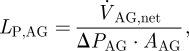
The most important parameter that governs CSF outflow through the granulations is their hydraulic conductivity (Albeck et al. 1991; Eklund et al. 2007; Grzybowski et al. 2007). Hydraulic conductivity, LP,AG, is a measure of the amount of CSF that flows through a unit cross-sectional area of the granulation surface as a result of a unit pressure drop across that surface,
 |
2.1 |
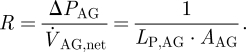
where ΔPAG is the total pressure drop across the AG surface and  is the net outflow through the AGs. Alternatively, the resistance to cerebrospinal outflow can be defined as
 |
2.2 |
We modelled the AGs as differential pressure valves that respond to the pressure difference ΔPAG between the SAS and the superior sagittal sinus, allowing only unidirectional flow out of the SAS. Estimates of ΔPAG across the granulation membranes are published in Davson et al. (1987) and Grzybowski et al. (2006) as ΔPAG = 3.15 mmHg (420 Pa).
2.3. Computational model
We have reconstructed CSF motion in the cranial SAS using a finite-volume (FV) CFD approach (Versteeg & Malalasekra 1996). The fundamental basis of this approach is the discretization of the governing fluid flow partial differential equations known as Navier–Stokes (NS) equations into a system of coupled algebraic equations that can be solved iteratively. While FV CFD is a computationally expensive technique, particularly when dealing with complex geometries, it is well validated and its ability to handle complex flows has been demonstrated in various research and industrial applications. In order to incorporate the effect of the trabecular morphology of the SAS into the calculations, the SAS was modelled as a porous medium by extension of the NS equations to the NS/Brinkman equations (Brinkman 1948). The permeability k of the SAS varies anisotropically throughout the domain. For its estimation, the porous SAS is assumed to feature an idealized morphology with straight cylindrical pillars representing the trabeculae extending perpendicularly from the pia to the arachnoid mater. This simplification allows for the application of a closed-form mathematical solution for the permeability in an arbitrary direction within the SAS for a given trabecular radius and porosity (Van der Westhuizen & Du Plessis 1994). For the current computations, we used an SAS porosity value of ε = 0.99 (Tada & Nagashima 1994) and a trabecular radius of r = 15 µm (Killer et al. 2003b). A detailed description of the derivation of the porous SAS model is given in Gupta et al. (2009).
CFD analysis requires the discretization of the SAS domain into a large number of small cells, within which pressure and velocity are approximately uniform. These cells define the computational grid. The presence of sulci and the wide range of length scales within the cranial SAS necessitate a very fine computational grid for accurate CFD computations. We modelled CSF as an incompressible, Newtonian fluid with the same density and viscosity as that of water at 37°C (Bloomfield et al. 1998; Kurtcuoglu et al. 2007b). The computations were performed using a commercial FV CFD solver Fluent 6.3 (Fluent Inc., Lebanon, NH, USA) on a high-quality computational grid consisting of 14 million cells. A discussion of the influence of the choice of computational grid on the reported results is presented in the electronic supplementary material, figure S7.
Velocity profiles obtained using MRI as described above were imposed at boundaries within the pontine and cerebellomedullary cisterns (figure 3). The measured profiles were first interpolated onto the computational grid and then interpolated in time in accordance with the temporal step size used for the transient computations. In order to take into account brain motion, an artificial transient volumetric flow rate,  , was imposed uniformly at the entire brain surface, with flow direction normal to the surface. This approach lets us avoid the exceedingly complex and computationally costly transient deformation of the computational grid, while still accounting for spatially averaged CSF motion induced by brain deformation. This artificial volumetric flow rate was determined as
| 2.3 |
where  and
and  are the transient volumetric flow rates into the SAS domain at the boundaries in the pontine and cerebellomedullary cisterns, respectively, and
  is the net outflow through the AGs given by equation (2.4). The volumetric flow rates
  and
and  were obtained by integrating the spatial velocity profiles (acquired using velocimetric MRI as described above) over the respective boundary. The calculation of
  is shown in §3. The obtained spatially averaged transient brain surface deformation rate, calculated by dividing
  by the brain surface area, is shown in figure 4. The boundary conditions used in the current computational model are further summarized in table 1.
Figure 4.

Spatially averaged transient deformation rate of the cranial SAS at the brain surface and the corresponding volumetric flow rate used as the boundary condition.
Table 1.
Boundary conditions used for the flow calculations. The variation column indicates possible time and space dependence of the respective boundary condition. Pressure values are given relative to zero constant blood pressure in the superior sagittal sinus.
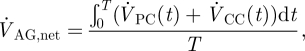
If we neglect absorption of CSF at locations other than the AGs, the net CSF produced within a cardiac cycle will equal the total outflow through the AGs,  , which can be expressed as
 |
2.4 |
where T is the time period of one cardiac cycle. Using equation (2.4),  evaluates to 0.47 ml min−1. With a pressure drop, ΔPAG, of 3.15 mmHg across the granulation membrane and an AG surface area of 114 mm2, the hydraulic conductivity of the granulations LP,AG is 130.9 µl min−1 mmHg−1 cm−2 (equation (2.1)). Correspondingly, the resistance, R, of the AGs to CSF outflow evaluates to 6.7 mmHg ml−1 min−1 (equation (2.2)). This high value is in good agreement with the results reported in Albeck et al. (1991) and Eklund et al. (2007) and is indicative of the fact that the mesothelial cell layer lining the AG surface offers high resistance to CSF outflow, thus limiting CSF drainage into the venous blood.
3. Results
We will refer to the space surrounding the parietal and superior frontal lobes of the cerebral cortex as the superior cranial SAS (figure 2). The space surrounding the frontal lobe and the temporal lobe including chiasmatic and interpeduncular cisterns will be referred to as the anterior cranial SAS. Inferior to the interpeduncular cistern is the pontine cistern, where CSF enters the cranial SAS through the left and right foramina of Luschka and through the spinal SAS. The posterior cranial SAS surrounds the occipital lobe, including the quadrigeminal cistern and the region below it. It also surrounds the cerebellum and extends up to the cerebellomedullary cistern.
Figures 5 and 6 and the movies in the electronic supplementary material visualize the CSF velocity and pressure field. With respect to velocity distribution, the cranial SAS can be divided into three distinct regions: (i) posterior cranial and superior cranial SASs, exhibiting low velocities with peak values less than 4 mm s−1 throughout the cardiac cycle, except in the vicinity of the cerebellomedullary cistern, where the peak velocity is 8.3 mm s−1; (ii) anterior cranial SAS, excluding chiasmatic and interpeduncular cisterns, exhibiting higher velocities than the posterior cranial and superior cranial spaces with absolute maximum velocity up to 1.3 cm s−1; (iii) chiasmatic, interpeduncular and pontine cisterns with maximum velocity up to 5 cm s−1. Table 2 presents various flow parameters at selected cross sections within the SAS. The stroke volume, SV, is obtained in two steps, first by determining the area under the transient volumetric flow-rate curve of the respective cross section for caudio-cranial (positive) and cranio-caudal (negative) flow rates, and then by taking the mean of the absolute value of these two areas. For the AGs, the stroke volume is calculated as the product of net volumetric flow rate through the granulations,  , and the time period, T, of the cardiac cycle.
Figure 5.

Relative pressure, P, contours in the SAS during one complete cardiac cycle. The pressure values are given with respect to the CSF outlet pressure, PCSF,outlet = ΔPAG + PSSS, where PSSS is the blood pressure in the superior sagittal sinus and ΔPAG is the pressure drop across the AGs.
Figure 6.

Velocity magnitude contours at cross sections of the cranial SAS at selected points in time within one cardiac cycle. Also shown are the stream traces of virtual massless particles injected arbitrarily within the domain at different points in time.
Table 2.
Volumetric flow rates, stroke volume, peak velocities, Reynolds numbers and Womersley parameters at key cross sections within the SAS. A, cross-sectional area; Dh, hydraulic diameter of the cross section; V1,max maximum volumetric flow rate in caudio-cranial direction; V2,max, maximum volumetric flow rate in cranio-caudal direction; SV, stroke volume; ϑpeak, peak flow velocity; Repeak, peak Reynolds number based on peak velocity, ϑpeak, and hydraulic diameter, Dh; α, Womersley parameter based on hydraulic radius (Dh/2).
| A (mm2) | Dh (mm) | V1,max (ml min−1) | V2,max (ml min−1) | SV (µl) | ϑpeak (cm s−1) | Repeak (−) | α (−) | |
|---|---|---|---|---|---|---|---|---|
| cross section at cerebellomedullary cistern | 159.1 | 6 | 17.9 | 6.44 | 38.64 | 0.83 | 72 | 9.91 |
| cross section at pontine cistern | 342.4 | 6.23 | 94.7 | 57.7 | 289.3 | 4.28 | 386 | 10.3 |
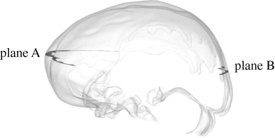
| plane A, anterior cranial SAS | 514 | 6.24 | 66.76 | 41.5 | 209.2 | 1.26 | 114 | 10.3 |
| plane B, posterior cranial SAS | 144.3 | 4.82 | 11.91 | 10.45 | 24.3 | 0.28 | 19.5 | 7.96 |
| AGs | 114 | — | 0.47 | 0 | 6.52 | — | — | — |
 |
||||||||
The peak Reynolds number, Repeak, is calculated based on the peak velocity, ϑpeak, and the hydraulic diameter, Dh = 4 ⋅ area/perimeter, of the respective cross section and is defined as
where ρ and μ are the CSF density and dynamic viscosity, respectively. The Reynolds number, Re, in general, is defined as the ratio of the inertial to the viscous forces present at a particular location within a given system. It is used as a measure of flow characteristics, where higher values indicate turbulent behaviour, lower values imply laminar flow and very low values indicate diffusive behaviour. The limits between these regimes are system dependent, but can be approximated as Re < 1 for the diffusive range, 1 < Re < 1000 for the laminar range and potentially turbulent dynamics for larger values. The maximum Reynolds number in the cranial SAS, Repeak = 386, was observed at the pontine boundary and lies well within the laminar range. Low Reynolds numbers with a peak value of 72 were observed in the posterior cranial SAS at the cerebellomedullary cistern boundary, and with a peak value of around 20 at plane B (see insert in table 2) in the posterior cranial SAS. The flow is primarily laminar in this region, with pockets of diffusive zones with Re < 1 such as in the quadrigeminal cistern.
The ratio of transient inertial forces to viscous forces can be studied by considering the Womersley parameter, α, which is defined as
 |
where T is the time period of the cardiac cycle. For small Womersley parameters (α < 1), the transient inertial forces are low, and hence the flow remains in phase with the driving pressure gradient. For larger Womersley parameters (α > 1), the transient inertial forces are high enough and the velocity profiles do not immediately follow the driving pressure gradient. As can be seen in table 2, the Womersley parameter is quite high in the entire treated domain, indicating strong transient inertial effects on the CSF flow field. Figure 5 shows the pressure distribution, P, at selected points within the cardiac cycle relative to the CSF outlet pressure PCSF,outlet = ΔPAG + PSSS, where PSSS is the blood pressure in the superior sagittal sinus and ΔPAG is the pressure drop across the AGs' surface. The absolute CSF pressure, Pabs, at any point within the domain can be determined as Pabs = P+ΔPAG + PSSS. The flow dynamics within a cardiac cycle can be described as follows.
At the beginning of the cardiac cycle, which is chosen to coincide with the R-peak of the electrocardiogram, CSF flows in the cranio-caudal direction in the anterior cranial SAS and in the pontine and cerebellomedullary cisterns. CSF flows in the cranio-caudal direction in the posterior cranial space surrounding the cerebellum and in the caudio-cranial direction in the SAS surrounding the occipital lobe. Thus, at the beginning of the cardiac cycle, CSF flows from the posterior cranial to the anterior cranial space with a net flow from the cranial SAS to the ventricular space and to the spinal SAS. This is caused, presumably, by the expansion of the lateral and third ventricles and the expansion of blood vessels in the SAS and beneath the pia mater, or by the compression of the SAS. The pressure, P, varies from −0.15 mmHg in the anterior cranial space to 0.04 mmHg in the posterior cranial space.
At around 20 per cent of the cardiac cycle, the flow in the entire space turns caudio-cranial. This is probably caused by the compression of blood vessels in or beneath the SAS or by the expansion of the SAS itself. In our computational model, both these effects are merged into a combined distensibility boundary condition at the brain surface and can, thus, not be distinguished (§2.3). The flow in this phase of the cardiac cycle features the highest velocities of the entire cycle. The pressure varies from 0 to 0.20 mmHg, with maximum value within the anterior cranial space.
At around 40 per cent of the cycle, CSF flows from the anterior cranial to the posterior cranial space with a net flow from the ventricular system to the cranial SAS. The reason for this is ventricular contraction, forcing CSF into the pontine cistern via the two foramina of Luschka. CSF in the pontine cistern is further carried upwards towards the superior cranial space, with the inertia of the CSF arriving from the spinal SAS. This phase of the cycle features very low velocities (less than 2 mm s−1) in the superior cranial and the posterior cranial SAS and a high inertia flow in the pontine cistern and in the anterior cranial SAS. The overall pressure varies from 0 to 0.11 mmHg, with maximum pressure still in the anterior cranial space.
The entire flow almost stagnates at around 60 per cent of the cardiac cycle. Peak velocities in the entire treated domain are less than 5 mm s−1 at this time and the pressure variation is small.
At approximately 80 per cent of the cardiac cycle, the flow closely resembles that at the beginning of the cycle. The absolute maximum velocity during this phase is 3 cm s−1, occurring within the pontine cistern. The velocities in the rest of the domain are very low. There is a decrease in the pressure in the anterior cranial space, while the pressures within the superior cranial and the posterior cranial SAS remain similar to those at 60 per cent of the cycle.
4. Discussion and limitations
The pressure in the superior cranial SAS remains positive throughout the entire cardiac cycle, facilitating the outflow of CSF through the AGs. Our computations indicate the hydraulic conductivity of the granulations, LP,AG, to be approximately 130.9 µl min−1 mmHg−1 cm−2 for a physiological pressure drop of 3.15 mmHg across the granulation membrane. This compares relatively well to a value of 92.49 ± 11.79 µl min−1 mmHg−1 cm−2 obtained using an in vitro model of cells cultured from human AGs that we present in the second part of this work (Part II. In vitro arachnoid outflow model) (Holman et al. 2010).The difference between the computationally derived and the in vitro hydraulic conductivity can be explained by several factors, including the fact that the computations do not consider CSF outlets other than the AGs, necessitating a higher hydraulic conductivity to obtain the same absorption rate. A detailed discussion is given in Part II (Holman et al. 2010).
Limiting CSF outflow to the AGs clearing into the superior sagittal sinus may also induce errors in the calculation of the CSF flow field. There is, in particular, strong evidence for extracranial lymphatic drainage (Johnston et al. 2000; Johnston 2003), but also indications for drainage of CSF through granulations present in transverse and sigmoid sinuses (Haroun et al. 2007) as well as parenchymal (Greitz et al. 1997; Levine 1999) and spinal (Edsbagge et al. 2004) absorption of CSF. However, the impact of CSF absorption on the flow field is likely to be insignificant, because the outflow stroke volume of 6.5 µl (table 2) is much smaller than the stroke volumes in the rest of the domain. The accurate choice of CSF drainage locations and absorption rate distribution between them will become important when substance transport within the SAS is to be calculated.
Large variations in the CSF velocity field indicate substantial spatial differences in transport characteristics. For flow in the third cerebral ventricle, there are indications that the ventricle shape is optimized with regards to substance transport between the pituitary gland and the hypothalamus (Kurtcuoglu et al. 2007b). It is conceivable that, similarly, the flow variations in the SAS reflect an optimization with regards to efficient transport of toxic metabolites and other substances used for communication through the CSF space. This would suggest that different areas of the brain would be affected dissimilarly by a disruption of CSF flow. As an example, a brain region requiring very efficient flushing of toxic metabolites may experience accumulation of waste products that could lead to or accelerate neurodegenerative processes, whereas, in other areas, the disruption may have little to no effect.
For the current computations, we used an SAS porosity value of ε = 0.99 (Tada & Nagashima 1994) and a trabecular radius of r = 15 µm (Killer et al. 2003b). The physiological variations in trabecular morphology and topography are likely to influence the CSF flow field within the SAS. In order to determine the extent of this influence, we performed a sensitivity analysis with a twofold increase in trabecular density and radius, respectively. The results are summarized in table 3. Doubling the trabecular density decreases the longitudinal permeability by 75 per cent, transverse permeability by 68 per cent and the porosity by 1 per cent. It further changes the total pressure variation to 0.42–0.69 mmHg within one cardiac cycle, from the value of −0.15 to 0.20 mmHg in the simulation case with the original trabecular density and radius. Similarly, doubling the trabecular radius decreases longitudinal permeability by 76 per cent, transverse permeability by 62 per cent and porosity by 3 per cent. This results in a total pressure variation of −0.36 to 0.60 mmHg. In conclusion, trabecular radius and density both significantly influence the pressure drop across the SAS domain.
Table 3.
Porosity, longitudinal and transverse permeabilities, as well as pressure drop across the entire SAS with twofold increase in trabecular radius and density, respectively. N, nominal trabecular density; r, nominal radius of trabeculae; ε, porosity; k11, longitudinal permeability; k22, transverse permeability.
| permeability and porosity |
pressure drop (mmHg)a |
||||||||
|---|---|---|---|---|---|---|---|---|---|
| ε | k11 (m2) | k22 (m2) | 0 | T/5 | 2T/5 | 3T/5 | 4T/5 | cardiac cycle | |
| N, r | 0.99 | 1.45 × 10⁻⁷ | 2.36 × 10⁻⁸ | 0.19 | 0.20 | 0.11 | 0.05 | 0.15 | 0.35 |
| 2N, r | 0.98 | 3.58 × 10⁻⁸ | 7.52 × 10⁻⁹ | 0.48 | 0.46 | 0.44 | 0.11 | 0.36 | 1.11 |
| N, 2r | 0.96 | 3.49 × 10⁻⁸ | 9.05 × 10⁻⁹ | 0.42 | 0.41 | 0.37 | 0.10 | 0.32 | 0.96 |
aEvaluated as the difference between the maximum and the minimum pressure in the investigated domain.
The total nominal volume of the reconstructed cranial SAS is approximately 127 ml. This volume increases and decreases cyclically owing to the compression and expansion of the blood vessels in or beneath the SAS and owing to distensibility of the parenchyma itself. This volume change is taken into account in our computational model by means of homogeneously distributed in and outflow of CSF over the entire brain surface. While there is general agreement that parenchyma deformation is not uniform owing to finite brain asymmetries and owing to the brain's anisotropic material properties (Toga & Thompson 2003), accurate in vivo measurement of these deformations is still very challenging (Soellinger et al. 2007, 2009). Consequently, our model cannot reproduce any local flow variations resulting from the non-uniform deformation of the SAS. Additional local flow variations may be induced by blood vessels in or beneath the SAS, which are not all taken into account in our model.
5. Conclusion
In the work at hand, we have described quantitatively and qualitatively the cranial CSF flow dynamics in an adult human using a computational model based on in vivo MRI data. We have included details of the SAS down to the resolution limit of the employed MRI unit and have taken into account the sub-resolution trabecular structures using an anisotropic porous media model. We have included the outflow of CSF through the AGs based on an estimation of their flow resistance, and have obtained a prediction of their hydraulic conductivity that agrees reasonably well with corresponding in vitro results. While two-dimensional models of CSF flow in the cranial SAS exist, the work at hand is the first to report transient, three-dimensional in vivo velocity and pressure distributions. It is also the first to report the effect of changes in trabecular morphology and topography on the cranial CSF pressure gradient.
Acknowledgements
The financial support of the ETH Zurich Research Commission and the Swiss National Science Foundation through SmartShunt—The Hydrocephalus Project are kindly acknowledged. We would also like to thank the Ohio Lions Foundation and the North American Neuro-Ophthalmology Society for support of this work.
References
- Abbott N. J. 2005. Dynamics of CNS barriers: evolution, differentiation, and modulation. Cell. Mol. Neurobiol. 25, 5–23. ( 10.1007/s10571-004-1374-y) [DOI] [PMC free article] [PubMed] [Google Scholar]
- Albeck M. J., Borgesen S. E., Gjerris F., Schmidt J. F., Sorensen P. S. 1991. Intracranial pressure and cerebrospinal fluid outflow conductance in healthy subjects. J. Neurosurg. 74, 597–600. ( 10.3171/jns.1991.74.4.0597) [DOI] [PubMed] [Google Scholar]
- Aroussi A., Zainy M., Vloeberghs M. 2000. Cerebrospinal fluid dynamics in the aqueduct of Sylvius. Int. Symp. Flow Vis. 95, 1–11. [Google Scholar]
- Bloomfield I. G., Johnston I. H., Bilston L. E. 1998. Effects of proteins, blood cells and glucose on the viscosity of cerebrospinal fluid. Paediatr. Neurosurg. 28, 246–251. [DOI] [PubMed] [Google Scholar]
- Brinkman H. C. 1948. On the permeability of media consisting of closely packed porous particles. Appl. Sci. Res. Sect. A Mech. Heat Chem. Eng. Math. Methods 1, 81–86. [Google Scholar]
- Davson H., Welch K., Segal M. B., Davson H. 1987. Physiology and pathophysiology of the cerebrospinal fluid. Edinburgh, UK: Churchill Livingstone. [Google Scholar]
- Edsbagge M., Tisell M., Jacobsson L., Wikkelso C. 2004. Spinal CSF absorption in healthy individuals. Am. J. Physiol. Regul. Integr. Comp. Physiol. 287, R1450–R1455. [DOI] [PubMed] [Google Scholar]
- Eklund A., Smielewski P., Chambers I., Alperin N., Malm J., Czosnyka M., Marmarou A. 2007. Assessment of cerebrospinal fluid outflow resistance. Med. Biol. Eng. Comput. 45, 719–735. ( 10.1007/s11517-007-0199-5) [DOI] [PubMed] [Google Scholar]
- Enzmann D. R., Pelc N. J. 1992. Brain motion: measurement with phase-contrast MR imaging. Radiology 185, 653–660. [DOI] [PubMed] [Google Scholar]
- Feinberg D. A., Mark A. S. 1987. Human brain motion and cerebrospinal fluid circulation demonstrated with MR velocity imaging. Radiology 163, 793–799. [DOI] [PubMed] [Google Scholar]
- Greitz D., Greitz T., Hindmarsh T. 1997. A new view on the CSF-circulation with the potential for pharmacological treatment of childhood hydrocephalus. Acta Paediatr. 86, 125–132. ( 10.1111/j.1651-2227.1997.tb08850.x) [DOI] [PubMed] [Google Scholar]
- Grzybowski D. M., Holman D. W., Katz S. E., Lubow M. 2006. In vitro model of cerebrospinal fluid outflow through human arachnoid granulations. Invest. Ophthalmol. Vis. Sci. 47, 3664–3672. ( 10.1167/iovs.05-0929) [DOI] [PubMed] [Google Scholar]
- Grzybowski D. M., Herderick E. E., Kapoor K. G., Holman D. W., Katz S. E. 2007. Human arachnoid granulations. Part I. A technique for quantifying area and distribution on the superior surface of the cerebral cortex. Cerebrospinal Fluid Res. 4, 6 ( 10.1186/1743-8454-4-6) [DOI] [PMC free article] [PubMed] [Google Scholar]
- Gupta S., Soellinger M., Boesiger P., Poulikakos D., Kurtcuoglu V. 2009. Three-dimensional computational modeling of subject-specific cerebrospinal fluid flow in the subarachnoid space. J. Biomech. Eng. T. ASME 131, 021010 ( 10.1115/1.3005171) [DOI] [PubMed] [Google Scholar]
- Haroun A. A., Mahafza W. S., Al Najar M. S. 2007. Arachnoid granulations in the cerebral dural sinuses as demonstrated by contrast-enhanced 3D magnetic resonance venography. Surg. Radiol. Anat. 29, 323–328. ( 10.1007/s00276-007-0211-7) [DOI] [PubMed] [Google Scholar]
- Holman D. W., Kurtcuoglu V., Grzybowski D. M. 2010. Cerebrospinal fluid dynamics in the human cranial subarachnoid space: an overlooked mediator of cerebral disease. II. In vitro arachnoid outflow model. J. R. Soc. Interface. [DOI] [PMC free article] [PubMed] [Google Scholar]
- Jacobson E. E., Fletcher D. F., Morgan M. K., Johnston I. H. 1996. Fluid dynamics of the cerebral aqueduct. Pediatr. Neurosurg. 24, 229–236. ( 10.1159/000121044) [DOI] [PubMed] [Google Scholar]
- Johanson C. E., Duncan J. A., Stopa E. G., Baird A. 2005. Enhanced prospects for drug delivery and brain targeting by the choroid plexus-CSF route. Pharm. Res. 22, 1011–1037. ( 10.1007/s11095-005-6039-0) [DOI] [PubMed] [Google Scholar]
- Johnston M. 2003. The importance of lymphatics in cerebrospinal fluid transport. Lymphat. Res. Biol. 1, 41–45. ( 10.1089/15396850360495682) [DOI] [PubMed] [Google Scholar]
- Johnston M. G., Boulton M., Flessner M. 2000. Cerebrospinal fluid absorption revisited: do extracranial lymphatics play a role? Neuroscientist 6, 77–87. ( 10.1177/107385840000600206) [DOI] [Google Scholar]
- Killer H. E., Laeng H. R., Flammer J., Groscurth P. 2003a Architecture of arachnoid trabeculae, pillars, and septa in the subarachnoid space of the human optic nerve: anatomy and clinical considerations. Br. J. Ophthalmol. 87, 777–781. ( 10.1136/bjo.87.6.777) [DOI] [PMC free article] [PubMed] [Google Scholar]
- Killer H. E., Laeng H. R., Flammer J., Groscurth P. 2003b Architecture of arachnoid trabeculae, pillars, and septa in the subarachnoid space of the human optic nerve: anatomy and clinical considerations. Br. J. Ophthalmol. 87, 777–781. ( 10.1136/bjo.87.6.777) [DOI] [PMC free article] [PubMed] [Google Scholar]
- Kivisakk P., et al. 2003. Human cerebrospinal fluid central memory CD4+ T cells: evidence for trafficking through choroid plexus and meninges via P-selectin. Proc. Natl Acad. Sci. USA 100, 8389–8394. ( 10.1073/pnas.1433000100) [DOI] [PMC free article] [PubMed] [Google Scholar]
- Koh L., Zakharov A., Johnston M. 2005. Integration of the subarachnoid space and lymphatics: is it time to embrace a new concept of cerebrospinal fluid absorption? Cerebrospinal Fluid Res. 2, 6 ( 10.1186/1743-8454-2-6) [DOI] [PMC free article] [PubMed] [Google Scholar]
- Kurtcuoglu V., Soellinger M., Summers P., Boomsma K., Poulikakos D., Boesiger P., Ventikos Y. 2007a Computational investigation of subject-specific cerebrospinal fluid flow in the third ventricle and aqueduct of Sylvius. J. Biomech. Eng. T. ASME 40, 1235–1245. [DOI] [PubMed] [Google Scholar]
- Kurtcuoglu V., Soellinger M., Summers P., Poulikakos D., Boesiger P. 2007b Mixing and modes of mass transfer in the third cerebral ventricle: a computational analysis. J. Biomech. Eng. 129, 695–702. ( 10.1115/1.2768376) [DOI] [PubMed] [Google Scholar]
- Levine D. N. 1999. The pathogenesis of normal pressure hydrocephalus: a theoretical analysis. Bull. Math. Biol. 61, 875–916. ( 10.1006/bulm.1999.0116) [DOI] [PubMed] [Google Scholar]
- Lim J. S. 1990. Two-dimensional signal and image processing. London, UK: Prentice-Hall International. [Google Scholar]
- Loth F., Yardimci M. A., Alperin N. 2001. Hydrodynamic modeling of cerebrospinal fluid motion within the spinal cavity. J. Biomech. Eng. T. ASME 123, 71–79. ( 10.1115/1.1336144) [DOI] [PubMed] [Google Scholar]
- Poncelet B. P., Wedeen V. J., Weisskoff R. M., Cohen M. S. 1992. Brain parenchyma motion: measurement with cine echo-planar MR imaging. Radiology 185, 645–651. [DOI] [PubMed] [Google Scholar]
- Segal M. B. 2000. The choroid plexuses and the barriers between the blood and the cerebrospinal fluid. Cell. Mol. Neurobiol. 20, 183–196. ( 10.1023/A:1007045605751) [DOI] [PMC free article] [PubMed] [Google Scholar]
- Silverberg G. D., Mayo M., Saul T., Rubenstein E., McGuire D. 2003. Alzheimer's disease, normal-pressure hydrocephalus, and senescent changes in CSF circulatory physiology: a hypothesis. Lancet Neurol. 2, 506–511. ( 10.1016/S1474-4422(03)00487-3) [DOI] [PubMed] [Google Scholar]
- Soellinger M., Ryf S., Boesiger P., Kozerke S. 2007. Assessment of human brain motion using CSPAMM. J. Magn. Reson. Imaging 25, 709–714. ( 10.1002/jmri.20882) [DOI] [PubMed] [Google Scholar]
- Soellinger M., Rutz A. K., Kozerke S., Boesiger P. 2009. 3D cine displacement-encoded MRI of pulsatile brain motion. Magn. Reson. Med. 61, 153–162. ( 10.1002/mrm.21802) [DOI] [PubMed] [Google Scholar]
- Stockman H. W. 2006. Effect of anatomical fine structure on the flow of cerebrospinal fluid in the spinal subarachnoid space. J. Biomech. Eng. T. ASME 128, 106–114. ( 10.1115/1.2132372) [DOI] [PubMed] [Google Scholar]
- Stopa E. G., Berzin T. M., Kim S., Song P., Kuo-LeBlanc V., Rodriguez-Wolf M., Baird A., Johanson C. E. 2001. Human choroid plexus growth factors: what are the implications for CSF dynamics in Alzheimer's disease? Exp. Neurol. 167, 40–47. ( 10.1006/exnr.2000.7545) [DOI] [PubMed] [Google Scholar]
- Tada Y., Nagashima T. 1994. Modeling and simulation of brain-lesions by the finite-element method. IEEE Eng. Med. Biol. Mag. 13, 497–503. ( 10.1109/51.310990) [DOI] [Google Scholar]
- Toga A. W., Thompson P. M. 2003. Mapping brain asymmetry. Nat. Rev. Neurosci. 4, 37–48. ( 10.1038/nrn1009) [DOI] [PubMed] [Google Scholar]
- Upton M. L., Weller R. O. 1983. Structure and functions of human arachnoid granulations. Neuropathol. Appl. Neurobiol. 9, 488–488. [Google Scholar]
- Van der Westhuizen J., Du Plessis J. P. 1994. Quantification of unidirectional fiber bed permeability. J. Compos. Mater. 28, 619–637. [Google Scholar]
- Versteeg H., Malalasekra W. 1996. An introduction to computational fluid dynamics: the finite volume method approach. Englewood Cliffs, NJ: Prentice Hall. [Google Scholar]
- Weller R. O., Djuanda E., Yow H. Y., Carare R. O. 2009. Lymphatic drainage of the brain and the pathophysiology of neurological disease. Acta Neuropathol. 117, 1–14. ( 10.1007/s00401-008-0457-0) [DOI] [PubMed] [Google Scholar]