Computational approaches to neuronal network analysis

Abstract

Computational modelling is an approach to neuronal network analysis that can complement experimental approaches. Construction of useful neuron and network models is often complicated by a variety of factors and unknowns, most notably the considerable variability of cellular and synaptic properties and electrical activity characteristics found even in relatively ‘simple’ networks of identifiable neurons. This chapter discusses the consequences of biological variability for network modelling and analysis, describes a way to embrace variability through ensemble modelling and summarizes recent findings obtained experimentally and through ensemble modelling.

1. Introduction

In this article, I will describe computational modelling approaches towards neuron and neuronal network analysis, some of the challenges faced by modellers and ways to overcome them. I will mainly focus on the challenges derived from the natural variability of neuronal network parameters and output measures.

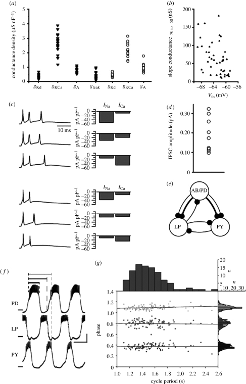
The neuronal networks primarily discussed in this article are the well-characterized circuits composed of a small number of identified neurons that are mostly found in invertebrates. Here, the term ‘identified neuron’ refers to a neuron that exists in a small number of copies, often a single copy, in every animal of a species, has the same overall morphology, synaptic connectivity and axonal projection pattern, produces the same type of electrical activity and has the same behavioural function in every animal. Most notably, the network of identified neurons most frequently referred to in this article is the pyloric circuit in the stomatogastric ganglion of lobsters and crabs, a central pattern-generating circuit that produces a triphasic burst pattern involved in digestion in crustaceans (see figure 1e,f for a schematic of the pyloric circuit and a recording of the rhythmic motor pattern it generates).

Figure 1.

(a–d) Network parameters and (f,g) output measures are variable. (a) Conductance densities of ionic membrane currents in crab inferior cardiac (triangles) and pyloric dilator neurons (circles). Each data point represents one animal. Adapted from Golowasch et al. (1999) and Goldman et al. (2000). (b) Conductance amplitude and activation threshold variability of a potassium current in guinea pig ventral cochlear nucleus neurons. Slope conductance, defined as the slope of the current–voltage relationship between −70 and −50 mV, is used as a measure of conductance amplitude. Adapted from Rothman & Manis (2003). (c) Action potential bursts and current amplitudes in mouse Purkinje neurons show variable current amplitudes in neurons with similar electrical activity. Adapted from Swensen & Bean (2005). (d) Variability in inhibitory post-synaptic current (IPSC) amplitude at a synapse between identified leech heart interneurons. Each data point represents one animal. Adapted from Marder & Goaillard (2006). (e) Simplified schematic of the crustacean pyloric pattern-generating circuit. AB/PD, anterior burster and pyloric dilator pacemaker kernel; LP, lateral pyloric neuron; PY, pyloric constrictor neuron. Thin lines, fast glutamatergic; thick lines, slow cholinergic. (f) Voltage traces of PD, LP and PY neurons in the pyloric motor pattern. Scale bars, 1 s and 10 mV. Definition of intervals PDon-PDoff (black), PDon-LPoff (dark grey) and PDon-PYoff (light grey) are indicated. (e,f) Adapted from Prinz Bucher et al. (2004). (g) Distributions of cycle period and PDon-PDoff, PDon-LPoff and PDon-PYoff phases in 99 lobster pyloric circuits. Phases are defined as interval duration divided by cycle period. Grey scale assignments are as in (f). Adapted from Bucher et al. (2005).

Although most of this article will focus on such identified neuronal networks, many of the lessons learned from these circuits and their models will probably generalize to other neuronal structures (Prinz 2006; Marder & Bucher 2007).

2. Networks are variable

From the moment experimentalists started measuring the properties of neurons and neuronal networks, it has been clear that these properties are variable. This is not surprising, because neuronal networks are biological systems, and all biological systems show some variability.

What do we mean by the ‘properties’ of neuronal networks, and by ‘variability’ of these properties? As defined here, the properties of neuronal networks (and of any dynamic system) fall into two fundamentally different categories, namely parameters and output measures. The parameters that define a neuronal network are biophysical properties that are approximately constant on the time-scales considered here, and include, for example, maximal conductance densities of ionic channels in the membrane of network neurons, the strengths of specific synapses in the network, and the number and morphology of neurons in the network. In contrast, output measures are descriptors of the electrical network activity produced by these network parameters. Examples of output measures are the spike or burst frequency generated by specific neurons in a network and the temporal relationships between activity features in different neurons. Note that both parameters and measures are different from a third category of network descriptors, the dynamic variables of a network. These are time-varying values such as the membrane potential and intracellular calcium concentration of individual neurons or the activation and inactivation state of individual membrane or synaptic conductances. From the computational modelling perspective, dynamic variables are defined by the fact that each variable's dynamics are governed by a separate differential equation.

The term variability as used in this article primarily refers to animal-to-animal differences in the parameters and output measures of identified neurons and neuronal networks. It is tempting to speculate, however, that some of the same principles and mechanisms of network organization that emerge from animal-to-animal comparisons, as described below, might also apply on a slow time-scale within a given animal.

Figure 1 shows parameter and output measure variability in a variety of neuronal systems, both vertebrate and invertebrate. Interestingly, not all measures of network activity are equally variable between animals. For example, figure 1g shows that while the burst period in pyloric rhythms recorded from different lobster stomatogastric ganglia varies up to 2.5-fold (horizontal spread in figure 1g), the relative phasing of burst onset and offset events within a burst cycle appears to be more narrowly constrained, with ranges of typically a small fraction of the mean phase (vertical spreads in figure 1g). It thus appears that there are some network output characteristics that are more faithfully maintained between animals than others. It is likely that this selective maintenance of specific network output measures reflects their importance for the animal's behaviour.

In addition to genetic differences between individual animals, variability in neuronal network properties is thought to be exacerbated by multiple mechanisms of neuronal and synaptic plasticity that are at work in neuronal networks. These mechanisms are engaged differently during the development and lifetime of each individual animal depending on its life history and the changing environments it encountered.

3. Dealing with network variability

Parameter and output measure variability complicate the study of neuronal circuits and of the mechanisms through which they generate electrical activity patterns, because these mechanisms can differ between different versions of an identifiable network in different animals. For example, in half-centre oscillators consisting of two mutually inhibitory neurons, shifting the activation voltage thresholds of the inhibitory synapses to depolarized values decreases the network oscillation period when the component neurons contain little hyperpolarization-activated membrane conductance g(I_h), but has the opposite effect—an increase in network period—when there is a lot of g(I_h) present in the neurons (Sharp et al. 1996). The effect of a parameter change on network activity thus can heavily depend on the values of other network parameters. When, then, can we say that we have truly understood how a network operates?

One obvious answer is that we have understood how an identifiable network operates if we understand the role of all its parameters in all physiologically plausible versions of that network. However, accomplishing this would require that we are able to measure and vary many, if not all, network parameters in the same network instantiation (i.e. the same animal), and do so in multiple animals to sample multiple different network versions. This currently is, and will probably always remain, far beyond what is experimentally feasible.

Constructing and analysing computational network models provides an increasingly appreciated solution to many of these problems. For example, once a computer model of a network is available, it allows the researcher to freely vary all parameters of the network (usually one or a few at a time), including many parameters that are not experimentally accessible, and observe the resulting changes in network output. However, construction of a ‘canonical’ network model whose parameters can then be varied is obviously itself marred by parameter variability and our inability to measure all network parameters simultaneously: what parameter values are one to choose when constructing such a model network?

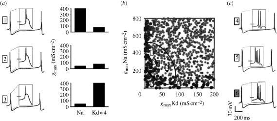
An obvious and ubiquitous approach for dealing with experimental parameter variability when choosing parameter values for a canonical network model is to measure the same parameter, for example, the strength of a given synapse, in multiple animals and use the mean of the resulting distribution of values in the model. Unfortunately, decades of collective experience with model neuron and network construction show that a model constructed with mean parameter values obtained in this manner more often than not fails to generate biologically realistic activity, let alone the activity observed in the biological circuits from which its parameter values were derived. This somewhat discouraging finding is explained by a modelling study (Golowasch et al. 2002) that examines the distribution of neuron models that generate a certain type of activity in the space of the underlying parameter values (figure 2). This and other studies (Goldman et al. 2000; Prinz et al. 2003, 2004; Achard & De Schutter 2006; Taylor et al. 2006, 2009) have shown that such distributions (referred to below as ‘solution spaces’) can have a highly non-convex shape, meaning that the mean of any individual parameter obtained from such a distribution may well fall outside of the distribution itself and thus fail to produce the desired activity when used in a model.

Figure 2.

Failure of parameter averaging for model construction. (a) Voltage traces (left) and sodium and delayed rectifier potassium conductance densities (right) in three versions of a model neuron that generate virtually identical tonic spiking activity with different conductance combinations. Spike shapes are shown in insets. Scale bar from (c) applies. (b) Location of model versions with different electrical activity in the model conductance space. Spiking models with electrical activity as in (a) are indicated by large dark dots. Lighter, smaller dots indicate models that generate bursts of spikes, as in (c). Locations of models from (a,c) are indicated by numbers. Ellipse shows the 1 standard deviation (s.d.) covariance region around model 6. (c) Voltage traces of models that lie within the covariance ellipse but generate bursting activity different from the tonic spiking shown in (a). Model 6 is the model obtained by averaging the conductances of all tonically spiking models, but generates bursts of three spikes. Adapted from Golowasch et al. (2002).

In addition to this ‘failure of averaging’ problem (Golowasch et al. 2002), modelling approaches have to address the more general question what type and structure of model to use. Neuron models vary from extremely simplified integrate-and-fire models through single-compartment conductance-based models to highly complex multi-compartment models with extensive spatial structure. Similarly, network models can vary widely in the number of neurons in the network and their type, heterogeneity and connectivity pattern. The appropriate choice of model type and structure is tightly connected to the scientific questions the model is intended to address. Because they have been discussed extensively elsewhere (Prinz 2006; Calabrese & Prinz 2009), I will not dwell on these more general questions related to neuron and network modelling here, but will instead continue to focus on the particular issues raised by parameter and output measure variability.

4. Embracing variability through ensemble modelling

Rather than struggling or coping with parameter and output measure variability, several recent approaches (Foster et al. 1993; Goldman et al. 2000; Golowasch et al. 2002; Prinz et al. 2003, 2004; Achard & De Schutter 2006; Prinz 2007a,b; Gunay et al. 2008) have sought to embrace variability through what I propose to call ‘ensemble modelling’, in analogy to the usage of the term in systems biology for the modelling of groups of metabolic networks with different underlying kinetics, but similar steady state (Tran et al. 2008). Rather than seeking to construct a single, canonical model neuron or network to replicate the activity of a single, ‘typical’ member of a neuron class, ensemble modelling incorporates variability of the network parameters, the network output measures or both.

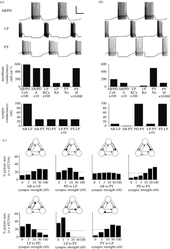
To allow for variability of output measures, ensemble modelling approaches typically define acceptable ranges—based on experimentally observed ranges—for network activity characteristics such as burst period and durations, spike or burst shapes and others. Any model parameter combination that produces model activity within these target ranges is then deemed a suitable model and considered part of a subset of the model's parameter space that is called its ‘solution space’. This is in contrast to more traditional modelling approaches in which, rather than defining a solution space containing multiple parameter sets that generate acceptable network activity, the aim is to identify a unique, optimal parameter set that best reproduces the detailed activity pattern of a single experimental recording. Figure 3a,b shows two examples of pyloric network model versions that are part of a solution space defined by ranges of allowable output measures such as period, burst durations and phase relationships between burst onset and offset events in a burst cycle. The underlying cellular and synaptic parameters of the two networks are clearly different, indicating that similar and physiologically functional network activity can indeed arise from widely varying parameter sets (Prinz et al. 2004), consistent with the biological variability shown in figure 1.

Figure 3.

Parameter variability in model solution spaces. (a,b) Electrical activity (top) and cellular and synaptic parameters (bottom) of two pyloric network models that generate similar and functional activity on the basis of widely different parameters. (c) Distributions of the pyloric network model's solution space over the strengths of the synapses in the circuit. Adapted from Prinz et al. (2004).

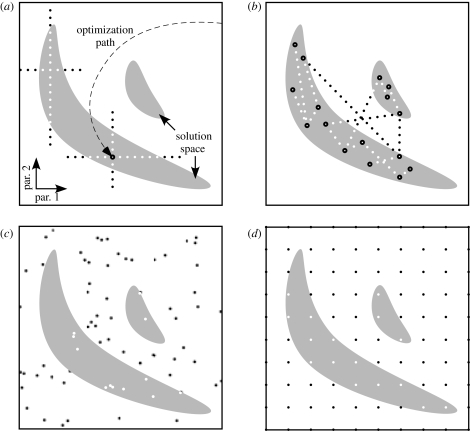
To incorporate network parameter variability, ensemble modelling approaches can use a variety of strategies to identify suitable parameter sets and explore a model network's solution space. Some of these strategies for solution space mapping are schematically represented in figure 4. Solution space exploration can start from a small number of individual solutions obtained through informed hand-tuning of a model or through a model optimization method such as gradient descent or an evolutionary algorithm. From such ‘anchor points’, solution space can then be explored by varying individual parameters one at a time (figure 4a) or interpolating between known solutions (figure 4b). Alternatively, the entire parameter space of a model neuron or network can be covered with a random (figure 4c) or a regular (figure 4d) set of simulation points to explore the extent and shape of solution space. Advantages, disadvantages and technical details of these different approaches to solution space mapping are discussed in more depth elsewhere (Prinz 2007a,b; Calabrese & Prinz 2009).

Figure 4.

Mapping solution spaces. White boxes: schematic representation of parameter space. Grey areas: solution regions. Dots: simulated parameter sets identified as solutions (white) or non-solutions (black) or found as solutions through optimization methods (white centre, black surround). (a) How sensitively model behaviour depends on model parameters can be explored by varying one parameter at a time, starting from a known solution, for example, one identified by an optimization method. (b) After running evolutionary algorithms several times with different results, solution space can be mapped by exploring hyperplanes spanned by subsets of results (lines in this two-dimensional schematic). (c) Stochastic parameter space exploration. (d) Systematic parameter space exploration on a grid. Adapted from Calabrese & Prinz (2009).

5. Structure of neuron and network solution spaces

Ensemble modelling approaches of various flavours have shown that solution spaces of model neurons and networks can extend quite far along the axes of individual model parameters. For example, figure 3c shows that pyloric network models that generate electrical activity within physiologically realistic bounds cover several orders of magnitude for the strengths of all but one of the underlying inhibitory synapses (Prinz et al. 2004). Analysis approaches aimed at the question of whether model solution spaces are contiguous in parameter space have furthermore shown that solutions tend to be part of a connected subspace of the model's whole parameter space (Prinz et al. 2003; Taylor et al. 2006, 2009), although the topological structure of a complex model's solution space can itself be quite complex (Achard & De Schutter 2006) and non-convex (Golowasch et al. 2002), as shown in figure 2.

Because of the high-dimensional nature of parameter and solution spaces of all but the simplest neuronal systems, understanding the internal structure of a model's solution space beyond its extent in one or two dimensions is difficult. However, in the case of regular datasets obtained from systematic exploration of neuronal parameter spaces as pictured in figure 4d, some insight into solution space structure can be gained from a recently developed visualization method called ‘dimensional stacking’ (Taylor et al. 2006). Dimensional stacking allows for a two-dimensional representation of a high-dimensional model parameter space without collapsing or averaging along additional dimensions by representing each entry in a high-dimensional dataset as a pixel whose location in the two-dimensional ‘stack’ is determined by its location in parameter space in a systematic fashion. Such dimensional stacks have yielded insights into the structure of neuronal solution spaces, most notably the finding that these solution spaces tend to show smooth variations of output pleasures such as burst period over wide ranges of parameter space.

The fact that solution spaces tend to be contiguous and often organized in a regular fashion is good news both from the modelling perspective and from the viewpoint of neuronal network stability and robustness. Both for the modeller and for the neuronal system itself, interconnected and smoothly varying solutions mean that small variations in any given parameter—unless they occur in a direction that takes the system out of its solution space—are likely only to change network activity quantitatively without qualitatively disrupting proper network function.

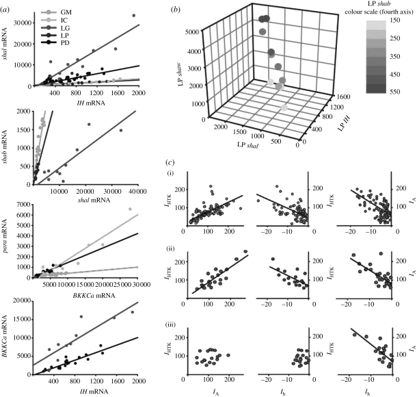
Further information about the internal structure of neuron and network solution spaces comes from recent experimental and modelling evidence which indicates that parameters within a solution space often show pairwise or higher linear relationships. Figure 5 shows such pairwise and four-way correlations from electrophysiology studies (figure 5c) and mRNA copy number measurements (figure 5a,b) in stomatogastric neurons (Schulz et al. 2006, 2007; Khorkova & Golowasch 2007). Such correlations appear to be cell-type specific, suggesting that the functional identity of a given neuron type may reside in the set of parameter correlation rules it maintains rather than in the value of any particular parameter. Although the overall structure of high-dimensional neuron and network solution spaces remains difficult to understand, correlations of the kind shown in figure 5 impose substantial constraints on the possible solution space topologies.

Figure 5.

Conductance correlations in identified neurons. (a) Linear relationships between mRNA copy numbers of pairs of ion channel types in different cell types of the stomatogastric ganglion. GM, gastric mill neuron; IC, inferior cardiac neuron; LG, lateral gastric neuron. Ionic current types corresponding to the different mRNAs are: shal, transient potassium current I_A; IH, hyperpolarization-activated inward current I_h; shab, delayed rectifier potassium current I_Kd; para, sodium current I_Na; BKKCa, calcium-dependent potassium current I_KCa. (b) The LP neuron shows a four-way correlation between shaw, shal, shab and IH mRNA copy numbers. (a,b) Adapted from Schulz et al. (2007). (c) Correlations between current densities (in nA nF⁻¹) in crab PD neurons under different modulatory conditions (decentralized versus non-decentralized): (i) non-decentralized (day 0), (ii) non-decentralized (day 4) and (iii) decentralized (day 4 after decentralization). I_HTK is a high-threshold potassium current. Adapted from Khorkova & Golowasch (2007).

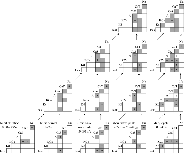
In addition to the experimental evidence for parameter correlations within neuronal solution spaces, such correlations are also found in model solution spaces obtained by parameter space exploration and subsequent selection of biologically realistic model versions (Smolinski & Prinz 2009; Taylor et al. 2009; Hudson & Prinz submitted). Figure 6 shows examples of such conductance correlations in ensembles of bursting model neurons selected for various output measure ranges. In contrast to the experimentally observed conductance correlations shown in figure 5, which are always positive correlations, the modelling results in figure 6 also include negative pairwise conductance correlations, i.e. instances where one conductance decreases when the other increases. It is not currently clear why such negative relationships have not yet been observed in experiments, as they appear to make both functional sense and are feasible within the existing structures of molecular pathways and expression regulation within biological neurons.

Figure 6.

Conductance correlations in model solution spaces. Each triangular panel shows pairwise conductance correlations found in a subset of model neurons from a model neuron set constructed by systematic parameter space exploration (Prinz et al. 2003). Membrane conductances include a sodium conductance (Na), transient and slow calcium conductances (CaT and CaS), transient, delayed rectifier and calcium-dependent potassium conductances (A, Kd and KCa) and a leak conductance. ‘Parent’ populations (bottom row) contain bursting model neurons that match one output measure range, as indicated. Slow wave refers to the slow voltage oscillation underlying the spikes. Duty cycle is defined as the ratio between burst duration and burst period. ‘Child’ populations (upper rows) are obtained by combining their parents' output measure ranges as indicated by arrows. Within each triangular panel, ‘plus ’ indicates a positive pairwise conductance correlation, ‘minus’ indicates a negative pairwise conductance correlation and grey shading indicates that a pairwise correlation was present in one of the parents. Adapted from Hudson & Prinz (submitted).

A further conclusion from the modelling results presented in figure 6 is that the effects of applying multiple output measure constraints on the shape and structure of model solution spaces are anything but simple, and often highly counterintuitive. For example, bursting model neurons with burst durations between 0.5 and 0.75 s (lower left corner in figure 6) show positive correlations between the Na and CaT conductances and the CaS and KCa conductances, and a negative correlation between the CaT and KCa conductances, while bursting models with burst periods between 1 and 2 s (second from left in bottom row of figure 6) show positive correlations between CaS and A and CaS and leak conductances, and a negative correlation between the CaT and CaS conductances. But when combined, the burst duration and burst period selection criteria define a model population (leftmost panel in second row from bottom) in which only the conductance correlations related to burst duration persist, whereas those related to burst period are no longer present. Conversely, combining selection criteria can also lead to the appearance of new conductance correlations in the child population that were present in neither of the parent populations. One such example is the positive correlation between the A and CaT conductances found in bursting models with a slow wave peak between −55 and −25 mV and a duty cycle between 0.3 and 0.4 (rightmost panel in second row from bottom) that is not present if only slow wave peak or only duty cycle are constrained.

6. Summary

Both the cellular and synaptic parameters of neuronal networks and their output measures can be highly variable. This poses substantial problems for efforts at accurate computational modelling of neuronal systems, because network parameters can not usually all be measured in the same individual and averaging over data from multiple individuals to construct a canonical network model that represents all networks of a given type is destined to fail in most cases.

Ensemble modelling represents a relatively recent approach that not only overcomes most of these problems, but also reproduces and studies biological variability rather than ignoring it. With increasing computational power available to neuroscience researchers, it stands to reason that ensemble modelling approaches will continue and perhaps expand the fruitful interplay between experimentation and computational modelling that allows us to study signal processing in neuronal circuits with all available tools.

References

- Achard P., De Schutter E.2006Complex parameter landscape for a complex neuron model. PLoS Comput. Biol. 2, 794–804 [DOI] [PMC free article] [PubMed] [Google Scholar]
- Bucher D., Prinz A. A., Marder E.2005Animal-to-animal variability in motor pattern production in adults and during growth. J. Neurosci. 25, 1611–1619 (doi:10.1523/JNEUROSCI.3679-04.2005) [DOI] [PMC free article] [PubMed] [Google Scholar]
- Calabrese R. L., Prinz A. A.2009Realistic modeling of small neuronal networks. In Computational modeling methods for neuroscientists (ed. Schutter E. D.). Cambridge, MA: MIT Press [Google Scholar]
- Foster W. R., Ungar L. H., Schwaber J. S.1993Significance of conductances in Hodgkin–Huxley models. J. Neurophysiol. 70, 2502–2518 [DOI] [PubMed] [Google Scholar]
- Goldman M. S., Golowasch J., Abbott L. F., Marder E.2000Dependence of firing pattern on intrinsic ionic conductances: sensitive and insensitive combinations. Neurocomputing 32, 141–146 [Google Scholar]
- Golowasch J., Abbott L. F., Marder E.1999Activity-dependent regulation of potassium currents in an identified neuron of the stomatogastric ganglion of the crab Cancer borealis. J. Neurosci. 19, 33 [DOI] [PMC free article] [PubMed] [Google Scholar]
- Golowasch J., Goldman M. S., Abbott L. F., Marder E.2002Failure of averaging in the construction of a conductance-based neuron model. J. Neurophysiol. 87, 1129–1131 [DOI] [PubMed] [Google Scholar]
- Gunay C., Edgerton J. R., Jaeger D.2008Channel density distributions explain spiking variability in the globus pallidus: a combined physiology and computer simulation database approach. J. Neurosci. 28, 7476–7491 (doi:10.1523/JNEUROSCI.4198-07.2008) [DOI] [PMC free article] [PubMed] [Google Scholar]
- Hudson A. E., Prinz A. A.Submitted Conductance ratios and cellular identity. PLoS Comput. Biol. [DOI] [PMC free article] [PubMed] [Google Scholar]
- Khorkova O., Golowasch J.2007Neuromodulators, not activity, control coordinated expression of ionic currents. J. Neurosci. 27, 8709–8718 (doi:10.1523/JNEUROSCI.1274-07.2007) [DOI] [PMC free article] [PubMed] [Google Scholar]
- Marder E., Bucher D.2007Understanding circuit dynamics using the stomatogastric nervous system of lobsters and crabs. Annu. Rev. Physiol. 69, 291–316 (doi:10.1146/annurev.physiol.69.031905.161516) [DOI] [PubMed] [Google Scholar]
- Marder E., Goaillard J. M.2006Variability, compensation and homeostasis in neuron and network function. Nat. Rev. Neurosci. 7, 563–574 (doi:10.1038/nrn1949) [DOI] [PubMed] [Google Scholar]
- Prinz A. A.2006Insights from models of rhythmic motor systems. Curr. Opin. Neurobiol. 16, 615–620 (doi:10.1016/j.conb.2006.10.001) [DOI] [PubMed] [Google Scholar]
- Prinz A. A.2007aComputational exploration of neuron and neuronal network models in neurobiology. In Methods in molecular biology: bioinformatics (ed. Crasto C.). Totowa, NJ: Humana Press; [DOI] [PubMed] [Google Scholar]
- Prinz A. A.2007bNeuronal parameter optimization. Scholarpedia 2, 1903 (doi:10.4249/scholarpedia.1903) [Google Scholar]
- Prinz A. A., Billimoria C. P., Marder E.2003Alternative to hand-tuning conductance-based models: construction and analysis of databases of model neurons. J. Neurophysiol. 90, 3998–4015 (doi:10.1152/jn.00641.2003) [DOI] [PubMed] [Google Scholar]
- Prinz A. A., Bucher D., Marder E.2004Similar network activity from disparate circuit parameters. Nat. Neurosci. 7, 1345–1352 (doi:10.1038/nn1352) [DOI] [PubMed] [Google Scholar]
- Rothman J. S., Manis P. B.2003Differential expression of three distinct potassium currents in the ventral cochlear nucleus. J. Neurophysiol. 89, 3070–3082 (doi:10.1152/jn.00125.2002) [DOI] [PubMed] [Google Scholar]
- Schulz D. J., Goaillard J. M., Marder E.2006Variable channel expression in identified single and electrically coupled neurons in different animals. Nat. Neurosci. 9, 356–362 (doi:10.1038/nn1639) [DOI] [PubMed] [Google Scholar]
- Schulz D. J., Goaillard J. M., Marder E.2007Quantitative expression profiling of identified neurons reveals cell-specific constraints on highly variable levels of gene expression. Proc. Natl Acad. Sci. USA 104, 13 187–13 191 (doi:10.1073/pnas.0705827104) [DOI] [PMC free article] [PubMed] [Google Scholar]
- Sharp A. A., Skinner F. K., Marder E.1996Mechanisms of oscillation in dynamic clamp constructed two-cell half-center circuits. J. Neurophysiol. 76, 867–883 [DOI] [PubMed] [Google Scholar]
- Smolinski T. G., Prinz A. A.2009Computational intelligence in modeling of biological neurons: a case study of an invertebrate pacemaker neuron. In Int. Joint Conf. on Neural Networks, Atlanta, GA, pp. 2964–2970 [Google Scholar]
- Swensen A. M., Bean B. P.2005Robustness of burst firing in dissociated Purkinje neurons with acute or long-term reductions in sodium conductance. J. Neurosci. 25, 3509–3520 (doi:10.1523/JNEUROSCI.3929-04.2005) [DOI] [PMC free article] [PubMed] [Google Scholar]
- Taylor A. L., Hickey T. J., Prinz A. A., Marder E.2006Structure and visualization of high-dimensional conductance spaces. J. Neurophysiol. 96, 891–905 (doi:10.1152/jn.00367.2006) [DOI] [PubMed] [Google Scholar]
- Taylor A. L., Goaillard J. M., Marder E.2009How multiple conductances determine electrophysiological properties in a multicompartment model. J. Neurosci. 29, 5573–5586 (doi:10.1523/JNEUROSCI.4438-08.2009) [DOI] [PMC free article] [PubMed] [Google Scholar]
- Tran L. M., Rizk M. L., Liao J.2008Ensemble modeling of metabolic networks. Biophys. J. 95, 5606–5617 (doi:10.1529/biophysj.108.135442) [DOI] [PMC free article] [PubMed] [Google Scholar]