DDSolver: An Add-In Program for Modeling and Comparison of Drug Dissolution Profiles

Abstract

In recent years, several mathematical models have been developed for analysis of drug dissolution data, and many different mathematical approaches have been proposed to assess the similarity between two drug dissolution profiles. However, until now, no computer program has been reported for simplifying the calculations involved in the modeling and comparison of dissolution profiles. The purposes of this article are: (1) to describe the development of a software program, called DDSolver, for facilitating the assessment of similarity between drug dissolution data; (2) to establish a model library for fitting dissolution data using a nonlinear optimization method; and (3) to provide a brief review of available approaches for comparing drug dissolution profiles. DDSolver is a freely available program which is capable of performing most existing techniques for comparing drug release data, including exploratory data analysis, univariate ANOVA, ratio test procedures, the difference factor f₁, the similarity factor f₂, the Rescigno indices, the 90% confidence interval (CI) of difference method, the multivariate statistical distance method, the model-dependent method, the bootstrap f₂ method, and Chow and Ki’s time series method. Sample runs of the program demonstrated that the results were satisfactory, and DDSolver could be served as a useful tool for dissolution data analysis.

Electronic supplementary material

The online version of this article (doi:10.1208/s12248-010-9185-1) contains supplementary material, which is available to authorized users.

INTRODUCTION

In vitro dissolution testing plays an important role in drug formulation development and quality control. It can be used not only as a primary tool to monitor the consistency and stability of drug products but also as a relatively rapid and inexpensive technique to predict in vivo absorption of a drug formulation. Therefore, quantitative evaluation of drug dissolution characteristics is of great interest to pharmaceutical scientists.

A wide variety of mathematical models have been developed to fit the drug release data, most of which are presented as nonlinear equations. Because there is no available computer program for fitting drug release data using these specific nonlinear equations, it is desirable to develop a nonlinear fitting program for solving these problems in a convenient way. However, until now, only one special program has been reported for fitting dissolution data, and only five release models have been implemented, and these could be applied only over a limited range (1). Alternatively, the nonlinear fitting of dissolution data can be performed using other professional statistical software packages such as MicroMath Scientist (2), GraphPad Prism (3), SigmaPlot (4), or SYSTAT (5). However, these programs require the user to define the equation manually and to provide an initial value for each parameter. This may make it difficult for new users to implement the procedure. Therefore, it is necessary to investigate an easy-to-use program for fitting release data with more ready-to-use dissolution models.

Another important area in dissolution data analysis is assessment of the similarity between dissolution profiles. Several approaches have been developed for comparing dissolution profiles, including approaches using the difference factor f₁ and the similarity factor f₂ (6), the Rescigno indices approaches (7), ratio-test approaches (8), ANOVA-based approaches (9), multivariate statistical approaches (10), and model-dependent approaches (11). It can be seen that the mathematical theory in this field has been well developed for more than 10 years. However, to the authors’ knowledge, no computer software package has been developed to facilitate calculations in this field; therefore, data analysis can be done only by hand or be partially done by professional statistical programs. This is time-consuming, and transcription errors are a common problem. Therefore, it is worthwhile to explore a program to streamline these tasks.

This paper presents a versatile and freely available add-in program, called DDSolver, which can be used (1) to facilitate the modeling of dissolution data using nonlinear optimization methods based on a built-in model library containing forty dissolution models, (2) to simplify the task of assessing the similarity between dissolution profiles using various popular approaches, and (3) to speed up the calculation, reduce user errors, and provide a convenient way to report dissolution data quickly and easily. The aim of this article is to report on the development of the specialized program for analysis of dissolution data.

MATERIALS AND METHODS

Interface

DDSolver is a menu-driven add-in program for Microsoft Excel written in Visual Basic for Applications. Calculation using Excel offers a number of advantages over other software packages, the most attractive of which is ease of use. Most scientists are already familiar with Excel because of its wide availability and high flexibility. As shown in Fig. 1, after the program has been installed, a pull-down menu called DDSolver will appear on the menu bar when Excel is launched. Users can choose any module by clicking on the item in the pull-down menu and can input dissolution data by simple drag selection of the corresponding range of cells in the spreadsheet, as shown in Fig. 2. DDSolver provides a range of customizable options for each module, such as convergence and maximum number of iterations of the nonlinear optimization algorithm, initial parameter estimates, number of decimal places in the calculated results, chart output, and Microsoft Word report generation. In addition, a built-in sample dataset can be loaded by clicking on the sample button in each module. This is provided as a guide for new users to help them arrange their data into a suitable form for processing by the program.

Fig. 1.

Interface of the DDSolver program. After the program is installed, a pull-down menu will appear in the menu bar when Excel is launched

Fig. 2.

Interface of the DDSolver program. Dissolution data can be entered by drag-selecting the corresponding range of cells in the spreadsheet

Drug Dissolution Models

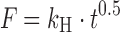
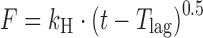
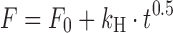
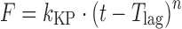
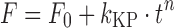
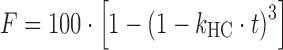
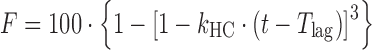
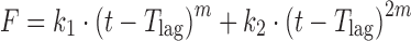
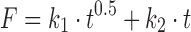
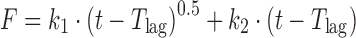
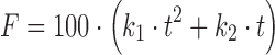
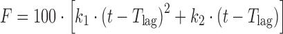
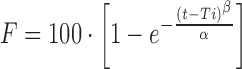
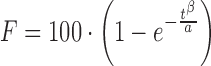
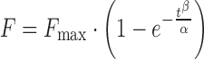
Since the development of the Higuchi equation in 1961 (12), numerous mathematical models have been proposed for quantitative evaluation of in vitro drug release behavior. This work was not performed to assess any particular model or to discuss the statistical or mechanical meaning of each model parameter, because these topics have been well reviewed previously (13,14). In fact, this work was intended to establish a model library and to assemble it into a ready-to-use module which can be easily accessed through the DDSolver program. For this purpose, a wide range of dissolution models was collected. Table I summarizes all the models implemented in the program; in all cases, F is the percentage of drug released at time t. Once the model library has been established, the release data can be easily fitted to any available model followed by quick generation of scatter plots with fitted curves for each individual dataset and a scatter plot with error bars and fitted curves for average data.

Table I.

Models Available in DDSolver for Fitting Drug Release Data^a

Module	Model	Equation	Parameter(s)	Reference(s)
# 301b	Zero-order		k 0	(15)
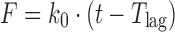
# 302b, c	Zero-order with Tlag		k 0, T lag	(16)
# 303b, d	Zero-order with F0		k 0, F 0	(13)
# 304e	First-order		k 1	(8)
# 305c, e	First-order with T lag		k 1, T lag	(17)
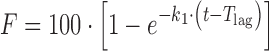
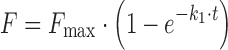
# 306e, f	First-order with F max		k 1, F max	(18)
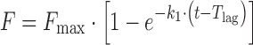
# 307c, e, f	First-order with T lag and F max		k 1, T lag, F max	(19)
# 308g	Higuchi		k H	(12)
# 309c, g	Higuchi with T lag		k H, T lag	(20)
# 310d, g	Higuchi with F 0		k H, F 0	(21)
# 311h	Korsmeyer–Peppas		k KP, n	(22,23)
# 312c, h	Korsmeyer–Peppas with T lag		k KP, n, T lag	(20)
# 313d, h	Korsmeyer–Peppas with F 0		k KP, n, F 0	(13)
# 314i	Hixson–Crowell		k HC	(24)
# 315c, i	Hixson–Crowell with T lag		k HC, T lag	(25)
# 316j	Hopfenberg		k HB, n	(26)
# 317c, j	Hopfenberg with T lag		k HB, n, T lag	(27)
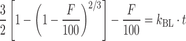
# 318k	Baker–Lonsdale		k BL	(28)
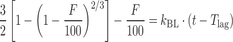
# 319c, k	Baker–Lonsdale with T lag		k BL, T lag	(28)
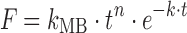
# 320l	Makoid–Banakar		k MB, n, k	(29)
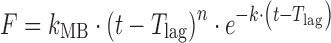
# 321c, l	Makoid–Banakar with T lag		k MB, n, k, T lag	(29)
# 322m	Peppas–Sahlin_1		k 1, k 2, m	(30)
# 323c, m	Peppas–Sahlin_1 with T lag		k 1, k 2, m, T lag	(21)
# 324n	Peppas–Sahlin_2		k 1, k 2	(30)
# 325c, n	Peppas–Sahlin_2 with T lag		k 1, k 2, T lag	(30)
# 326o	Quadratic		k 1, k 2	(8,13)
# 327c, o	Quadratic with T lag		k 1, k 2, T lag	(8)
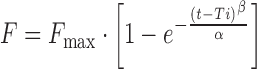
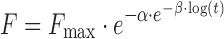
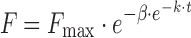
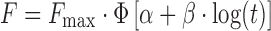
# 328p, q	Weibull_1		α, β, Ti	(31)
# 329p	Weibull_2		α, β	(11)
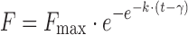
# 330f, p	Weibull_3		α, β, F max	(18)
# 331f, p, q	Weibull_4		α, β, Ti, F max	(32)
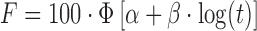
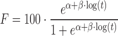
# 332r	Logistic_1		α, β	(11)
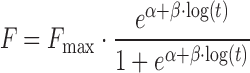
# 333f, r	Logistic_2		α, β, F max	(18,33)
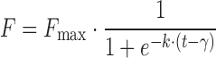
# 334f, s	Logistic_3		k, γ, F max	(8,32)
# 335t	Gompertz_1		α, β	(18)
# 336f, t	Gompertz_2		α, β, F max	(18,19)
# 337f, u	Gompertz_3		k, γ, F max	(8,32)
# 338f, v	Gompertz_4		k, β, F max	(34)
# 339w	Probit_1		α, β	(11,18)
# 340f, w	Probit_2		α, β, F max	(18)

^aIn all models, F is the fraction(%) of drug released in time t

^b k ₀ is the zero-order release constant

^c T _lag is the lag time prior to drug release

^d F ₀ is the initial fraction of the drug in the solution resulting from a burst release

^e k ₁ is the first-order release constant

^f F _max is the maximum fraction of the drug released at infinite time

^g k _H is the Higuchi release constant

^h k _KP is the release constant incorporating structural and geometric characteristics of the drug-dosage form; n is the diffusional exponent indicating the drug-release mechanism

ⁱ k _HC is the release constant in Hixson–Crowell model

^j k _HB is the combined constant in Hopfenberg model, k _HB = k ₀/(C ₀ × a ₀), where k ₀ is the erosion rate constant, C ₀ is the initial concentration of drug in the matrix, and a ₀ is the initial radius for a sphere or cylinder or the half thickness for a slab; n is 1, 2, and 3 for a slab, cylinder, and sphere, respectively

^k k _BL is the combined constant in Baker–Lonsdale model, k _BL = [3 × D × Cs/(r ²₀ × C ₀)], where D is the diffusion coefficient, Cs is the saturation solubility, r ₀ is the initial radius for a sphere or cylinder or the half-thickness for a slab, and C ₀ is the initial drug loading in the matrix

^l k _MB, n, and k are empirical parameters in Makoid–Banakar model (k _MB, n, k > 0)

^m k ₁ is the constant related to the Fickian kinetics; k ₂ is the constant related to Case-II relaxation kinetics; m is the diffusional exponent for a device of any geometric shape which inhibits controlled release

ⁿ k ₁ is the constant denoting the relative contribution of t ^0.5-dependent drug diffusion to drug release; k ₂ is the constant denoting the relative contribution of t-dependent polymer relaxation to drug release

^o k ₁ is the constant in Quadratic model denoting the relative contribution of t ²-dependent drug release; k ₂ is the constant in Quadratic model denoting the relative contribution of t-dependent drug release

^p α is the scale parameter which defines the time scale of the process; β is the shape parameter which characterizes the curve as either exponential (β = 1; case 1), sigmoid, S-shaped, with upward curvature followed by a turning point (β > 1; case 2), or parabolic, with a higher initial slope and after that consistent with the exponential (β < 1; case 3)

^q Ti is the location parameter which represents the lag time before the onset of the dissolution or release process and in most cases will be near zero

^r α is the scale factor in Logistic 1 and 2 models; β is the shape factor in Logistic 1 and 2 models

^s k is the shape factor in Logistic 3 model; γ is the time at which F = F _max/2

^t α is the scale factor in Gompertz 1 and 2 models; β is the shape factor in Gompertz 1 and 2 models

^u k is the shape factor in Gompertz 3 model; γ is the time at which F = F _max/exp(1) ≈ 0.368 × F _max

^v β is the scale factor in Gompertz 4 model; k is the shape factor in Gompertz 4 model

^wФ is the standard normal distribution; α is the scale factor in Probit model; β is the shape factor in Probit model

Nonlinear Optimization Algorithm

For fitting dissolution models to non-transformed data, DDSolver uses the nonlinear least-squares curve-fitting technique, which determines the parameter values that minimize the sum of squares (SS) or optionally the weighted sum of squares (WSS):

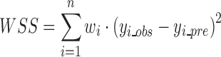where n is the number of observations, w_i is the weighting factor, which can be optionally set as 1, 1/y_{i_obs} or 1/y_{i_obs}² for fitting dissolution data, y_{i_obs} is the ith observed y value, and y_{i_pre} is the ith predicted y value. To minimize the objective function SS or WSS and to find the best parameters, one of the most robust minimization algorithms, the Nelder–Mead simplex algorithm, was used (35). This method is a popular, computationally compact, and often effective method for nonlinear optimization. Compared with the classical Gauss–Newton algorithm or the modified Gauss–Newton algorithm (e.g., Marquardt’s algorithm), which require the linearization of the nonlinear model by taking a Taylor series expansion and which also involve matrix calculations, the simplex method has several advantages: (1) it does not require calculation of derivatives or partial derivatives and therefore can quickly find the best-fit values of the parameters; (2) it is less sensitive than other methods to a poor choice of initial estimates and rarely converges to a local minimum; and (3) it can be used with discontinuous functions (36). One of the disadvantages of the Nelder–Mead algorithm is that it can be very expensive and/or time-consuming for problems with objective functions that are severely elongated or when the number of the variables becomes large. Since most of the dissolution equations only have no more than four parameters and do not suffer severely from this problem, it appears to be suited for application in this situation.

Initial Parameters

An initial value for each parameter in the equation must be provided before performing the iterative optimization. A good guess for the initial values will result in fast convergence and markedly reduce the possibility of falling into a local minimum. DDSolver provides a number of methods for obtaining appropriate initial values, including simple linear regression, multiple linear regression, trial and error, the empirical method, and various combinations of these. For model equations that can be rearranged into a linear form, the simple linear regression method is preferred. It is an effective way to obtain appropriate initial values for most dissolution models. Take the first-order model, for example; its equation is 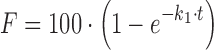, which can be rearranged into the form , from which an initial value of k₁ can be easily estimated by fitting a linear equation with intercept zero to the transformed data.

However, in cases where linear transformation of the model equation produces multiple line segments, the multiple linear regression method should be used. The Makoid–Banakar model with a rearranged model equation, , is a case of this type. The trial-and-error method is used for assessing the initial values of parameters when the Hopfenberg model is used, whose model equation is 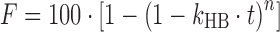, which cannot be linearized before the parameter n is determined. In this case, DDSolver will use n = 1 and a corresponding value of k_HB which is subsequently estimated by simple linear regression during the first trial to obtain a value of WSS. Then, n = 2 and n = 3 will be used for the second and the third trials, with the pair of n and k_HB values which produces the smallest value of WSS serving as the most appropriate initial values.

The empirical method is another effective way for obtaining initial values when the model equation cannot be linearly transformed. For example, when the Peppas–Sahlin model with equation 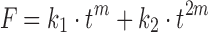is used, DDSolver will suggest an empirical value of 0.45 as the initial value of m, because m lies within the range from 0 to 1 in most cases. Besides the methods mentioned above, DDSolver also allows the user to specify an initial value for each parameter manually.

Model Selection Criteria

The selection of a suitable model for fitting dissolution data is essential, not only for quantitative evaluation of drug release characteristics but also for comparison of dissolution profiles using model-dependent approaches. DDSolver provides a number of statistical criteria for evaluating the goodness of fit of a model, including the correlation coefficient (R_obs–pre), the coefficient of determination (Rsqr, R², or COD), the adjusted coefficient of determination (Rsqr_adj or R²_adjusted), the mean square error (MSE), the standard deviation of the residuals (MSE_root or Sy.x), SS, WSS, the Akaike Information Criterion (AIC), and the Model Selection Criterion (MSC). Among these criteria, the most popular ones in the field of dissolution model identification are the R²_adjusted, the AIC (37), and the MSC (38).

For release models with the same number of parameters, the coefficient of determination (R²) can be used to discriminate the most appropriate model. However, when comparing models with different numbers of parameters, the adjusted coefficient of determination should be used:

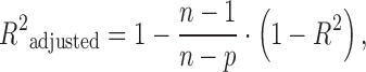where n is the number of data points and p is the number of parameters in the model. This is because R² will always increase as more parameters are included, whereas R²_adjusted may decrease when over-fitting has occurred. Therefore, the best model should be the one with the highest R²_adjusted, rather than that with the highest R² (13).

The Akaike Information Criterion has been used for selecting optimal models for more than 35 years (37). Its general applicability and simplicity make it an excellent and popular criterion for various purposes, including drug dissolution data analysis (33). The AIC as defined below is dependent on the magnitude of the data as well as the number of data points:

where n is the number of data points, WSS is the weighted sum of squares, and p is the number of parameters in the model. When comparing two models with different numbers of parameters, the model with a lower AIC value can be considered to be the better model, but how much lower the value needs to be to make the difference between the models statistically significant cannot be determined because the distribution of the AIC values is unknown. It should be noted that when a comparison is made, the weighting scheme used in each model must be the same.

The MSC provided by MicroMath Corporation (38) is another statistical criterion for model selection which is attracting increasing attention in the field of dissolution data modeling (32,39); it is defined as:

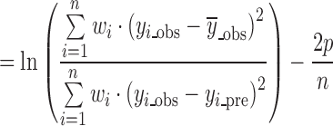where w_i is the weighting factor, which is usually equal to 1 for fitting dissolution data, y_{i_obs} is the ith observed y value, y_{i_pre} is the ith predicted y value, is the mean of all observed y-data points, p is the number of parameters in the model, and n is the number of data points. The MSC is a modified reciprocal form of the AIC and has been normalized so that it is independent of the scaling of the data points. When comparing different models, the most appropriate model will be that with the largest MSC. It is, therefore, quite easy to develop a feeling for what the MSC means in terms of how well the model fits the data. Generally, a MSC value of more than two to three indicates a good fit (40).

Although all the criteria mentioned above can be calculated by DDSolver to assess the goodness of fit of dissolution models, it should be noted that when mechanistic models are evaluated, model selection should be based, not only on the goodness of fit but also on the mechanistic plausibility of the model. More detailed discussions on the difference between mechanism-based models and empirical mathematical models can be found in previous reports (14,41).

Dissolution Profile Comparison

During the past decade, several approaches have been proposed for assessing the similarity between dissolution profiles. As shown in Table II, DDSolver implements most of the widely used methods, especially those recommended by the FDA. To give readers an intimate knowledge of these methods and to provide an explanation of the output results of the program, a brief review of these methods, as well as the advantages and disadvantages of each method, is presented in this section. Due to the limitation on the length of this paper, the contents are provided in the supplementary material to this article.

Table II.

Methods Available in DDSolver for Comparing Drug Dissolution Profiles

Module	Method	Reference(s)
# 401	Exploratory data analysis	(42)
# 402	Univariate ANOVA	(8,9)
# 403	Ratio test procedures	(8,13)
# 404	Difference factor, f 1	(6,43)
# 405	Similarity factor, f 2	(6,43)
# 406	Rescigno index	(7)
# 407	90% CI of difference method	(10)
# 408	Multivariate statistical distance method	(10,43)
# 409	Model-dependent approaches	(11,43)
# 410	Bootstrap f 2 method	(44,45)
# 411	Chow and Ki’s method	(46)

Other Dissolution Functions

One of the distinctive features of DDSolver is the implementation of eight user-defined functions for characterizing drug release curves as shown in Table III and 11 user-defined functions for evaluating the similarity between dissolution profiles as shown in Table IV. All the parameters of these functions are calculated using a model-independent nonparametric method based on the linear trapezoidal rule. These functions can be conveniently used in the same way as SUM() or other built-in functions in Microsoft Excel. Figure 3 shows a sample sheet with a full application of all the dissolution functions. It should be noted that most of the parameters can be alternatively calculated using a model-dependent method (47).

Table III.

Parameters for Characterizing Drug Release Curve

Abbreviation, description	Equation	Function in DDSolver	Reference(s)
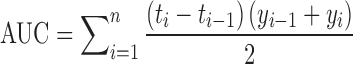
AUC, area under the dissolution curve		DD_AUC	(47)
ABC, area between the drug dissolution curve and its asymptote		DD_ABC	(48,49)
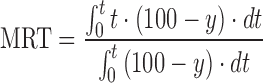
MRT, mean residence time of the drug substance molecules in the dosage form		DD_MRT	(49)
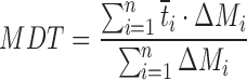
MDT, mean dissolution time		DD_MDT	(50,51)
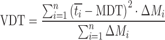
VDT, variance of dissolution time		DD_VDT	(50,51)
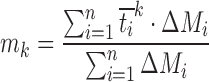
m k, moments of dissolution times of order k		DD_MDTk	(33,50)
RD, relative dispersion of dissolution time, CV2 (coefficient of variation)		DD_RD	(33,51)
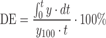
DE, dissolution efficiency		DD_DE	(52)

n number of sampling points; t _i ith time point; y _i percentage of drug dissolved at time t _i; M _last accumulative percentage of drug dissolved at the last time point; y percentage of drug dissolved at time t; time at the midpoint between i and i–1; ∆M _i additional amount of drug dissolved between i and i–1; k order of the moments of dissolution times; y ₁₀₀ maximum percentage of drug dissolved over the time period 0−t

Table IV.

Parameters for Assessing the Difference Between Dissolution Profiles

Abbreviation, description	Equation	Function in DDSolver	Reference(s)
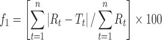
f 1, difference factora		DD_f1	(6)
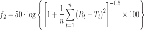
f 2, similarity factora		DD_f2	(6)
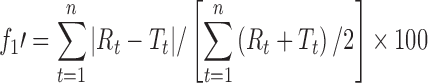
f 1’, difference factor modified by Costa P.a		DD_f1cp	(13)
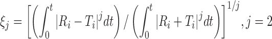
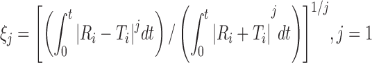
ξ 1, first-order Rescigno indexa, b		DD_res1	(7)
ξ 2, second-order Rescigno indexa, b		DD_res2	(7)
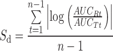
S d, difference in similarityc		DD_Sd	(53)
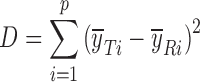
D, sum of squared mean differencesd		DD_D	(44,54)
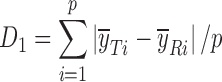
D 1, mean distanced		DD_D1	(55,56)
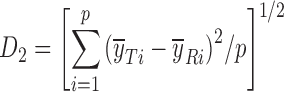
D 2, mean squared distanced		DD_D2	(56)
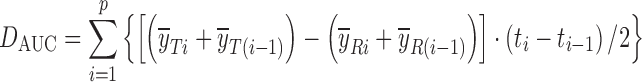
D AUC, difference of area under the profilesd,e		DD_DAUC	(56)
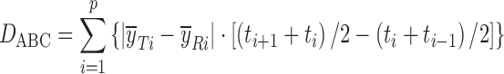
D ABC, area between the profilesd,e		DD_DABC	(56)

^a R _t, T _t are the percentage dissolved of the reference and test profile, respectively, at time point t; n is the number of sampling points

^b j is 1 and 2 for the first- (ξ ₁) and second-order (ξ ₂) Rescigno indexes, respectively

^c n is the number of sampling points; AUC_Rt and AUC_Tt are the areas under the dissolution curves of the reference and test formulations, respectively, at time t

^d p is the number of sampling points; and are the mean dissolution values of the test and reference profiles respectively at the ith time point

^e t _i is the ith sampling time point

Fig. 3.

Sample sheet showing the use of predefined dissolution functions; the names of the functions are listed in Column G, while Column F shows the calculation results

Besides all the methods and parameters mentioned above, many other approaches have been reported for comparing dissolution profiles, such as principal component analysis (18), linear mixed-effects model (57), nonlinear mixed-effects model (58), artificial neural networks with similarity factor (59), partially Bayesian approach (60), and other analogous statistics of the Mann–Whitney statistic, the Kolmogorov–Smirnov “D” statistic and the chi-squared statistic (61).

RESULTS AND DISCUSSION

Validation of a newly developed program is an important aspect of its acceptability. For this purpose, some typical modules of the DDSolver program were evaluated using previously published data. Because of the limitation on the length of this paper, the results have been provided in the supplementary material to this article. Sample runs were performed using one module for dissolution-model fitting using the Weibull model and five modules for comparison of dissolution profiles using f₁, f₂, the Rescigno index ξ₁, the Rescigno index ξ₂, the multivariate-confidence-region method, and Chow and Ki’s time series method.

As summarized in Table V, the results indicated that all the parameters calculated, using DDSolver, were identical to those given in previous reports. It should be noted that slight numerical differences between the estimates of DDSolver and those of previous reports were observed when the Weibull model was used to fit the dissolution data. This might be because different tolerance and convergence settings and optimization strategies were adopted.

Table V.

Results of Sample Runs to Test the Reliability of the Program

Module	Resultsa	Reference
Dissolution data modeling	All the model parameters calculated using DDSolver are nearly identical	(8)
Pairwise procedures	All the f 1 factor, f 2 factor and Rescigno indexes are identical	(8)
Multivariate confidence region	The MSD and its 90% CI and other related statistics are identical	(10)
Chow and Ki’s method	Both the results for global similarity and local similarity are identical	(46)

^aCompared with those given in previous reports

Although DDSolver provides many types of approaches for comparing dissolution profiles, as pointed out by Polli et al. (8), “no one method appears as the best.” In fact, the main objective of the present research is to provide a software tool for facilitating the calculations in dissolution data analysis; more discussions on the advantages and disadvantages of each method can be found in previous review (42).

CONCLUSIONS

The DDSolver program was developed to facilitate the modeling and comparison of drug dissolution data. The program can fit drug release data using nonlinear optimization techniques in an easy-to-use spreadsheet environment. It is the first reported program which is specifically designed to assess the similarity between dissolution profiles. The program is capable of performing most existing techniques for comparing drug release data, including exploratory data analysis, univariate ANOVA, ratio test procedures, the difference factor f₁, the similarity factor f₂, the Rescigno indices, the 90% CI of difference method, the multivariate statistical distance method, the model-dependent method, the bootstrap f₂ method, and Chow and Ki’s time series method. In addition, several user-defined functions for characterizing drug-release curves and for assessing the similarity between dissolution profiles are also implemented in the program. These additional functions can be conveniently used in the same way as the built-in functions in Microsoft Excel. Sample runs of the program demonstrated that DDSolver can be considered a reliable program for dissolution data analysis.

The DDSolver program is freely available. The interested reader can obtain the program from the supplementary material to this article. The program was developed and tested in Microsoft Excel 2003 (both English and Simplified Chinese versions) in a Windows XP SP2 environment and was compatible with Microsoft Excel 2007 and 2010 on Windows platform.

Electronic supplementary material

Below is the link to the electronic supplementary material.

References

- 1.Lu DR, Abu-Izza K, Mao F. Nonlinear data fitting for controlled release devices: an integrated computer program. Int J Pharm. 1996;129:243–51. doi: 10.1016/0378-5173(95)04356-X. [DOI] [Google Scholar]
- 2.Phaechamud T. Variables influencing drug release from layered matrix system comprising hydroxypropyl methylcellulose. AAPS PharmSciTech. 2008;9:668–74. doi: 10.1208/s12249-008-9085-1. [DOI] [PMC free article] [PubMed] [Google Scholar]
- 3.Di Colo G, Baggiani A, Zambito Y, Mollica G, Geppi M, Serafini MF. A new hydrogel for the extended and complete prednisolone release in the GI tract. Int J Pharm. 2006;310:154–61. doi: 10.1016/j.ijpharm.2005.12.002. [DOI] [PubMed] [Google Scholar]
- 4.Papadopoulou V, Kosmidis K, Vlachou M, Macheras P. On the use of the Weibull function for the discernment of drug release mechanisms. Int J Pharm. 2006;309:44–50. doi: 10.1016/j.ijpharm.2005.10.044. [DOI] [PubMed] [Google Scholar]
- 5.Orelli JV, Leuenberger H. Search for technological reasons to develop a capsule or a tablet formulation with respect to wettability and dissolution. Int J Pharm. 2004;287:135–45. doi: 10.1016/j.ijpharm.2004.09.006. [DOI] [PubMed] [Google Scholar]
- 6.Moore JW, Flanner HH. Mathematical comparison of dissolution profiles. Pharm Technol. 1996;20:64–74. [Google Scholar]
- 7.Rescigno A. Bioequivalence. Pharm Res. 1992;9:925–8. doi: 10.1023/A:1015809201503. [DOI] [PubMed] [Google Scholar]
- 8.Polli JE, Rekhi GS, Augsburger LL, Shah VP. Methods to compare dissolution profiles and a rationale for wide dissolution specifications for metoprolol tartrate tablets. J Pharm Sci. 1997;86:690–700. doi: 10.1021/js960473x. [DOI] [PubMed] [Google Scholar]
- 9.Yuksel N, Kanik AE, Baykara T. Comparison of in vitro dissolution profiles by ANOVA-based, model-dependent and -independent methods. Int J Pharm. 2000;209:57–67. doi: 10.1016/S0378-5173(00)00554-8. [DOI] [PubMed] [Google Scholar]
- 10.Tsong Y, Hammerstrom T, Sathe P, Shah VP. Statistical assessment of mean differences between two dissolution data sets. Drug Inf J. 1996;30:1105–12. [Google Scholar]
- 11.Sathe PM, Tsong Y, Shah VP. In-vitro dissolution profile comparison: statistics and analysis, model dependent approach. Pharm Res. 1996;13:1799–803. doi: 10.1023/A:1016020822093. [DOI] [PubMed] [Google Scholar]
- 12.Higuchi T. Rate of release of medicaments from ointment bases containing drugs in suspension. J Pharm Sci. 1961;50:874–5. doi: 10.1002/jps.2600501018. [DOI] [PubMed] [Google Scholar]
- 13.Costa P, Sousa Lobo JM. Modeling and comparison of dissolution profiles. Eur J Pharm Sci. 2001;13:123–33. doi: 10.1016/S0928-0987(01)00095-1. [DOI] [PubMed] [Google Scholar]
- 14.Siepmann J, Siepmann F. Mathematical modeling of drug delivery. Int J Pharm. 2008;364:328–43. doi: 10.1016/j.ijpharm.2008.09.004. [DOI] [PubMed] [Google Scholar]
- 15.Gurny R, Doelker E, Peppas NA. Modelling of sustained release of water-soluble drugs from porous, hydrophobic polymers. Biomaterials. 1982;3:27–32. doi: 10.1016/0142-9612(82)90057-6. [DOI] [PubMed] [Google Scholar]
- 16.Borodkin S, Tucker FE. Linear drug release from laminated hydroxypropyl cellulose-polyvinyl acetate films. J Pharm Sci. 1975;64:1289–94. doi: 10.1002/jps.2600640806. [DOI] [PubMed] [Google Scholar]
- 17.Phaechamud T, Pitaksantayothin K, Kositwattanakoon P, Seehapong P, Jungvivatanavong S. Sustainable release of propranolol hydrochloride tablet using chitin as press-coating material. Silpakorn Univ Int J. 2002;2:147–59. [Google Scholar]
- 18.Tsong Y, Hammerstrom T, Chen JJ. Multipoint dissolution specification and acceptance sampling rule based on profile modeling and principal component analysis. J Biopharm Stat. 1997;7:423–39. doi: 10.1080/10543409708835198. [DOI] [PubMed] [Google Scholar]
- 19.Berry MR, Likar MD. Statistical assessment of dissolution and drug release profile similarity using a model-dependent approach. J Pharm Biomed Anal. 2007;45:194–200. doi: 10.1016/j.jpba.2007.05.021. [DOI] [PubMed] [Google Scholar]
- 20.Tarvainen M, Peltonen S, Mikkonen H, Elovaara M, Tuunainen M, Paronen P, Ketolainen J, Sutinen R. Aqueous starch acetate dispersion as a novel coating material for controlled release products. J Control Release. 2004;96:179–91. doi: 10.1016/j.jconrel.2004.01.016. [DOI] [PubMed] [Google Scholar]
- 21.Ford JL, Mitchell K, Rowe P, Armstrong DJ, Elliott PNC, Rostron C, Hogan JE. Mathematical modelling of drug release from hydroxypropylmethylcellulose matrices: effect of temperature. Int J Pharm. 1991;71:95–104. doi: 10.1016/0378-5173(91)90071-U. [DOI] [Google Scholar]
- 22.Korsmeyer RW, Gurny R, Doelker E, Buri P, Peppas NA. Mechanisms of solute release from porous hydrophilic polymers. Int J Pharm. 1983;15:25–35. doi: 10.1016/0378-5173(83)90064-9. [DOI] [PubMed] [Google Scholar]
- 23.Peppas NA. Analysis of Fickian and non-Fickian drug release from polymers. Pharm Acta Helv. 1985;60:110–1. [PubMed] [Google Scholar]
- 24.Hixson AW, Crowell JH. Dependence of reaction velocity upon surface and agitation. Ind Eng Chem. 1931;23:923–31. doi: 10.1021/ie50260a018. [DOI] [Google Scholar]
- 25.Mollo AR, Corrigan OI. An investigation of the mechanism of release of the amphoteric drug amoxycillin from poly(d,l-lactide-co-glycolide) matrices. Pharm Dev Technol. 2002;7:333–43. doi: 10.1081/PDT-120005730. [DOI] [PubMed] [Google Scholar]
- 26.Enscore DJ, Hopfenberg HB, Stannett VT. Effect of particle size on the mechanism controlling n-hexane sorption in glassy polystyrene microspheres. Polymer. 1977;18:793–800. doi: 10.1016/0032-3861(77)90183-5. [DOI] [Google Scholar]
- 27.Pillay V, Fassihi R. In vitro release modulation from crosslinked pellets for site-specific drug delivery to the gastrointestinal tract. I. Comparison of pH-responsive drug release and associated kinetics. J Control Release. 1999;59:229–42. doi: 10.1016/S0168-3659(98)00196-5. [DOI] [PubMed] [Google Scholar]
- 28.Baker RW, Lonsdale HS. Controlled release of biologically active agents. New York: Plenum; 1974. [Google Scholar]
- 29.Makoid MC, Dufour A, Banakar UV. Modelling of dissolution behaviour of controlled release systems. STP Pharma. 1993;3:49–58. [Google Scholar]
- 30.Peppas NA, Sahlin JJ. A simple equation for the description of solute release III. Coupling of diffusion and relaxation. Int J Pharm. 1989;57:169–72. doi: 10.1016/0378-5173(89)90306-2. [DOI] [Google Scholar]
- 31.Langenbucher F. Linearization of dissolution rate curves by the Weibull distribution. J Pharm Pharmacol. 1972;24:979–81. doi: 10.1111/j.2042-7158.1972.tb08930.x. [DOI] [PubMed] [Google Scholar]
- 32.Koizumia T, Ritthidej GC, Phaechamud T. Mechanistic modeling of drug release from chitosan coated tablets. J Control Release. 2001;70:277–84. doi: 10.1016/S0168-3659(00)00349-7. [DOI] [PubMed] [Google Scholar]
- 33.Costa FO, Sousa JJ, Pais AA, Formosinho SJ. Comparison of dissolution profiles of Ibuprofen pellets. J Control Release. 2003;89:199–212. doi: 10.1016/S0168-3659(03)00033-6. [DOI] [PubMed] [Google Scholar]
- 34.Pabón CV, Frutos P, Lastres JL, Frutos G. Matrix tablets containing HPMC and polyamide 12: comparison of dissolution data using the Gompertz function. Drug Dev Ind Pharm. 1994;20:2509–18. doi: 10.3109/03639049409042654. [DOI] [Google Scholar]
- 35.Nelder JA, Mead R. A simplex method for function minimization. Comput J. 1965;7:308–13. [Google Scholar]
- 36.Motulsky HJ, Ransnas LA. Fitting curves to data using nonlinear regression: a practical and nonmathematical review. FASEB J. 1987;1:365–74. [PubMed] [Google Scholar]
- 37.Akaike H. A new look at the statistical model identification. IEEE Trans Automat Control. 1974;19:716–23. doi: 10.1109/TAC.1974.1100705. [DOI] [Google Scholar]
- 38.MicroMath . Scientist User Handbook. Salt Lake: MicroMath; 1995. [Google Scholar]
- 39.Mollo AR, Corrigan OI. Effect of poly-hydroxy aliphatic ester polymer type on amoxycillin release from cylindrical compacts. Int J Pharm. 2003;268:71–9. doi: 10.1016/j.ijpharm.2003.09.003. [DOI] [PubMed] [Google Scholar]
- 40.Mayer BX, Mensik C, Krishnaswami S, Hartmut D, Eichler HG, Schmetterer L, Wolzt M. Pharmacokinetic-pharmacodynamic profile of systemic nitric oxide-synthase inhibition with L-NMMA in humans. Br J Clin Pharmacol. 1999;47:539–44. doi: 10.1046/j.1365-2125.1999.00930.x. [DOI] [PMC free article] [PubMed] [Google Scholar]
- 41.Yamashita F, Hashida M. Mechanistic and empirical modeling of skin permeation of drugs. Adv Drug Deliv Rev. 2003;55:1185–99. doi: 10.1016/S0169-409X(03)00118-2. [DOI] [PubMed] [Google Scholar]
- 42.O'Hara T, Dunne A, Butler J, Devane J. A review of methods used to compare dissolution profile data. Pharm Sci Technol Today. 1998;1:214–23. doi: 10.1016/S1461-5347(98)00053-4. [DOI] [Google Scholar]
- 43.FDA . Guidance for Industry: Dissolution Testing of Immediate Release Solid Oral Dosage Forms. Rockville: FDA; 1997. [Google Scholar]
- 44.Liu JP, Ma MC, Chow SC. Statistical evaluation of similarity factor f2 as a criterion for assessment of similarity between dissolution profiles. Drug Inf J. 1997;31:1255–71. [Google Scholar]
- 45.Shah VP, Tsong Y, Sathe P, Liu JP. In vitro dissolution profile comparison–statistics and analysis of the similarity factor, f2. Pharm Res. 1998;15:889–96. doi: 10.1023/A:1011976615750. [DOI] [PubMed] [Google Scholar]
- 46.Chow SC, Ki YCF. Statistical comparison between dissolution profiles of drug products. J Biopharm Stat. 1997;7:241–58. doi: 10.1080/10543409708835184. [DOI] [PubMed] [Google Scholar]
- 47.Anderson NH, Bauer M, Boussac N, Khan-Malek R, Munden P, Sardaro M. An evaluation of fit factors and dissolution efficiency for the comparison of in vitro dissolution profiles. J Pharm Biomed Anal. 1998;17:811–22. doi: 10.1016/S0731-7085(98)00011-9. [DOI] [PubMed] [Google Scholar]
- 48.Pinto JF, Podczeck F, Newton JM. The use of statistical moment analysis to elucidate the mechanism of release of a model drug from pellets produced by extrusion and spheronization. Chem Pharm Bull. 1997;45:171–80. [Google Scholar]
- 49.Podczeck F. Comparison of in vitro dissolution profiles by calculating mean dissolution time (MDT) or mean residence time (MRT) Int J Pharm. 1993;97:93–100. doi: 10.1016/0378-5173(93)90129-4. [DOI] [Google Scholar]
- 50.Brockmeier D. In vitro/in vivo correlation of dissolution using moments of dissolution and transit times. Acta Pharm Technol. 1986;32:164–74. [Google Scholar]
- 51.Rodriguez Cruz MS, Gonzalez Alonso I, Sanchez-Navarro A, Sayalero Marinero ML. In vitro study of the interaction between quinolones and polyvalent cations. Pharm Acta Helv. 1999;73:237–45. doi: 10.1016/S0031-6865(98)00029-6. [DOI] [PubMed] [Google Scholar]
- 52.Khan KA. The concept of dissolution efficiency. J Pharm Pharmacol. 1975;27:48–9. doi: 10.1111/j.2042-7158.1975.tb09378.x. [DOI] [PubMed] [Google Scholar]
- 53.Gohel MC, Panchal MK. Comparison of in vitro dissolution profiles using a novel, model-independent approach. Pharm Technol. 2000;24:92–102. [Google Scholar]
- 54.Chow SC, Shao J. On the assessment of similarity for dissolution profiles of two drug products. J Biopharm Stat. 2002;12:311–21. doi: 10.1081/BIP-120014561. [DOI] [PubMed] [Google Scholar]
- 55.Ma MC, Wang BB, Liu JP, Tsong Y. Assessment of similarity between dissolution profiles. J Biopharm Stat. 2000;10:229–49. doi: 10.1081/BIP-100101024. [DOI] [PubMed] [Google Scholar]
- 56.Tsong Y, Sathe PM, Shah VP. In vitro dissolution profile comparison: Encyclopedia of Biopharmaceutical Statistics. London: Informa Healthcare; 2003. pp. 456–62. [Google Scholar]
- 57.Adams E, Coomans D, Smeyers-Verbeke J, Massart DL. Application of linear mixed effects models to the evaluation of dissolution profiles. Int J Pharm. 2001;226:107–25. doi: 10.1016/S0378-5173(01)00775-X. [DOI] [PubMed] [Google Scholar]
- 58.Comets E, Mentre F. Evaluation of tests based on individual versus population modeling to compare dissolution curves. J Biopharm Stat. 2001;11:107–23. doi: 10.1081/BIP-100107652. [DOI] [PubMed] [Google Scholar]
- 59.Peh KK, Lim CP, Quek SS, Khoh KH. Use of artificial neural networks to predict drug dissolution profiles and evaluation of network performance using similarity factor. Pharm Res. 2000;17:1384–9. doi: 10.1023/A:1007578321803. [DOI] [PubMed] [Google Scholar]
- 60.Lee JC, Chen DT, Hung HN, Chen JJ. Analysis of drug dissolution data. Stat Med. 1999;18:799–814. doi: 10.1002/(SICI)1097-0258(19990415)18:7<799::AID-SIM81>3.0.CO;2-Y. [DOI] [PubMed] [Google Scholar]
- 61.Bartoszynski R, Powers JD, Herderick EE, Pultz JA. Statistical comparison of dissolution curves. Pharmacol Res. 2001;43:369–87. doi: 10.1006/phrs.2001.0796. [DOI] [PubMed] [Google Scholar]
Associated Data
This section collects any data citations, data availability statements, or supplementary materials included in this article.
Supplementary Materials