The Orientation Selectivity of Color-Responsive Neurons in Macaque V1

Abstract

Form has a strong influence on color perception. We investigated the neural basis of the form–color link in macaque primary visual cortex (V1) by studying orientation selectivity of single V1 cells for pure color patterns. Neurons that responded to color were classified, based on cone inputs and spatial selectivity, into chromatically single-opponent and double-opponent groups. Single-opponent cells responded well to color but weakly to luminance contrast; they were not orientation selective for color patterns. Most double-opponent cells were orientation selective to pure color stimuli as well as to achromatic patterns. We also found non-opponent cells that responded weakly or not at all to pure color; most were orientation selective for luminance patterns. Double-opponent and non-opponent cells' orientation selectivities were not contrast invariant; selectivity usually increased with contrast. Double-opponent cells were approximately equally orientation selective for luminance and equiluminant color stimuli when stimuli were matched in average cone contrast. V1 double-opponent cells could be the neural basis of the influence of form on color perception. The combined activities of single- and double-opponent cells in V1 are needed for the full repertoire of color perception.

Introduction

The latest view of philosophers is that color is an objective material property (Hyman, 2006), not a subjective experience. However, those who study visual perception know that surrounding colors have a great influence on color perception (Katz, 1935; Brainard, 2002). The neural mechanisms of color perception make computations that take into account the spatial layout of the scene as well as the spectral reflectances of the target surface (Brainard, 2002). It is not known how the visual system integrates form and color, but it is now widely believed that the primary visual cortex, V1, plays an important role (Johnson et al., 2001; Friedman et al., 2003; Wachtler et al., 2003; Hurlbert and Wolf, 2004; Engel, 2005).

Opponent color signals travel from retina to V1 through the parvocellular neurons of the lateral geniculate nucleus (LGN). Parvocellular neurons and their retinal ganglion cell inputs (the P-cells) are chromatically single opponent because they have inputs from two cone types [i.e., long (L)- and middle (M)-wavelength-sensitive cones] that are of opposite sign (De Valois, 1965), but each cone input is of one sign across visual space (Reid and Shapley, 2002). These properties make single-opponent cells ideal for signaling the color of a region covering the receptive field.

Perceptual color boundary effects were thought previously to depend on circularly symmetric V1 double-opponent neurons (Daw, 1967; Livingstone and Hubel, 1984) with concentric center and surround mechanisms that are each color-opponent but opposite in sign. For instance, the center might be M+L−, and then the surround would be L+M−. Such neurons were hypothesized and reported (Livingstone and Hubel, 1984; Michael, 1985), but others found few cells answering this description (Thorell et al., 1984; Lennie et al., 1990).

From the responses of the V1 neuronal population to color and luminance patterns (Johnson et al., 2001), we found a subpopulation of neurons (48 of 167) that had approximately equal responses for color and luminance stimuli, and called them color-luminance cells. We used spatial-frequency response functions to test for single opponency versus double opponency. A single-opponent cell (for example, an LGN parvocellular cell) responds optimally at the lowest spatial frequencies to an equiluminant colored grating pattern. Conversely, color-luminance cells were tuned for the spatial frequency of a pure color pattern, with a suppressed response at the lowest spatial frequencies. Many were also orientation selective for luminance patterns. When color-luminance neurons were stimulated with drifting gratings that isolated a single cone type by silent substitution (Forbes et al., 1955; Estévez and Spekreijse, 1982; Reid and Shapley, 1992, 2002), the spatial-frequency-tuned responses implied that each cone input had spatially segregated excitatory and inhibitory zones. This means that color-luminance cells are double opponent and especially suited for signaling color boundaries. We also found a smaller group (19 of 167) of color-preferring V1 cells that were mostly single-opponent cells, resembling LGN parvocellular neurons in responding best to color surfaces.

In this study, we examined the orientation selectivity of V1 neurons for pure color (equiluminant) patterns. Our main results are as follows: (1) V1 single-opponent cells are not orientation selective for color patterns; and (2) V1 double-opponent cells are as orientation selective for color patterns as they are for patterns of cone-contrast-matched luminance contrast. These new results reinforce the hypothesis that single-opponent cells signal color regions, whereas double-opponent cells are designed to signal color boundaries (Johnson et al., 2001; Shapley and Hawken, 2002; Friedman et al., 2003). Both kinds of color-responsive neuron will contribute to the linkage of form and color.

Materials and Methods

We recorded extracellular responses from 147 neurons in the parafoveal primary visual cortex of anesthetized (sufentanil citrate, 6–18 μg/kg/h) and paralyzed (vecuronium bromide, 0.1 mg/kg/h) adult Old World monkeys (Macaca fascicularis). Full experimental details were given in Johnson et al. (2004). All procedures conformed to the guidelines approved by the New York University Animal Welfare Committee. We recorded single units as described previously (Johnson et al., 2001, 2004). At the conclusion of the experiment, small electrolytic marking lesions (2–3 μA for 3 s, electrode tip negative) were made through each penetration to reconstruct the recording sites with respect to the laminar boundaries of the cortex (Hawken et al., 1988). We were able to reconstruct the location of 112 of 147 of the cells in our sample.

Visual stimuli were generated on a Silicon Graphics O2 computer and displayed on a Sony Multiscan 17seII color monitor measuring 31.4 cm wide and 23.5 cm high. The refresh rate of the monitor was 100 Hz, with a mean luminance of 53 cd/m². The chromaticity of the background was x = 0.288, y = 0.294. The stimuli were viewed at a distance of 115 cm.

Each cell was characterized to determine the optimal parameters of the receptive field for orientation, temporal frequency, area, and contrast using sinusoidal luminance gratings. Luminance contrast was defined as {luminance modulation amplitude/mean luminance}. Cells were classified as simple or complex (Hubel and Wiesel, 1962) on the basis of the modulation ratio to optimal drifting gratings (Skottun et al., 1991). The same optimal values of orientation, temporal frequency, and area were used in the determination of the spatial-frequency tuning for luminance, red–green equiluminance, and the three cone-isolating directions. The red–green equiluminant gratings were produced by modulating the red and green guns of the cathode ray tube (CRT) in antiphase with modulation depths calibrated to be equal and opposite in luminance. The monitor calibrations for luminance were based on the human spectral sensitivity function (V_λ), and were determined photometrically with a Photo-Research spectroradiometer. All stimuli used in these experiments were of the same mean luminance as the surround. Stimuli for the three cone-isolating directions (L-, M-, and S-cone), were produced by appropriately adjusting the modulation of the three CRT guns to null out the responses of two of the three cone types (Johnson et al., 2001, 2004; Reid and Shapley, 2002).

For this study, we devised a new classification scheme to partition the V1 population into three parts: single-opponent, double-opponent, and non-opponent cells. Previously, we had partitioned the V1 population into three groups: color-preferring, color-luminance, and luminance-preferring (Johnson et al., 2001) on the basis of a color sensitivity index, which we defined as I = response_max(equilum)/response_max(luminance). But when we studied the cone inputs to these different classes (Johnson et al., 2004), we found that some cells classified as color-luminance received the same sign of input from L- and M-cones and therefore could be color blind. They were “poorly calibrated photometers” (Gegenfurtner and Kiper, 2003) and should be grouped with nonopponent cells. We also found some color-preferring cells that were spatially tuned for equiluminant patterns. Such cells, we thought, belonged more naturally with the spatial-frequency-tuned color-luminance cells that were cone opponent. So we devised a new partition of the V1 population into nonopponent, double-opponent, and single-opponent cells. The basis for this new partition is inferred receptive field organization based on (1) the color sensitivity index and also on (2) the spatial tuning for color and luminance stimuli. We have shown that these measures are highly correlated with proofs of cone opponency derived from the temporal phase of responses to cone-isolating stimuli and/or from response patterns in color-exchange experiments (Johnson et al., 2004). We first computed the color sensitivity index I (defined above). The responses used to calculate the ratio were the peak responses from spatial-frequency tuning curves measured with drifting gratings (Johnson et al., 2001). Cells with I < 0.5 were classified as non-opponent cells. Cells in which I > 0.5, but which behaved like miscalibrated photometers in color-exchange experiments (Shapley and Hawken, 1999, 2002; Johnson et al., 2004) were reassigned to the non-opponent group.

For cells that had color sensitivity index I ≥ 0.5, we verified that these cells were “color cells” using a range of red–green color-exchange responses, as described previously (Johnson et al., 2004). Then these color cells were grouped as “single opponent” or “double opponent” from their spatial-frequency tuning responses to equiluminant color and luminance in the following manner. Bandpass or low-pass spatial-frequency tuning was determined by a least-squares fit to a difference-of-Gaussians (DOG) function. If and only if the spatial-frequency bandwidth of the best-fit DOG was undefined, the cell was classified as low-pass. If cells had I ≥ 2 and low-pass spatial-frequency responses to equiluminant color, they were classified as “single opponent.” If a cell had a color sensitivity index 0.5 < I < 2, and produced low-pass spatial-frequency responses to both color and luminance, it was classified as “single opponent.”

If a cell had I ≥ 2 and its spatial-frequency response to color gratings was tuned in spatial frequency (that is spatially “bandpass”), it was classified as “double opponent.” If a cell had a color index 0.5 < I < 2, and its spatial-frequency response to color and/or luminance was a bandpass response, such a cell was classified as “double opponent.” Most neurons (59 of 62) classified here as double opponent are color-luminance cells by the classification scheme of Johnson et al. (2001), but some (3 of 59) would have been classified as color preferring.

Chromatic stimuli and contrast.

In the spatial-frequency tuning experiments, each type of grating was approximately equated for cone contrast, as follows. Cone excitations were calculated as the dot product of the cone absorption fundamentals and the spectral energy distribution of the CRT gun primaries measured with a Photo-Research spectroradiometer. Cone contrast was calculated as the modulation of the response of each cone divided by the mean excitation for each cone. For the equiluminant stimuli, L-cone contrast = 0.04 and M-cone contrast = −0.096. A chromatically opponent mechanism would respond to the difference between these contrasts, so the effective equiluminant cone contrast would be ∼0.14. Red–green equiluminant stimuli in some later orientation experiments had an effective cone contrast of 0.17. Although the maximum luminance modulation attainable is 1.0, we attempted to equate the luminance and chromatic equiluminance stimuli in terms of cone contrast in the orientation experiments, using a luminance contrast of 0.15. We also used high-contrast stimuli, using 0.8 as our “high” contrast. Orientation tuning responses with both 0.15 and 0.8 luminance contrast were recorded from 46 of 62 double-opponent and 55 of 67 non-opponent cells. For cone-isolating stimuli (shown in Figs. 1–3), the cone contrasts used were as follows: L-cone, 0.13; M-cone, 0.15; S-cone, 0.24.

Figure 1.

Double-opponent simple cell from layer 2/3. A, B, Two-dimensional maps (from subspace reverse correlation) of the sensitivity of this cell for L- (A) and M- (B) cone-isolating patterns. The pseudocolor maps depict excitation to increments in red and excitation to decrements in blue. Fixed points in the visual field are designated with a star and with an open circle to facilitate comparison between the L- and M-cone maps. At the star location, the L-cone map is decrement excitatory, whereas the M-cone map is increment excitatory, and vice versa for the location marked by the open circle. C, Spatial-frequency (freq) responses for luminance (lum) and equiluminant (equilum) red–green gratings. This cell responded very weakly to luminance patterns of 0.2 contrast, and was spatial-frequency tuned for red–green equiluminant patterns (rms cone contrast = 0.14). D, Spatial-frequency responses for L-, M-, and S-cone-isolating patterns. The bandpass tuning curve data to L- and M-cone-isolating gratings are consistent with the spatial opponency of the cone inputs to this neuron shown in A and B. L-, M-, and S-cone contrasts were set at 0.13, 0.15, and 0.24, respectively. E, F, Temporal phase of L- and M-cone inputs. PSTHs of the responses to L- (E) and M- (F) cone-isolating, drifting grating patterns with a temporal frequency of 2 Hz and optimal spatial frequency and orientation are shown. The PSTHs to M-cones and L-cones are precisely out of phase, meaning the cone inputs are of opposite sign. G, Orientation tuning in response to equiluminant red–green drifting gratings of optimal spatial frequency (rms cone contrast = 0.14; O/P ratio < 0.01; CV = 0.32).

Figure 2.

Two double-opponent cell examples: a complex cell from layer 2/3 (A–D) and a simple cell from an unknown layer (E–H). A, E, Spatial-frequency (freq) tuning curves at the optimal orientation measured with luminance (lum) gratings of 0.2 contrast (black) and red–green equiluminant (equilum) gratings of 0.17 rms cone contrast (A) or 0.14 rms cone contrast (E) (red curve). B, F, Orientation tuning with red–green equiluminant patterns of 0.17 rms cone contrast (B) or 0.14 rms cone contrast (F) (red) and 0.15 luminance contrast (black). C, G, Spatial-frequency tuning for cone-isolating gratings. The L-cone-isolating curve is plotted as orange points and curve; the M-cone-isolating curve is plotted in green; the S-cone-isolating tuning curve is plotted in violet. L-, M-, and S-cone contrasts were set at 0.13, 0.15, and 0.24, respectively. D, H, Results of a color-exchange experiment. The stimuli were drifting gratings with different red–green balances. The patterns were modulated around a white point. For each pattern, the red gun modulation on a CRT screen was of fixed modulation depth (0.8), whereas the green gun modulation depth, or gain, was varied from 0 to −1 times the modulation of the red. This means the gratings used were all heterochromatic and spanned the L- and M-cone isolation points as well as the equiluminant point at green gun gain = −0.4 (marked with an arrow) (cf. Shapley and Hawken, 1999; Johnson et al., 2004). Color-blind neurons, for example, magnocellular LGN neurons, have a steep V-shaped response curve in such a color-exchange experiment (Shapley and Hawken, 1999). The absence of local minima in D and H implies that these are color-opponent neurons.

Figure 3.

An example of a V1 single-opponent neuron from layer 6. A, B, Two-dimensional maps (from subspace reverse correlation) of the sensitivity of this cell for L- (A) and M- (B) cone-isolating patterns. Plotting conventions are as in Figure 1. C, Spatial- frequency (freq) responses for luminance (lum) and equiluminant (equilum) red–green gratings. This cell responded very weakly to luminance patterns of 0.2 contrast and was spatially low-pass for red–green equiluminant patterns (rms cone contrast = 0.14). D, Spatial-frequency responses for L-, M-, and S-cone-isolating patterns. The low-pass tuning curve data to L- and M-cone-isolating gratings are consistent with the absence of spatial opponency of the spatial maps of cone inputs to this neuron shown in A and B. This L+M− single-opponent cell had very weak responses to S-cone-isolating stimuli. L-, M-, and S-cone contrasts were 0.13, 0.15, and 0.24, respectively. E, F, Temporal phase of L- and M-cone inputs. PSTHs of the responses to L- (E) and M- (F) cone-isolating, drifting grating patterns of optimal spatial frequency and orientation. The PSTHs to M-cones and L-cones are precisely out of phase, meaning the cone inputs are of opposite sign. G, Orientation tuning for equiluminant and luminance patterns. Responses to equiluminant red–green drifting gratings of optimal spatial frequency are plotted in red (rms cone contrast = 0.14; O/P ratio = 0.56; CV = 0.87). The responses to luminance patterns (0.15 contrast stimuli; points plotted in black) were negligible.

Stimulus procedure.

Spatial tuning was measured in all color directions with drifting sinusoidal gratings. Each stimulus was presented for 4 s on a background of mean luminance (53 cd/m²) followed by a blank of mean luminance of the same duration to determine the spontaneous firing rate and to avoid response adaptation. Spatial frequencies from full-field modulation to ∼10 cycles per degree (c/deg) were presented in equal logarithmic intervals. To try to avoid chromatic aberration, we recorded in the parafovea (∼2–5° eccentric), where the spatial-frequency tuning is limited to intermediate to low spatial frequencies. We believe the effects of chromatic aberration on our classification system are negligible because of the spatial-frequency range and the low contrast of the stimuli.

The responses were compiled and averaged relative to the temporal period of the grating to form poststimulus time histograms. These histograms were Fourier analyzed to calculate the mean response rate (DC) as well as the amplitude and phase of the fundamental stimulus frequency (F1). The cells were classified as simple or complex according to the ratio of the mean to first harmonic response. Cells that did not give a response of at least 10 spikes/s above the mean spontaneous rate to either luminance or equiluminant chromatic gratings were excluded from the analysis.

In color-exchange experiments, the red gun contrast was held fixed at 1.0, and the green gun contrast varied from 0 to −1.0. The green and red modulation was 180° out of phase. The stimuli were drifting at the optimal orientation, spatial frequency, and temporal frequency as determined by the initial receptive field characterization. The methods for color exchange are described in detail previously (Shapley and Hawken, 1999; Johnson et al., 2004).

Orientation tuning.

Orientation tuning was determined for each cell with drifting grating stimuli of the optimal spatial and temporal frequency. Orientation was varied in 15 or 20° steps through a full 360°. Orientation responses for the two directions of drift were combined, and circular variance was determined from these response measurements. Circular variance measures the orientation selectivity based on all the orientations measured, and it is defined (Mardia, 1972; Ringach et al., 2002) as V = 1 − |R|, where R is the resultant,

Here, θ_k represents equally spaced orientation angles spanning 0 to 360°, and r_k represents the spike rate at each orientation. For complex cells, the spontaneous rate was subtracted from the mean spike rate, and for simple cells, the spike rate was measured as the amplitude of the first harmonic response. Cells with very sharp orientation tuning are mapped to values of V close to 0, and those with broad orientation tuning are mapped to values close to V = 1.

Cone maps and reverse correlation.

The cone spatial maps in Figures 1 and 3 and supplemental Figure 1 (available at www.jneurosci.org as supplemental material) were measured using subspace reverse correlation (Ringach et al., 1997). In this experiment, images were drawn randomly from a low-pass subset of the two-dimensional Hartley functions. The Hartley stimuli consist of an orthogonal set of sinusoids of evenly spaced orientations, spatial frequencies, and spatial phases. Spatial frequencies ranged from one cycle per stimulus width up to a maximum that was chosen for each cell to be higher than its high-frequency cutoff. Orientations were evenly spaced around the full 360°. Each stimulus in the set was matched by another stimulus, offset by 90° in spatial phase. Stimuli were bounded by a square window, the width of which was at least as large as four cycles of the optimal spatial frequency, determined using drifting gratings. Each Hartley stimulus was presented for two consecutive video frames (20 ms) as part of a continuous 15 min stream. The color contrast of the Hartley stimuli was cone isolating as described above.

Results

Single-opponent, double-opponent, and non-opponent neurons

We classified cells as single opponent, double opponent, and non-opponent for chromatic stimuli, as specified in detail in Materials and Methods. Single-opponent cells are color-responsive cells that receive opponent cone input, meaning excitation from one cone and inhibition from another. Single-opponent cells respond best to large areas of color, because there is no spatial antagonism within their cone-specific inputs. Non-opponent cells receive the same sign of input from different cones, and therefore are color blind. Double-opponent cells are color responsive, with cone-opponent inputs, but they prefer spatial patterns of color rather than full field because there is spatial antagonism within their cone-specific inputs. This classification scheme is different from the one introduced in Johnson et al. (2001, 2004) that was based purely on a color-sensitivity index (see Materials and Methods).

The 147 neurons in this study are a distinct population of neurons from those we studied previously (Johnson et al., 2001, 2004). We sought to study orientation selectivity for color and luminance patterns in approximately equal numbers of color-responsive and color-blind neurons; consequently, the relative numbers of each type of cell in the study population in this report do not reflect their relative frequency in V1. From our previous work on V1 color cells, we estimate that the proportions of cells in the V1 population are ∼60% nonopponent, 30% double opponent, and 10% single opponent.

In addition to analyzing the electrophysiological responses of the neurons, we studied their anatomical location. Cells were assigned a cortical depth and layer by histological reconstruction of the electrode track (see Materials and Methods). The laminar assignment for each class of cells is shown in Table 1. Single-opponent cells were most often in layers 2/3 and 5; double-opponent cells were most often in layers 2/3 and 6; and non-opponent cells were most often in layers 4B and 6. Cells that could not be assigned a cortical depth are not reported in the table (n = 35).

Table 1.

The laminar distribution of single-opponent, double-opponent, and non-opponent neurons in each layer of primary visual cortex expressed as the fraction and percentage of each type

Layer	Single-opponent (n = 13)	Double-opponent (n = 51)	Non-opponent (n = 48)
2/3	4/13, 31%	19/51, 37%	7/48, 15%
4A	0/13, 0%	1/51, 2%	1/48, 2%
4B	1/13, 8%	9/51, 18%	15/48, 31%
4Cα	0/13, 0%	3/51, 6%	7/48, 15%
4Cβ	1/13, 8%	2/51, 4%	4/48, 8%
5	4/13, 31%	6/51, 12%	4/48, 8%
6	3/13, 23%	11/51, 22%	10/48, 21%

Double-opponent neurons

An example of a double-opponent simple cell that was spatial-frequency selective for color but gave only a weak luminance response is shown in Figure 1. Two-dimensional maps (from subspace reverse correlation; see Materials and Methods) (Ringach et al., 1997) of the sensitivity of this cell for L- and M-cone-isolating patterns are shown in Figure 1, A and B: Figure 1A is the L-cone map, and Figure 1B is the M-cone map. These pseudocolor maps show excitation to contrast increments in red and excitation to contrast decrements in blue. At corresponding points, marked in the figure, cone-isolating responses are of opposite sign for the two cones. Thus, Figure 1, A and B, is clear direct evidence for double opponency in this neuron. In addition, each spatial subregion is elongated, indicative of an orientation-selective receptive field. To explore color opponency and spatial properties parametrically, we measured responses to spatial frequency and orientation, using both color and luminance stimuli. The spatial-frequency tuning curves (Fig. 1C,D) show that this double-opponent cell was spatial-frequency tuned for red–green equiluminant patterns, and also for L- and M-cone-isolating patterns, consistent with the spatial opponency of the cone inputs to this neuron (Fig. 1A,B).

The temporal phases of the responses to cone-isolating gratings demonstrate that the cone inputs to this cell are of opposite sign (opponent) (cf. Johnson et al., 2001, 2004). The peristimulus time histograms (PSTHs) to M-cones, shown in Figure 1F, and L-cones, shown in Figure 1E, are precisely out of phase, a result consistent with the spatial cone maps in Figure 1, A and B. Another example of a double-opponent simple cell that responded well to both color and luminance is shown in supplemental Figure 1 (available at www.jneurosci.org as supplemental material); it shows the same spatial opponent structure as the neuron described in Figure 1. Conway and Livingstone (2006) posited that the double-opponent cells we had identified (Johnson et al., 2004) lacked explicit signs of cone opponency such as opposite-signed responses to different cone-isolating stimuli. However, the results in Figure 1, E and F (and supplemental Fig. 1E,F, available at www.jneurosci.org as supplemental material), show that some double-opponent cells indeed give an ON response to one cone-isolating stimulus and the opposite-sign response to a different cone-isolating stimulus. Approximately one-third of the double-opponent cells we found were simple cells that produced opposite-phase responses to M- and L-cone-isolating stimuli like the responses shown in Figure 1, E and F (cf. Johnson et al., 2001, 2004).

Data like those in Figure 1G are the focus of this report because they show that this double-opponent cell was orientation selective to a purely chromatic grating. Responses to orientations orthogonal to the preferred orientation were close to zero. However, not all double-opponent cells were as orientation selective as the cell in Figure 1. Orientation-tuning (as well as spatial-frequency-tuning) data from other double-opponent V1 neurons are shown in Figures 2 and 4. Figure 5 is a population analysis of orientation selectivity in V1.

Figure 4.

Orientation tuning curves of representative single-opponent, double-opponent, and non-opponent neurons. Orientation tuning was measured with red–green equiluminant (equilum) patterns (red) and with luminance (lum) patterns (black; contrast, 0.15). Three measures of orientation selectivity are in the insets to the graphs: O/P, BW, and CV. O/P and CV are dimensionless measures with the range [0,1]. The horizontal gray line in each graph is the average baseline firing rate, with the error bar indicating the ±1 SD, measured in the absence of visual stimulation. Note that there are different vertical scales for different cells because of the diversity in responsivity. A, B, Single-opponent cells responded vigorously to red–green gratings and not at all to luminance gratings of matched cone contrast but were not orientation selective (high O/P, BW, and CV). Cell A was from an unknown layer, and cell B was in layer 6. C–E, The double-opponent cells responded to both color and luminance as indicated by the equiluminant and luminance orientation tuning curves. Some double-opponent cells were highly selective (C), and others nonselective (E). The O/P, BW, and CV are nearly the same for equiluminant and luminance stimuli. Cell C was in layer 4B, cell D was in layer 2/3, and cell E was in layer 4Cβ. F–H, Non-opponent cells studied with luminance gratings also could be highly selective (F) and nonselective (H). Cell F was in layer 4Cα, cell G was in layer 4B, and cell H was in layer 4Cβ.

Figure 5.

Population analysis of orientation selectivity in V1 neurons. Distributions of the O/P ratio across the V1 subpopulations studied are shown. A, Single-opponent neurons studied with red–green (R/G) equiluminant (equilum) stimuli. Neurons that had significant S-cone input are shaded gray in the histogram. Mean O/P of the single-opponent distribution was 0.66 ± 0.04 (SE). B, Non-opponent cells studied with luminance (lum) patterns of 0.15 contrast. The mean O/P was 0.17 ± 0.03 (SE). Cells with significant S-cone input are shaded gray as in A. C, Double-opponent cells studied with equiluminant gratings. Mean O/P for equiluminant patterns was 0.36 ± 0.03 (SE). D, Double-opponent cells studied with luminance gratings of 0.15 contrast. Mean O/P for luminance patterns was 0.32 ± 0.04 (SE).

Spatial-frequency and orientation tuning in double-opponent cells

Most double-opponent neurons had bandpass spatial-frequency tuning to both equiluminant-color and luminance stimuli with peak response rates that were within 50% of each other (supplemental Fig. 1, available at www.jneurosci.org as supplemental material; Fig. 2A,E) (Johnson et al., 2001, 2004). Some double-opponent V1 neurons gave responses to all three types of cones (Fig. 2C), like some “color-luminance” cells described previously (Johnson et al., 2004). There were also double-opponent cells that gave responses only to L- and M-cone-isolating stimuli but not to the S-cone stimulus (Fig. 2E). The spatial-frequency responses to cone-isolating stimuli (Fig. 2C,G) were bandpass, meaning the best response was to a spatial pattern of color, not to full-field color modulation. The orientation tuning was very similar for luminance and equiluminant-color stimuli (Fig. 2B,F). We will show population data on this point and compare the double opponent with other types of neurons below.

Both complex (Fig. 2A–D) and simple (Fig. 2E–H) cells can be double opponent. Complex cells do not show a modulated response to drifting gratings, so that the temporal phase of the response cannot be used to determine opponency. Figure 2D graphs the results of a color-exchange experiment that indicates, by its lack of a steep local minimum, that the neuron was not adding L- and M-cone inputs it received but subtracting them, i.e., it was a color-opponent cell (cf. Shapley and Hawken, 1999; Johnson et al., 2004). Both complex (Fig. 2A–D) and simple (Fig. 2E–H) double-opponent cells can be orientation tuned. This finding is consistent with results on simple and complex cells studied by Horwitz et al. (2007) in awake monkey V1.

Single-opponent V1 neurons

Contrast the double-opponent cells with an example of a single-opponent cell from layer 6 that responded well to color but only weakly to luminance contrast (Fig. 3). Two-dimensional maps of the sensitivity of this cell for L- and M-cone-isolating patterns (Fig. 3A,B, respectively) are evidence for single opponency in this neuron. There was only one receptive field subregion for each cone type. The spatial maps were consistent with the spatial-frequency tuning curves for L- and M-cone input that were low-pass (Fig. 3D), meaning that this cell preferred full-field modulation of cone-isolating stimuli more than spatially patterned stimuli. The spatial-frequency response for equiluminant patterns was also low-pass (Fig. 3C). The temporal phases of the response to cone-isolating gratings demonstrate that the cone inputs to this cell are of opposite sign (opponent) (cf. Johnson et al., 2001, 2004), because the PSTHs to L-cones, shown in Figure 3E, and M-cones, shown in Figure 3F, are precisely out of phase. The cone-isolated subregions were approximately circular in shape, consistent with the poor orientation selectivity of the neuron for color patterns (Fig. 3G).

Orientation tuning in single-opponent, double-opponent, and non-opponent V1 cells

Next we present orientation tuning curves of neuron examples, picked to show the range of least and most selective cells of each type. For double-opponent (Fig. 4C–E) and non-opponent (Fig. 4F–H) classes, an example approximately in the middle (Fig. 4D,G) of the distribution of selectivity is shown also. Only two single-opponent neurons were chosen (Fig. 4A,B), because the whole population of single-opponent cells is not very orientation selective (see Fig. 5); these two nonselective single-opponent cells are representative of the range of selectivity. Orientation tuning measured with red–green equiluminant patterns is drawn in red, and the tuning measured with luminance patterns is black. In the experiments used for Figure 4, the luminance contrast was 0.15, to match the cone contrast of equiluminant stimuli (Johnson et al., 2001).

Single-opponent cells responded vigorously to red–green gratings and little or not at all to luminance gratings of matched cone contrast (Fig. 4A,B), whereas non-opponent cells gave stronger responses to luminance patterns (Fig. 4F–H). The double-opponent cells (Fig. 4C–E) responded to both color and luminance, as indicated by the equiluminant and luminance orientation tuning curves. Three different quantitative measures of orientation selectivity are written on Figure 4 as insets to the graphs: O/P, the ratio of the responses to orthogonal-to-preferred and preferred orientations; BW, the orientation bandwidth (half-width at half-height) in units of degrees of orientation; and CV, the circular variance (Mardia, 1972, Ringach et al., 2002) of the tuning curve. For these three measures, smaller values means more selective. O/P, BW, and CV are nearly the same for equiluminant and luminance stimuli for the double-opponent cell examples in Figure 4C–E.

Population analyses of orientation selectivity

The O/P response ratio has been used previously as a measure of the degree of orientation tuning (Gegenfurtner et al., 1996; Ringach et al., 2002). Ratios near zero indicate high selectivity, because then the response at the orthogonal orientation is weak compared with the response at the preferred orientation (Fig. 4C,F). An analysis of the V1 population shows that single-opponent neurons have the largest O/P ratios when examined with equiluminant red–green stimuli [〈O/P〉 = 0.66 ± 0.04 (SE)] (Fig. 5A). This means single-opponent cells are unselective or weakly selective for the orientation of color patterns, which are the only patterns they respond to robustly. Double-opponent neurons have lower O/P ratios on average than single-opponent cells when tested with equiluminant gratings [〈O/P〉 = 0.36 ± 0.03 (SE)] (Fig. 5C), meaning that they are more orientation selective for color patterns. A similar distribution of O/P ratios is seen when double-opponent neurons are tested with luminance gratings that had the same cone contrast as the equiluminant gratings [〈O/P〉 = 0.32 ± 0.04 (SE)] (Fig. 5D). Non-opponent cells were the most orientation selective [〈O/P〉 = 0.17 ± 0.03 (SE)] (Fig. 5B). The bin representing 0–0.1 in the O/P histogram contains a larger fraction of non-opponent (Fig. 5B) than of double-opponent cells (Fig. 5D), but there is a great deal of overlap in the distribution of O/P ratios for the non-opponent and double-opponent cells (Fig. 5B,D, respectively). There was sparse S-cone input to the cells we found; the cells that received significant S-cone input (>0.1 S-cone weight) (cf. Johnson et al., 2004) are plotted as shaded in the histograms in Figure 5. A very small number of double-opponent cells in our sample gave no response to any luminance contrast, responding only to red–green equiluminance (3 of 62). For a few other cells (13 of 62) in our double-opponent sample, we recorded orientation responses only with 0.8 luminance contrast stimuli. These 16 neurons are absent from the histogram in Figure 5D, but included in Figure 5C.

In addition to studying the population distributions, we asked whether orientation tuning in individual double-opponent neurons was correlated for luminance and chromatic stimuli. Both the O/P ratios and orientation bandwidths obtained from tuning with luminance and chromatic gratings are strongly correlated for the double-opponent population (Fig. 6). When the O/P ratios for luminance contrast of 15% (labeled “low contrast”) are compared with the O/P ratios for equiluminant red–green stimuli (Fig. 6A), the correlation is r = 0.81 with most points clustering around the diagonal line, the line of equality. Examining the orientation bandwidths provides a similar result (Fig. 6C), with a somewhat lower correlation (r = 0.58). These results suggest that the same underlying mechanisms are generating orientation selectivity for color and luminance stimuli.

Figure 6.

Comparison of the orientation selectivity of double-opponent cells for color and luminance (lum) patterns. A, Scatter plot of a measure of orientation selectivity, the O/P ratio, at 0.15 contrast (labeled “low”) versus the O/P ratio for red–green equiluminant (equilum) patterns. The orientation selectivities are highly correlated; the correlation coefficient r = 0.81. B, Scatter plot of the O/P ratio, at 0.8 contrast (labeled “high”) versus the O/P ratio for red–green equiluminant patterns. Here, the correlation coefficient r = 0.70. C, Scatter plot of orientation (Ori) bandwidths for low contrast versus red–green equiluminance. There is a moderate correlation (r = 0.58). D, Comparing high luminance contrast with red–green equiluminance, the variation in bandwidth is uncorrelated, with r = 0.04.

Orientation tuning and contrast: contrast invariance?

Comparison of equiluminant with black–white gratings led to an interesting test of the contrast invariance of orientation selectivity. If there were contrast-invariant orientation tuning, the equiluminant versus luminance tuning would be the same at all contrasts as for the cone-contrast-matched stimuli (Fig. 6A,C). The orientation tuning of the double-opponent population is not contrast invariant. Most neurons have a lower O/P ratio when measured with luminance gratings of high contrast [〈O/P_high〉 = 0.25 ± 0.03 (SE), whereas 〈O/P_low〉 = 0.32 ± 0.04 (SE)] (Fig. 6A,B). In the scatter plot (Fig. 6B) for the O/P ratios for high luminance contrast versus equiluminant gratings, most points fall below the unity line, and the correlation falls [r = 0.70 (Fig. 6B)] compared with that for matched luminance and equiluminant contrasts [r = 0.81 (Fig. 6A)]. Additionally, the color and high-luminance-contrast bandwidths (Fig. 6D) are not correlated (r = 0.044).

This led us to investigate the contrast invariance of orientation selectivity for achromatic patterns. We compared orientation tuning for neurons using 0.15 contrast gratings and high-contrast (0.8 contrast) gratings. Contrast noninvariance was the rule. The O/P ratio for high luminance contrast is most often lower than for 0.15 luminance contrast (Fig. 7A). This is the case for both double-opponent and non-opponent populations (Fig. 7A, filled and open symbols, respectively). This explains why the equiluminant color O/P ratio agreed with the low-luminance-contrast O/P but was systematically higher than the high-contrast O/P. The greatest difference in O/P ratio between high and low contrast was for cells in the middle range of O/P. Therefore we chose to analyze further those cells in the range 0.1 < O/P < 0.8. The histograms in Figure 7B plot the frequency distributions of the fractional change in O/P ratio with contrast for non-opponent and double-opponent cells in the selected range of O/P ratio. The mean of the fractional change in O/P ratio for double-opponent cells was −0.26 (i.e., a drop of 26% going from low to high contrast), whereas for non-opponent cells it was −0.21. The variation of O/P ratio with contrast is statistically significant across the double-opponent and non-opponent populations selected. If the O/P ratio were contrast invariant, then the distribution of fractional change in O/P ratio with contrast (in Fig. 7B) would have a mean of zero. Based on a t test, the probability that the mean is zero, either for non-opponent or double-opponent cells, is very small: for non-opponent cells, p < 0.02, and for double-opponent cells, p < 0.006. These results on the absence of contrast invariance are consistent with the observations of Alitto and Usrey (2004). Note, however, that the change in bandwidth between low- and high-contrast conditions for both cell groups (Fig. 7C,D) is not statistically significant, meaning that orientation bandwidth is contrast invariant for these cells (Sclar and Freeman, 1982). The noninvariance with contrast of the O/P ratio has theoretical and practical consequences taken up in the Discussion.

Figure 7.

The dependence of orientation (Ori) selectivity on contrast. Comparisons of O/P ratio and bandwidth at high (0.8) and low (0.15) luminance (lum) contrast in double-opponent cells and in non-opponent cells are shown. A, Scatter plot of the O/P ratio, at 0.8 contrast (labeled “high”) versus the O/P ratio 0.15 contrast (labeled “low”) for double-opponent cells (filled circles) and non-opponent cells (empty circles). B, Distribution of the fractional change in O/P ratio with contrast, for both double-opponent and non-opponent cells. The fractional change in O/P is computed as [(O/P_high − O/P_low)/O/P_low]. This quantity was calculated for all cells with 0.1 < O/P_low < 0.8, and the frequency histogram was formed from those populations. The mean of the fractional change in O/P ratio for double-opponent cells was −0.26, whereas for non-opponent cells, it was −0.21. Both these values were statistically significantly different from zero (t test, p < 0.006 for double-opponent cells and p < 0.02 for non-opponent cells). C, Scatter plot of bandwidths at high and low contrasts. The mean orientation bandwidth at low contrast was 30° for both double-opponent cells and non-opponent cells. The mean bandwidths at high contrast were 32 ± 2° (SE) and 31 ± 2° (SE) for double- and non-opponent cells, respectively. D, Distribution of the fractional change in orientation bandwidth with contrast, for both double-opponent and non-opponent cells. The mean of the fractional change in bandwidth for double-opponent cells was 0.06, whereas for non-opponent cells, it was 0.04. These values were not significantly different from zero (t test, p = 0.73 for double-opponent cells and p = 0.66 for non-opponent cells).

Circular variance

Another measure that captures the global characteristics of orientation selectivity is CV; we and our colleagues used CV previously to characterize orientation selectivity (Ringach et al., 2002; Xing et al., 2004). To connect the present study with previous studies, Figure 8 shows population histograms of circular variance measures of orientation tuning curves for single-opponent, double-opponent, and non-opponent neurons. The circular variance data highlight the poor orientation selectivity of the single-opponent neurons (Fig. 8A). Furthermore, the distributions across the double-opponent population of CV for equiluminant stimuli and cone-contrast-matched luminance stimuli are very similar (Fig. 8C,D), supporting the previous results using the O/P and bandwidth measures of orientation selectivity that revealed that double-opponent neurons are as orientation selective for red–green as for achromatic stimuli. The results with CV generally support what we found with the O/P ratio, which is not a surprise, because we showed previously that O/P ratio and circular variance are highly correlated (Ringach et al., 2002). To compare the overall selectivity of neurons that respond reliably to color stimuli (single- and double-opponent groups) with those neurons that respond to achromatic stimuli (double-opponent and non-opponent groups), we have compiled composite histograms (Fig. 8E,F). These data could be useful for comparisons with functional magnetic resonance imaging (fMRI) in humans (Schluppeck and Engel, 2002).

Figure 8.

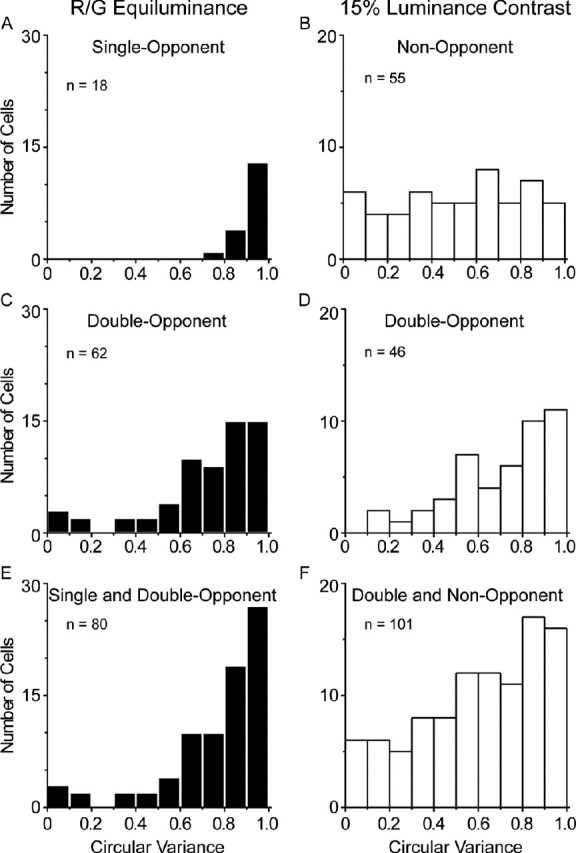
Population analysis of circular variance in single-opponent, double-opponent, and non-opponent populations. A, Single-opponent cells studied with equiluminant red–green (R/G) gratings. The average CV = 0.92 ± 0.01 (SE), because the single-opponent cells are so unselective for orientation. B, Non-opponent cells studied with luminance gratings (0.15 contrast). The average CV = 0.52 ± 0.04 (SE). C, Double-opponent cells studied with red–green equiluminant gratings. The average double-opponent CV for red–green equiluminance was 0.72 ± 0.03 (SE). D, Double-opponent cells studied with luminance gratings (0.15 contrast). The average double-opponent CV for luminance was 0.71 ± 0.03 (SE). E, Distribution of CV for the responses to red–green equiluminant stimuli, combining data from the single- and double-opponent populations. Mean CV = 0.76 ± 0.03 (SE). F, Distribution of CV for the responses to luminance (0.15 contrast) stimuli, combining data from the double- and non-opponent populations. Mean CV = 0.6 ± 0.03 (SE).

Discussion

Classes of chromatically opponent neurons and the double-opponent model

The orientation selectivity documented in this study, in addition to the bandpass spatial-frequency tuning for equiluminant chromatic gratings (Thorell et al., 1984; Johnson et al., 2001, 2004), adds considerable support to the spatial model of double-opponent neurons (Fig. 9A) we proposed previously (Shapley and Hawken, 2002; Johnson et al., 2004) [see also Solomon and Lennie (2007), their Box 4]. The two-dimensional spatial structure of the double-opponent model for simple cells is further supported by the direct measurements of the first-order chromatic kernels (Fig. 1A,B; supplemental Fig. 1A,B, available at www.jneurosci.org as supplemental material). Other models of double-opponent neurons with a circularly symmetric receptive field organization that is either single opponent with a non-opponent surround (Ts'o and Gilbert, 1988) [see also Solomon and Lennie (2007), their Box 4] or chromatically double opponent (Fig. 9B) (Billock, 1991; Conway and Livingstone, 2006) do not provide a satisfactory account of the double-opponent neurons we have described that are orientation and spatial-frequency selective with odd-symmetric receptive fields (Johnson et al., 2004). Receptive fields of neurons in the population of chromatically opponent neurons that are not orientation selective and respond best to low spatial-frequency color stimuli are well described by single-opponent models as shown in Figure 9C (Hubel and Wiesel, 1968; Lennie et al., 1990; Shapley and Hawken, 2002) [see Solomon and Lennie (2007), their Box 4].

Figure 9.

Models of double-opponent and single-opponent V1 neurons. A, Proposed sensitivity profile for an orientation-selective double-opponent simple cell. Here the spatial receptive field map is composed of subregions. Within each subregion, the L- and M-cones send signals that are opposite in sign, but are not precisely balanced in strength. Also, the spatial symmetry is no longer the same as for a center-surround neuron, but resembles the asymmetric or odd-symmetric spatial receptive fields of non-opponent cells. The diagram on the left illustrates the organization of the two-dimensional receptive field, and the right diagram shows the hypothetical spatial sensitivity profile. B, The classical model of a hypothetical double-opponent neuron that receives both excitation and inhibition from each cone input. Originally, it was thought these would be exactly balanced and arranged in a circular center-surround geometry as shown. C, Single-opponent red–green sensitive neurons receive inputs from L- and M-cones that are opposite in sign, but signals from each cone type are all the same sign. The diagram depicts the two-dimensional maps and spatial profiles for one type of single-opponent neuron (L+ center/M− surround “type 1” cell). Concentric, single-opponent models are adequate for parvocellular LGN neurons and many single-opponent V1 cells.

One of the critical components that distinguishes various proposals of double-opponent receptive field structure is the symmetry of the subunit structure (Shapley and Hawken, 2002; Solomon and Lennie, 2007). Analysis of a subset of the double-opponent simple cell receptive fields showed that many were odd-symmetric or asymmetric (Johnson et al., 2004), which is consistent with the predominance of asymmetric simple cell receptive fields mapped using achromatic stimuli in macaque V1 (Ringach, 2002). Girard and Morrone (1995) inferred from their results on human visual evoked potentials to gratings modulated in either luminance or red–green color that both color and luminance mechanisms have receptive fields that include asymmetric spatial substructure. It is also worth noting that Thorell et al. (1984) suggested a receptive field organization like the one in Figure 9A from their results on responses to flashed colored bars. Suppose that the cortex adopts the same design for non-opponent and chromatically opponent simple cell receptive fields; it would not be surprising that there is a close correspondence between the underlying receptive field structures of non-opponent and double-opponent neurons described in this study. It is important to note that there are differences in tuning between the double-opponent and non-opponent cortical receptive fields. In general, one feature of the non-opponent population is a lower average O/P ratio. We and our colleagues found that a non-orientation-selective, spatially low-pass, suppressive mechanism (called untuned suppression) plays an important role in establishing this facet of selectivity (Ringach et al., 2002, 2003; Xing et al., 2005). Perhaps untuned suppression is stronger in non-opponent than in double-opponent neurons.

Solomon and Lennie (2007) refer to the neurons with receptive fields we have called double-opponent cells as “weakly opponent.” However, we have presented evidence that double-opponent cells have a range of cone-opponent ratios and that there often are strongly opposing cone responses at the peak of double-opponent cells' spatial tuning curves (Johnson et al., 2004). The wide range of cone-opponent ratios in the double-opponent population will make different double-opponent cells selective for different colors. Such diversity in V1 color selectivities also has been observed by others (Lennie et al., 1990; Friedman et al., 2003) and is possibly a neural mechanism for the multiplicity of color-selective channels inferred from psychophysics (Webster and Mollon, 1994).

Function of single-opponent and double-opponent cells in color vision

There is an important role for edge-sensitive cells in color vision (Johnson et al., 2001; Friedman et al., 2003). Color induction, the complementary color appearance of a neutral gray area surrounded by a colored region, can be a strong effect (Gordon and Shapley, 2006). A striking demonstration of color induction is given in supplemental Figure 2 (available at www.jneurosci.org as supplemental material), an example of a color Chevreul illusion (cf. Ratliff, 1992). The edge-sensitive, double-opponent cells in V1 should support color induction. In addition to color induction, there are other perceptual phenomena that appear to require orientation-tuned color signals, for example, the perception of three-dimensional shape in orientation flow patterns (Zaidi and Li, 2006) and the perception of geometric illusions under chromatic equiluminant conditions (Wilson and Switkes, 2005; Hamburger et al., 2007). There are many other psychophysical and perceptual connections between color and form: spatially tuned masking with pure color patterns (Switkes et al., 1988; Losada and Mullen, 1994); orientation discrimination with pure color patterns (Webster et al., 1990; Beaudot and Mullen, 2005); tilt illusion with pure color patterns (Clifford et al., 2003); and color filling-in (Krauskopf, 1963).

Comparisons with previous work

Some early neurophysiological studies supported the concept of a spatially challenged color system. The older view was based in part on human psychophysics: the low-pass human color contrast sensitivity function (Mullen, 1985; De Valois and De Valois, 1988). Such psychophysical results were interpreted to mean that the neural tuning for color was likewise low-pass in spatial frequency. However, there is now a wealth of psychophysical evidence for orientation-sensitive, spatial-frequency-selective color-responsive cells (Switkes et al., 1988; Webster et al., 1990; Losada and Mullen, 1994; Clifford et al., 2003; Beaudot and Mullen, 2005). Recent human fMRI results on V1 cortex also have indicated the existence of orientation-tuned, color-responsive neurons in V1 (Engel, 2005; Sumner et al., 2008).

Hubel and Wiesel (1968) reported that many color-responsive neurons in macaque V1 lacked orientation specificity, although they did find some color-selective cells with orientation selectivity. Livingstone and Hubel (1987, 1988) suggested a link between color processing and the cytochrome oxidase (CO)-rich patches (blobs) and CO-poor interpatches (interblobs) in layer 2/3 of V1 (Wong-Riley, 1979; Livingstone and Hubel, 1984). Livingstone and Hubel (1984) proposed that the color-responsive cells in the blobs were double-opponent neurons with circular receptive fields that were not selective for stimulus orientation. Lennie et al. (1990) reported that some color-responsive V1 neurons showed evidence of spatial-frequency and orientation selectivity, but concluded that most V1 neurons preferred luminance modulation, and that V1 neurons that were most responsive to chromatic modulation had poor orientation selectivity and responded best to spatially uniform chromatic fields.

Another reading of cortical neurophysiology suggests that color information is not processed separately from spatial attributes in V1. Four previous studies suggested that color-responsive neurons can be orientation selective (Thorell et al., 1984; Leventhal et al., 1995; Yoshioka and Dow, 1996; Horwitz et al., 2007). Friedman et al. (2003) studied the responses to squares or bars of color of cells in V1 upper layers and V2 in the awake monkey. They found a substantial proportion (64%) of color-selective neurons in the upper layers of V1; most of these were most responsive to edges. They also found a smaller proportion of “color-surface-responsive cells,” cells that were not especially sensitive to edges. Their edge-responsive color cells were mostly orientation selective, whereas the surface-responding cells were not. Although more research is needed to establish the connection, it is a reasonable hypothesis that Friedman et al.'s (2003) edge-sensitive, color-selective cells were double-opponent cells, whereas their surface-responding cells were single-opponent neurons.

Conway and Livingstone (2006) reported approximately circularly symmetric double-opponent cells in macaque cortex. Their experiments involve mapping receptive fields by reverse correlation with cone-isolating stimuli, which were flashed, colored squares on a gray background. They selected neurons for study that responded well to the flashed, colored squares. It is possible that many, perhaps all, double-opponent cells that we studied do not respond to such stimuli. Most cells that Conway and Livingstone (2006) called double-opponent had very weak surround effects, and they stated that some of their double-opponent cells were “weakly orientation selective.” Therefore, it is possible that most of the cells they studied were what we would classify as single-opponent. Because of their weak surrounds, the double-opponent cells Conway and Livingstone describe would be inadequate to explain many of the color–form interactions we have discussed above.

Contrast invariance and orientation selectivity

Sclar and Freeman (1982) reported that orientation tuning was invariant with contrast, and since the studies of Ben-Yishai et al. (1995) and Troyer et al. (1998), there has been interest in the theoretical importance of this invariance [for example, Finn et al. (2007)]. Our results on orientation selectivity, color, and contrast reveal that contrast invariance is mostly a floor effect. Neurons of intermediate orientation selectivity become more selective at high contrast, as shown in Figure 7. Contrast noninvariance was observed both for non-opponent cells as well as for double-opponent cells. Our findings replicate in monkey V1 the findings of Alitto and Usrey (2004) in ferret V1. We do not know the mechanism for the sharpening of orientation selectivity at higher contrast, but we suspect it is related to the contrast dependence of corticocortical interactions. Whatever the mechanism, the greater orientation selectivity at higher contrast had important consequences in our experiments. The implication of contrast noninvariance is that it is necessary to compare orientation selectivities of V1 neurons to patterns of comparable cone contrast to assess the relative efficacy of colored and achromatic stimuli for conveying orientation-dependent signals. When we did the matched comparison, we found that the orientation selectivity of the double-opponent population was approximately the same for color and luminance.

References

- Alitto HJ, Usrey WM. Influence of contrast on orientation and temporal frequency tuning in ferret primary visual cortex. J Neurophysiol. 2004;91:2797–2808. doi: 10.1152/jn.00943.2003. [DOI] [PubMed] [Google Scholar]
- Beaudot WH, Mullen KT. Orientation selectivity in luminance and color vision assessed using 2-d band-pass filtered spatial noise. Vision Res. 2005;45:687–696. doi: 10.1016/j.visres.2004.09.023. [DOI] [PubMed] [Google Scholar]
- Ben-Yishai R, Bar-Or RL, Sompolinsky H. Theory of orientation tuning in visual cortex. Proc Natl Acad Sci U S A. 1995;92:3844–3848. doi: 10.1073/pnas.92.9.3844. [DOI] [PMC free article] [PubMed] [Google Scholar]
- Billock VA. The relationship between simple and double-opponent cells. Vision Res. 1991;31:33–42. doi: 10.1016/0042-6989(91)90070-l. [DOI] [PubMed] [Google Scholar]
- Brainard D. Color constancy. In: Chalupa L, Werner J, editors. Visual neuroscience. Cambridge, MA: MIT; 2002. pp. 948–961. [Google Scholar]
- Clifford CW, Spehar B, Solomon SG, Martin PR, Zaidi Q. Interactions between color and luminance in the perception of orientation. J Vis. 2003;3:106–115. doi: 10.1167/3.2.1. [DOI] [PubMed] [Google Scholar]
- Conway BR, Livingstone MS. Spatial and temporal properties of cone signals in alert macaque primary visual cortex. J Neurosci. 2006;26:10826–10846. doi: 10.1523/JNEUROSCI.2091-06.2006. [DOI] [PMC free article] [PubMed] [Google Scholar]
- Daw NW. Visual response to gradients of varying colour and equal luminance. Nature. 1964;203:215–216. doi: 10.1038/203215a0. [DOI] [PubMed] [Google Scholar]
- Daw NW. Goldfish retina: organization for simultaneous color contrast. Science. 1967;158:942–944. doi: 10.1126/science.158.3803.942. [DOI] [PubMed] [Google Scholar]
- De Valois RL. Analysis and coding of color vision in the primate visual system. Cold Spring Harb Symp Quant Biol. 1965;30:567–579. doi: 10.1101/sqb.1965.030.01.055. [DOI] [PubMed] [Google Scholar]
- De Valois RL, De Valois KK. In: Spatial vision. Broadbent DE, Mackintosh NJ, Posner MI, Tulving E, Weiskrantz K, editors. Vol 14. New York: Oxford UP; 1988. Oxford Psychology Series. [Google Scholar]
- Engel SA. Adaptation of oriented and unoriented color-selective neurons in human visual areas. Neuron. 2005;45:613–623. doi: 10.1016/j.neuron.2005.01.014. [DOI] [PubMed] [Google Scholar]
- Estévez O, Spekreijse H. The “silent substitution” method in visual research. Vision Res. 1982;22:681–691. doi: 10.1016/0042-6989(82)90104-3. [DOI] [PubMed] [Google Scholar]
- Finn IM, Priebe NJ, Ferster D. The emergence of contrast-invariant orientation tuning in simple cells of cat visual cortex. Neuron. 2007;54:137–152. doi: 10.1016/j.neuron.2007.02.029. [DOI] [PMC free article] [PubMed] [Google Scholar]
- Forbes A, Burleigh S, Neyland M. Electric responses to color shift in frog and turtle retina. J Neurophysiol. 1955;18:517–535. doi: 10.1152/jn.1955.18.6.517. [DOI] [PubMed] [Google Scholar]
- Friedman HS, Zhou H, von der Heydt R. The coding of uniform colour figures in monkey visual cortex. J Physiol. 2003;548:593–613. doi: 10.1113/jphysiol.2002.033555. [DOI] [PMC free article] [PubMed] [Google Scholar]
- Gegenfurtner KR, Kiper DC. Color vision. Annu Rev Neurosci. 2003;26:181–206. doi: 10.1146/annurev.neuro.26.041002.131116. [DOI] [PubMed] [Google Scholar]
- Gegenfurtner KR, Kiper DC, Fenstemaker SB. Processing of color, form and motion in macaque V2. Vis Neurosci. 1996;13:161–172. doi: 10.1017/s0952523800007203. [DOI] [PubMed] [Google Scholar]
- Girard P, Morrone MC. Spatial structure of chromatically opponent receptive fields in the human visual system. Vis Neurosci. 1995;12:103–116. doi: 10.1017/s0952523800007355. [DOI] [PubMed] [Google Scholar]
- Gordon J, Shapley R. Brightness contrast inhibits color induction: evidence for a new kind of color theory. Spat Vis. 2006;19:133–146. doi: 10.1163/156856806776923498. [DOI] [PubMed] [Google Scholar]
- Hamburger K, Hansen T, Gegenfurtner KR. Geometric-optical illusions at isoluminance. Vision Res. 2007;47:3276–3285. doi: 10.1016/j.visres.2007.09.004. [DOI] [PubMed] [Google Scholar]
- Hawken MJ, Parker AJ, Lund JS. Laminar organization and contrast sensitivity of direction-selective cells in the striate cortex of the Old World monkey. J Neurosci. 1988;8:3541–3548. doi: 10.1523/JNEUROSCI.08-10-03541.1988. [DOI] [PMC free article] [PubMed] [Google Scholar]
- Horwitz GD, Chichilnisky EJ, Albright TD. Cone inputs to simple and complex cells in V1 of awake macaque. J Neurophysiol. 2007;97:3070–3081. doi: 10.1152/jn.00965.2006. [DOI] [PubMed] [Google Scholar]
- Hubel DH, Wiesel TN. Receptive fields, binocular interaction and functional architecture in the cat's visual cortex. J Physiol. 1962;160:106–154. doi: 10.1113/jphysiol.1962.sp006837. [DOI] [PMC free article] [PubMed] [Google Scholar]
- Hubel DH, Wiesel TN. Receptive fields and functional architecture of monkey striate cortex. J Physiol. 1968;195:215–243. doi: 10.1113/jphysiol.1968.sp008455. [DOI] [PMC free article] [PubMed] [Google Scholar]
- Hurlbert A, Wolf K. Color contrast: a contributory mechanism to color constancy. Prog Brain Res. 2004;144:147–160. doi: 10.1016/s0079-6123(03)14410-x. [DOI] [PubMed] [Google Scholar]
- Hyman J. The objective eye. Chicago: University of Chicago; 2006. [Google Scholar]
- Johnson EN, Hawken MJ, Shapley R. The spatial transformation of color in the primary visual cortex of the macaque monkey. Nat Neurosci. 2001;4:409–416. doi: 10.1038/86061. [DOI] [PubMed] [Google Scholar]
- Johnson EN, Hawken MJ, Shapley R. Cone inputs in macaque primary visual cortex. J Neurophysiol. 2004;91:2501–2514. doi: 10.1152/jn.01043.2003. [DOI] [PubMed] [Google Scholar]
- Katz D. In: The world of colour. MacLeod RB, Fox CW, translators. London: Kegan, Paul, Trench, Truebner; 1935. [Google Scholar]
- Krauskopf J. Effect of retinal image stabilization on the appearance of heterochromatic targets. J Opt Soc Am. 1963;53:741–744. doi: 10.1364/josa.53.000741. [DOI] [PubMed] [Google Scholar]
- Lennie P, Krauskopf J, Sclar G. Chromatic mechanisms in striate cortex of macaque. J Neurosci. 1990;10:649–669. doi: 10.1523/JNEUROSCI.10-02-00649.1990. [DOI] [PMC free article] [PubMed] [Google Scholar]
- Leventhal AG, Thompson KG, Liu D, Zhou Y, Ault SJ. Concomitant sensitivity to orientation, direction, and color of cells in layers 2, 3, and 4 of monkey striate cortex. J Neurosci. 1995;15:1808–1818. doi: 10.1523/JNEUROSCI.15-03-01808.1995. [DOI] [PMC free article] [PubMed] [Google Scholar]
- Livingstone MS, Hubel DH. Anatomy and physiology of a color system in the primate visual cortex. J Neurosci. 1984;4:309–356. doi: 10.1523/JNEUROSCI.04-01-00309.1984. [DOI] [PMC free article] [PubMed] [Google Scholar]
- Livingstone MS, Hubel DH. Psychophysical evidence for separate channels for the perception of form, color, movement, and depth. J Neurosci. 1987;7:3416–3468. doi: 10.1523/JNEUROSCI.07-11-03416.1987. [DOI] [PMC free article] [PubMed] [Google Scholar]
- Livingstone M, Hubel D. Segregation of form, color, movement, and depth: anatomy, physiology, and perception. Science. 1988;240:740–749. doi: 10.1126/science.3283936. [DOI] [PubMed] [Google Scholar]
- Losada MA, Mullen KT. The spatial tuning of chromatic mechanisms identified by simultaneous masking. Vision Res. 1994;34:331–341. doi: 10.1016/0042-6989(94)90091-4. [DOI] [PubMed] [Google Scholar]
- Mardia KV. Statistics of directional data. London: Academic; 1972. [Google Scholar]
- Michael CR. Laminar segregation of color cells in the monkey's striate cortex. Vision Res. 1985;25:415–423. doi: 10.1016/0042-6989(85)90067-7. [DOI] [PubMed] [Google Scholar]
- Mullen KT. The contrast sensitivity of human colour vision to red-green and blue-yellow chromatic gratings. J Physiol. 1985;359:381–400. doi: 10.1113/jphysiol.1985.sp015591. [DOI] [PMC free article] [PubMed] [Google Scholar]
- Ratliff F. Paul Signac and color in neo-impressionism. New York: Rockefeller UP; 1992. p. 62. [Google Scholar]
- Reid RC, Shapley RM. Spatial structure of cone inputs to receptive fields in primate lateral geniculate nucleus. Nature. 1992;356:716–718. doi: 10.1038/356716a0. [DOI] [PubMed] [Google Scholar]
- Reid RC, Shapley RM. Space and time maps of cone photoreceptor signals in macaque lateral geniculate nucleus. J Neurosci. 2002;22:6158–6175. doi: 10.1523/JNEUROSCI.22-14-06158.2002. [DOI] [PMC free article] [PubMed] [Google Scholar]
- Ringach DL. Spatial structure and symmetry of simple-cell receptive fields in macaque primary visual cortex. J Neurophysiol. 2002;88:455–463. doi: 10.1152/jn.2002.88.1.455. [DOI] [PubMed] [Google Scholar]
- Ringach DL, Sapiro G, Shapley R. A subspace reverse-correlation technique for the study of visual neurons. Vision Res. 1997;37:2455–2464. doi: 10.1016/s0042-6989(96)00247-7. [DOI] [PubMed] [Google Scholar]
- Ringach DL, Shapley RM, Hawken MJ. Orientation selectivity in macaque V1: diversity and laminar dependence. J Neurosci. 2002;22:5639–5651. doi: 10.1523/JNEUROSCI.22-13-05639.2002. [DOI] [PMC free article] [PubMed] [Google Scholar]
- Ringach DL, Hawken MJ, Shapley R. Dynamics of orientation tuning in macaque V1: the role of global and tuned suppression. J Neurophysiol. 2003;90:342–352. doi: 10.1152/jn.01018.2002. [DOI] [PubMed] [Google Scholar]
- Schluppeck D, Engel SA. Color opponent neurons in V1: a review and model reconciling results from imaging and single-unit recording. J Vis. 2002;2:480–492. doi: 10.1167/2.6.5. [DOI] [PubMed] [Google Scholar]
- Sclar G, Freeman RD. Orientation selectivity in the cat's striate cortex is invariant with stimulus contrast. Exp Brain Res. 1982;46:457–461. doi: 10.1007/BF00238641. [DOI] [PubMed] [Google Scholar]
- Shapley R, Hawken M. Parallel retinocortical channels and luminance. In: Gegenfurtner K, Sharpe L, editors. Color: from genes to perception. Cambridge, UK: Cambridge UP; 1999. pp. 221–234. [Google Scholar]
- Shapley R, Hawken M. Neural mechanisms for color perception in the primary visual cortex. Curr Opin Neurobiol. 2002;12:426–432. doi: 10.1016/s0959-4388(02)00349-5. [DOI] [PubMed] [Google Scholar]
- Skottun BC, De Valois RL, Grosof DH, Movshon JA, Albrecht DG, Bonds AB. Classifying simple and complex cells on the basis of response modulation. Vision Res. 1991;31:1079–1086. doi: 10.1016/0042-6989(91)90033-2. [DOI] [PubMed] [Google Scholar]
- Solomon SG, Lennie P. The machinery of colour vision. Nat Rev Neurosci. 2007;8:276–286. doi: 10.1038/nrn2094. [DOI] [PubMed] [Google Scholar]
- Sumner P, Anderson EJ, Sylvester R, Haynes JD, Rees G. Combined orientation and colour information in human V1 for both L-M and S-cone chromatic axes. Neuroimage. 2008;39:814–824. doi: 10.1016/j.neuroimage.2007.09.013. [DOI] [PubMed] [Google Scholar]
- Switkes E, Bradley A, De Valois KK. Contrast dependence and mechanisms of masking interactions among chromatic and luminance gratings. J Opt Soc Am A. 1988;5:1149–1162. doi: 10.1364/josaa.5.001149. [DOI] [PubMed] [Google Scholar]
- Thorell LG, De Valois RL, Albrecht DG. Spatial mapping of monkey V1 cells with pure color and luminance stimuli. Vision Res. 1984;24:751–769. doi: 10.1016/0042-6989(84)90216-5. [DOI] [PubMed] [Google Scholar]
- Troyer TW, Krukowski AE, Priebe NJ, Miller KD. Contrast-invariant orientation tuning in cat visual cortex: thalamocortical input tuning and correlation-based intracortical connectivity. J Neurosci. 1998;18:5908–5927. doi: 10.1523/JNEUROSCI.18-15-05908.1998. [DOI] [PMC free article] [PubMed] [Google Scholar]
- Ts'o DY, Gilbert CD. The organization of chromatic and spatial interactions in the primate striate cortex. J Neurosci. 1988;8:1712–1727. doi: 10.1523/JNEUROSCI.08-05-01712.1988. [DOI] [PMC free article] [PubMed] [Google Scholar]
- Wachtler T, Sejnowski TJ, Albright TD. Representation of color stimuli in awake macaque primary visual cortex. Neuron. 2003;37:681–691. doi: 10.1016/s0896-6273(03)00035-7. [DOI] [PMC free article] [PubMed] [Google Scholar]
- Webster MA, De Valois KK, Switkes E. Orientation and spatial-frequency discrimination for luminance and chromatic gratings. J Opt Soc Am A. 1990;7:1034–1049. doi: 10.1364/josaa.7.001034. [DOI] [PubMed] [Google Scholar]
- Webster MA, Mollon JD. The influence of contrast adaptation on color appearance. Vision Res. 1994;34:1993–2020. doi: 10.1016/0042-6989(94)90028-0. [DOI] [PubMed] [Google Scholar]
- Wilson JA, Switkes E. Integration of differing chromaticities in early and midlevel spatial vision. J Opt Soc Am A. 2005;22:2169–2181. doi: 10.1364/josaa.22.002169. [DOI] [PubMed] [Google Scholar]
- Wong-Riley M. Changes in the visual system of monocularly sutured or enucleated cats demonstrated with cytochrome oxidase histochemistry. Brain Res. 1979;171:11–28. doi: 10.1016/0006-8993(79)90728-5. [DOI] [PubMed] [Google Scholar]
- Xing D, Ringach DL, Shapley R, Hawken MJ. Correlation of local and global orientation and spatial frequency tuning in macaque V1. J Physiol. 2004;557:923–933. doi: 10.1113/jphysiol.2004.062026. [DOI] [PMC free article] [PubMed] [Google Scholar]
- Xing D, Shapley RM, Hawken MJ, Ringach DL. The effect of stimulus size on the dynamics of orientation selectivity in macaque V1. J Neurophysiol. 2005;94:799–812. doi: 10.1152/jn.01139.2004. [DOI] [PubMed] [Google Scholar]
- Yoshioka T, Dow BM. Color, orientation and cytochrome oxidase reactivity in areas V1, V2 and V4 of macaque monkey visual cortex. Behav Brain Res. 1996;76:71–88. doi: 10.1016/0166-4328(95)00184-0. [DOI] [PubMed] [Google Scholar]
- Zaidi Q, Li A. Three-dimensional shape perception from chromatic orientation flows. Vis Neurosci. 2006;23:323–330. doi: 10.1017/S0952523806233170. [DOI] [PMC free article] [PubMed] [Google Scholar]