Generalized Replica Exchange Method

Abstract

We present a powerful replica exchange method, particularly suited to first-order phase transitions associated with the backbending in the statistical temperature, by merging an optimally designed generalized ensemble sampling with replica exchanges. The key ingredients of our method are parametrized effective sampling weights, smoothly joining ordered and disordered phases with a succession of unimodal energy distributions by transforming unstable or metastable energy states of canonical ensembles into stable ones. The inverse mapping between the sampling weight and the effective temperature provides a systematic way to design the effective sampling weights and determine a dynamic range of relevant parameters. Illustrative simulations on Potts spins with varying system size and simulation conditions demonstrate a comprehensive sampling for phase-coexistent states with a dramatic acceleration of tunneling transitions. A significant improvement over the power-law slowing down of mean tunneling times with increasing system size is obtained, and the underlying mechanism for accelerated tunneling is discussed.

INTRODUCTION

Recently, the temperature replica exchange method^{1, 2} (tREM) [also called parallel tempering³ (PT)] has become a key workhorse for equilibrium sampling of a variety of complex systems across multidisciplinary fields.^{4, 5, 6, 7, 8} Simulating a set of replicas of the same system at a distribution of temperatures and swapping configurations among replicas offers an effective means of avoiding trapping in local minima and mitigating broken ergodicity at low temperatures.⁹

A great deal of effort^{10, 11, 12, 13, 14, 15, 16, 17, 18, 19, 20, 21, 22, 23, 24, 25, 26, 27} has been devoted to improving the efficiency of the standard tREM. One of the debated issues is its applicability to systems displaying strong phase transitions, around which metastable or unstable energy states intervene between two macroscopic phases.²⁸ The standard tREM struggles to attain its maximum power in the vicinity of a first-order phase transition, in which canonical energy distributions are effectively disjointed by an energy gap corresponding to a latent heat. Since the acceptance probability of replica exchanges is determined by the energy overlap of neighboring replicas an energy gap between P_T<Tc(E) and P_T>Tc(E) around the critical temperature T_c, P_T(E) being the canonical probability density function (PDF) at the temperature T, significantly impairs replica exchanges.

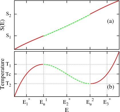
More fundamentally, the failure of the tREM in first-order phase transitions is intimately connected to an anomalous behavior of the microcanonical entropy, S(E), across the transition region. In many finite size systems, such as spins,²⁹ nuclei fragmentations,^{30, 31} model proteins,^{32, 33, 34} and atomic clusters,^{8, 35, 36}S(E) shows a convex dip, i.e., ∂²S∕∂E²>0,³⁰ across the transition region, as sketched in Fig. 1a. Stemming from this convex “intruder” in S(E), the statistical temperature or microcanonical temperature,

$$T_S\left(E\right)={\left(\partial S∕\partial E\right)}^{-1},$$ (1)

exhibits a negative slope region in Fig. 1b, the so called backbending or S-loop.^{32, 33, 35, 36} The existence of the backbending has been verified in recent experiments on nuclear fragmentation³⁷ and cluster melting,³⁸ and its physical origin has been attributed to avoiding a “static” phase coexistence due to the free energy cost forming interfaces.

Figure 1.

A schematic representation of (a) the convex dip i.e., ∂²S∕∂E²>0 in S(E) and (b) the backbending in T_S(E). Intermediate energy states between $E_u^1$ and $E_u^2$ are unstable in the canonical ensemble and become inaccessible as the system size increases.

The backbending in T_S(E) manifests a bimodal structure in P_T(E)∝e^−βF(E,T), F(E,T)=E−TS(E) being the Helmhotz free energy density and β=[k_BT]⁻¹ (k_B=1).³⁹ With the stationary points, $E_i^{*}$, of F(E,T) determined by an extremum condition, $T_S\left(E_i^{*}\right)=T$, with $E_1^{*}<E_2^{*}<E_3^{*}$ for T₂<T<T₁,^{30, 34}P_T(E) becomes double peaked at $E_1^{*}$ and $E_3^{*}$ with a minimum at $E_2^{*}$. The stability condition, $\beta {\mathcal{F}}^{″}\left(E\right)={\beta }^2{T}_S^{\prime }\left(E\right)$, the prime being a differentiation with respect to E, reveals that the intermediate energy states between $E_u^1$ and $E_u^2$ in Fig. 1b corresponding to the backbending region in T_S(E) are intrinsically unstable for the canonical ensemble.

For a small system size, L, the canonical ensemble can sample both free energy minima, at $E_1^{*}$ and $E_3^{*}$, across the free energy barrier at $E_2^{*}$. However, as L increases, the backbending energy region becomes inaccessible due to a high free energy barrier, implying that tunneling transitions between the two macroscopic phases become unlikely, and P_T(E) becomes localized around $E_1^{*}$ or $E_3^{*}$, depending on whether T<T_c or not. Accordingly, the acceptance of replica exchanges for a pair of inverse temperatures, β and β^′, close to β_c=1∕T_c, becomes exponentially suppressed as

$$A\left(\beta E;{\beta }^{\prime }{E}^{\prime }\right)=\text{min}\left[1,e^{\Delta \beta \left(E^{\prime }-E\right)}\right]\approx e^{-\left|\Delta \beta \Delta E^{*}\right|},$$ (2)

where Δβ=β^′−β and $\Delta E^{*}=E_3^{*}-E_1^{*}$. Notice that ΔE=E^′−E≈ΔE^* for β>β_c>β^′ and ΔE≈−ΔE^* for β<β_c<β^′ since P_T(E) is centered at $E_1^{*}$ for β>β_c and $E_3^{*}$ for β<β_c. We conclude that the instability of the canonical ensemble to the negative slope region in T_S(E) is the main cause of the poor acceptance of replica exchanges in the standard tREM, with increasing system size.

An obvious way to restore the full power of replica exchanges is to utilize a noncanonical ensemble, avoiding the instability to the negative slope region in T_S(E), and allowing a unimodal energy distribution. The Gaussian ensemble approach⁴⁰ and its parallel version⁴¹ accomplish this goal by multiplying the Boltzmann factor by a Gaussian in energy.

In this paper, we propose a general framework to systematically build up optimized noncanonical ensembles, transforming unstable or metastable energy states of canonical ensembles into stable states in the presence of the backbending in T_S(E). Exploiting the one-to-one correspondence between the sampling weight and the effective temperatures,^{42, 43, 44, 45, 46} we develop an inverse mapping strategy, which determines a set of optimal generalized ensemble weights from the parametrized effective temperatures tailored to naturally bridge between ordered and disordered phases via a succession of unimodal energy distributions.

Simulations on Potts spins with varying system size, L, demonstrate that optimally designed generalized ensembles combined with replica exchanges (gREM) yield a dramatic acceleration of tunneling transitions and enable a comprehensive sampling of the phase transition region. A detailed mechanism for an order of magnitude acceleration in tunneling is discussed, with a quantitative performance comparison to the Wang–Landau (WL) method. Finite size scaling analysis reveals that the mean tunneling time, τ_E, can be as favorable as ∝L^2d characteristic of a perfect random walk in flat histogram methods.^{47, 48, 49}

The paper is organized as follows: In Sec. 2, the theory of the gREM is presented, with detailed simulation protocols. In Sec. 3, the performance of the gREM is examined and quantitatively compared to that of WL sampling,⁴⁸ for Potts spin systems under various simulation conditions. Conclusions and a brief summary are presented in Sec. 4.

GENERALIZED REPLICA EXCHANGE METHOD

Inverse mapping strategy

The key idea of the gREM is to construct a set of generalized ensemble weights, W_α(E,λ_α) (α=1,2,…,M), which, as the parameter λ_α varies, successively access the unstable energy region between $E_u^1$ and $E_u^2$ in Fig. 1b. Here α and M are the replica index and the number of replicas, respectively. An important relation in the design of optimal weights is the inverse mapping between the W_α and the effective temperature

$$T_{\alpha }\left(E;{\lambda }_{\alpha }\right)={\left[\partial w_{\alpha }∕\partial E\right]}^{-1},$$ (3)

w_α=−ln W_α being the generalized effective potential. Notice that the definition of the effective temperature in Eq. 3 is analogous to that of the statistical temperature in Eq. 1. Based on the one-to-one correspondence in Eq. 3, the effective temperature completely determines the sampling weight up to a constant through the inverse mapping,

$$w_{\alpha }\left(E;{\lambda }_{\alpha }\right)={\int }^{E}1∕T_{\alpha }\left(z;{\lambda }_{\alpha }\right)dz.$$ (4)

A necessary and sufficient condition on T_α(E;λ_α), such that unstable or metastable energy states of the canonical ensemble between $E_u^1$ and $E_u^2$ are transformed into stable ones with a unimodal PDF, is derived by identifying an extremum, $E_{\alpha }^{*}$, of a generalized free energy density, βF_α(E)=w_α(E)−S(E),

$$T_{\alpha }\left(E_{\alpha }^{*};{\xi }_{\alpha }\right)=T_S\left(E_{\alpha }^{*}\right)=T_{\alpha }^{*},$$ (5)

and a stability condition

$$\beta {\mathcal{F}}_{\alpha }^{″}\left(E_{\alpha }^{*}\right)=\left({\gamma }_S-{\gamma }_{\alpha }\right)∕T_{\alpha }^{*2},$$ (6)

where ${\gamma }_S=T_S^{\prime }\left(E_{\alpha }^{*}\right)$ and ${\gamma }_{\alpha }=T_{\alpha }^{\prime }\left(E_{\alpha }^{*}\right)$, and the prime denotes differentiation with respect to E. The primary finding in both Eqs. 5, 6 is that the stationary points of F_α(E), $E_{\alpha }^{*}$, are determined as the crossing points between T_α(E;λ_α) and T_S(E) in two-dimensional (E,T) space, and the parameter γ_α modulates the stability of $E_{\alpha }^{*}$ via ${\gamma }_{\alpha }=T_{\alpha }^{\prime }\left(E_{\alpha }^{*};{\lambda }_{\alpha }\right)$. Based on Eqs. 5, 6 we find that a unimodal distribution in the generalized PDF (GPDF), i.e., P_α(E)=e^−βF_α, can arise from forming the unique crossing point, $E_{\alpha }^{*}$, between T_S(E) and T_α(E;λ_α), subject to ${\gamma }_{\alpha }\left(E_{\alpha }^{*}\right)<{\gamma }_S\left(E_{\alpha }^{*}\right)$.

More quantitatively, expanding the GPDF up to second order yields

$$P_{\alpha }\left(E;{\lambda }_{\alpha }\right)\approx \text{exp}\left\{-{\left(E-E_{\alpha }^{*}\right)}^2∕2{\sigma }_{\gamma }\right\},$$ (7)

${\sigma }_{\gamma }=T_{\alpha }^{*2}∕\left({\gamma }_S-{\gamma }_{\alpha }\right)$, illuminating that the “stable” in Fig. 2, with γ_α<γ_S, generates a Gaussian PDF centered at $E_{\alpha }^{*}$ with the positive σ_γ even for a negative γ_S. As γ_α further decreases to −∞, the Gaussian in Eq. 7 approaches $\delta \left(E-E_{\alpha }^{*}\right)$ corresponding to the microcanonical ensemble case. On the other hand, P_α(E) becomes locally flat around $E_{\alpha }^{*}$, with γ_α=γ_S (“marginal” in Fig. 2). The crossing point, $E_{\alpha }^{*}$, becomes unstable for γ_α>γ_S as in the canonical ensemble.

Figure 2.

Statistical temperature T_S(E) and effective temperatures $T_{\alpha }\left(E\right)=T_c+{\gamma }_{\alpha }\left(E-E_2^{*}\right)$ with varying γ₀, ${\gamma }_0=T_{\alpha }^{\prime }\left(E_2^{*}\right)$. Unstable energy states around $E_2^{*}$ in the canonical ensemble (γ₀=0) become stable in the generalized ensemble of Eq. 10 with ${\gamma }_0<{\gamma }_S^{\text{min}}=T_S^{\prime }\left(E_2^{*}\right)$. Marginal corresponds to ${\gamma }_0={\gamma }_S^{\text{min}}$.

Linear effective temperature: Tsallis weight

The simplest parametrization scheme for forming stable crossing points between T_α(E;λ_α) and T_S(E) is to align linear effective temperatures in parallel with the constant slope, λ₀ [see Fig. 3a], as

$$T_{\alpha }\left(E;{\lambda }_{\alpha }\right)={\lambda }_{\alpha }+{\gamma }_0\left(E-E_0\right),$$ (8)

the control parameter λ_α being the T-intercept at an arbitrarily chosen E₀. To form the unique stable crossing point $E_{\alpha }^{*}$ in each replica, γ₀ must be less than the minimum slope ${\gamma }_S^{\text{min}}$, ${\gamma }_S^{\text{min}}=\text{min}\left\{T_S^{\prime }\left(E\right)\right\}$ being the minimum slope of T_S(E) for the sampled energy region. Since T_S(E) is monotonically increasing except for the transition region, in most cases a proper γ₀ is easily guessed from the approximate T_S(E) by connecting a few points of $\left[\tilde{U}\left(T\right),T\right]$, $\tilde{U}\left(T\right)$ being an average energy of a short canonical run at T. For example, γ₀ can be simply chosen as ${\gamma }_L=\left(T_M-T_1\right)∕\left({\tilde{U}}_1-{\tilde{U}}_M\right)$, T₁ and T_M being the lowest and highest temperature, and ${\tilde{U}}_{\alpha }=\tilde{U}\left(T_{\alpha }\right)$.

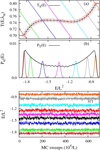
Figure 3.

(a) Most probable energy set $\left[E_{\alpha }^{*},T_{\alpha }^{*}\right]$ (squares) determined by the gREM₃ for 10⁷ MCS and T_S(E) (solid line) determined by the STMC simulation and effective temperatures T_α(E;λ_α), (b) resulting GPDFs P_α(E) and P_T(E) (solid line) for Potts spins with L=64, and (c) energy trajectories sampled by Eq. 10. In both (a) and (b), α=1, 5, 10, 15, 20, 25, and 30 from left to right. α=1, 5, 10, 13, 15, 17, 20, 25, and 30 from down to up in (c).

Once γ₀ is fixed the dynamic range of λ_α is determined to cover the interesting temperature range between T₁ and T_M as λ₁=T₁ and ${\lambda }_M=T_M-{\lambda }_0\left({\tilde{U}}_M-{\tilde{U}}_1\right)$, with $E_0={\tilde{U}}_1$. The first and Mth effective temperatures are chosen to cross $\left[{\tilde{U}}_1,T_1\right]$ and $\left[{\tilde{U}}_M,T_M\right]$, respectively. Then, the intermediate values of λ_α (1<α<M) are determined by equally dividing the parameter space as

$${\lambda }_{\alpha }={\lambda }_1+\left(\alpha -1\right)\Delta \lambda$$ (9)

and Δλ=(λ_M−λ₁)∕(M−1).

Interestingly, the linear effective temperature of Eq. 8 produces a generic form of the Tsallis weight^{50, 51, 52}

$$W_{\alpha }\left(E;{\lambda }_{\alpha }\right)\sim {\left[{\lambda }_{\alpha }+{\gamma }_0\left(E-E_0\right)\right]}^{-1∕{\gamma }_0}.$$ (10)

Identifying γ₀ and λ_α by (q−1) and ${\beta }_{\alpha }^{-1}$, respectively, q being the nonextensivity parameter, recovers the original form of the Tsallis weight proposed in nonextensive statistical mechanics.⁵⁰ Thus the gREM with the linear effective temperature of Eq. 8 is basically equivalent to the Tsallis-weight based REM, previously presented in the form of the generalized PT,¹⁴q-REM,¹⁵ and Tsallis-REM.⁵³

However, it should be noted that the parametrized Tsallis weights in the gREM are targeted to transform unstable and metastable energy states of the canonical ensemble into stable ones, resulting in much narrower energy distributions than the canonical PDFs. On the other hand, other variants^{14, 15, 53, 54} of the Tsallis-weight based REM are mainly focused on producing more delocalized energy distributions to increase an acceptance of replica exchanges. This is why the gREM utilizes λ_α as a control parameter rather than q in the conventional implementation.

Another advantage of the gREM is that the inverse mapping enables a systematic selection of relevant parameters, which is particularly beneficial for the negative slope region of T_S(E). The dynamic range of λ_α lies between λ₁ and λ_M determined by two short canonical runs at T₁ and T_M, respectively. The inverse mapping is a general framework for the combination of any generalized ensemble sampling with replica exchanges. Depending on the profile of T_S(E), characteristic of the phase transition, different types of effective temperatures can be designed to produce optimal weights. In the limit, γ₀→0, the gREM recovers the tREM running on temperatures λ_α, denoting W_α(E;λ_α)∼e^{−(E−E₀)∕λ_α}.

Simulation protocols of the gREM

Detailed simulation protocols of the gREM are outlined as follows.

• (i)Perform short canonical runs at several temperatures between T₁ and T_M to determine the data set, $\left[{\tilde{U}}_{\alpha },T_{\alpha }\right]$. Select a proper γ₀ to be less than ${\gamma }_S^{\text{min}}$ and determine λ_α by employing Eq. 9 between λ₁=T₁ and ${\lambda }_M=T_M-{\gamma }_0\left({\tilde{U}}_M-{\tilde{U}}_1\right)$, with $E_0={\tilde{U}}_1$.
• (ii)
  Run the gREM simulation in each replica by making trial moves in configuration space with the acceptance,

  $$A_{\text{intra}}\left(\mathbf{x}\to {\mathbf{x}}^{\prime }\right)=\text{min}\left[1,e^{w_{\alpha }\left(E\right)-w_{\alpha }\left(E^{\prime }\right)}\right].$$ (11)

  Every fixed time step, attempt a replica exchange between neighboring replicas with the acceptance

  $$A_{\text{inter}}\left(\alpha ;\mathbf{x}{\mathbf{x}}^{\prime }\right)=\text{min}\left[1,\text{exp}\left({\Delta }_{\alpha }\right)\right],$$ (12)

  $${\Delta }_{\alpha }=w_{\alpha +1}\left(E^{\prime }\right)-w_{\alpha +1}\left(E\right)+w_{\alpha }\left(E\right)-w_{\alpha }\left(E^{\prime }\right).$$
• (iii)Once a sufficiently long production run has been performed, calculate the entropy estimate $\tilde{S}\left(E\right)$ by joining multiple generalized ensemble runs via the weighted histogram analysis method (WHAM).⁵⁵

NUMERICAL SIMULATIONS AND RESULTS

To illustrate how effectively the gREM works around a typical first-order transition, we have chosen eight-state Potts spins as a benchmark, with the energy E=−∑_⟨ij⟩δ(S_i,S_j),⁵⁶ in which the sum runs over the nearest-neighbor spins on an L×L square lattice and Kronecker δ takes the value one if S_i=S_j and zero otherwise. Here S_i=1,2,…, Q=8 are spin variables.

Characteristic features of the gREM

To determine the dynamic range of λ_α and the optimal value of γ₀ we first performed short canonical Monte Carlo (MC) simulations for 2×10⁴ MC sweeps (MCSs) at T₁=0.7 and T_M=0.8, which determine ${\tilde{U}}_1=-7507.8$ and${\tilde{U}}_M=-3438.7$. Here one MCS means L² MC trial moves of all spins. Based on ${\gamma }_L=\left(T_M-T_1\right)∕\left({\tilde{U}}_1-{\tilde{U}}_M\right)\approx -2.5\times {10}^{-5}$ we performed various gREM simulations with varying γ₀ for L=64, as summarized in Table 1. Replica exchanges were attempted every L MC moves and the ground state was used as the initial configuration in all replicas.

Table 1.

Simulation parameters and mean tunneling times τ_E for the gREM and the WL simulations for Potts spins with L=64. t_S represents a total simulation time in the gREM and a time spent for refining $\tilde{S}\left(E\right)$ up to f_d=10⁻⁹ in the WL. The $g{\text{REM}}_i^{*}$ simulations are associated with Eq. 13 based on $\left[E_{\alpha }^{*},T_{\alpha }^{*}\right]$ determined by the gREM₃.

Methods	L	M	γ0	E0	τE (MCS)	tS (MCS) (×108)
gREM1	64	30	−0.000010	−1.83	193.0	1.5
gREM2	64	30	−0.000025	−1.83	388.5	1.5
gREM3	64	30	−0.000075	−1.83	1511.5	1.5
gREM4	64	30	−0.00015	−1.83	3950.8	1.5
$g{\text{REM}}_1^{*}$	64	30	−0.0000075	−1.83	390.6	1.5
$g{\text{REM}}_2^{*}$	64	30	−0.000015	−1.83	739.4	1.5
$g{\text{REM}}_3^{*}$	64	30	−0.000075	−1.83	1553.7	1.5
WL	64				2.34×105	1.53

Setting $E_0={\tilde{U}}_1$ in Eq. 8, the dynamic range of λ_α, between λ₁=T₁ and ${\lambda }_M=T_M-{\gamma }_0\left({\tilde{U}}_M-{\tilde{U}}_1\right)$, depends on γ₀. For γ₀=−0.000 075 corresponding to the gREM₃ in Table 1, λ₁≈0.7 and λ_M≈1.1. Resulting effective temperatures (solid lines) in Fig. 3a are chosen to fully cover the phase transition region, including the backbending region between $E_u^1\approx -1.5L^2$ and $E_u^2\approx -1.15L^2$ in T_S(E). For comparison, we also plot the exact T_S(E), which was determined by the statistical temperature Monte Carlo (STMC) algorithm⁴⁹ for 2×10⁸ MCS. All relevant parameters in the gREM₃ have been chosen based on short canonical runs at T₁ and T_M and full knowledge of T_S(E) is not necessary.

Since T_α(E;λ_α) was designed to form a unique, stable crossing point, $E_{\alpha }^{*}$, with T_S(E), the resulting GPDFs in Fig. 3b are rapidly localized around $E_{\alpha }^{*}$ with a Gaussian shape, and naturally bridge between ordered and disordered phases with uimodal energy distributions across the transition region. Since P_α(E) is sharply peaked at $E_{\alpha }^{*}$, $T\left(E_{\alpha }^{*};{\lambda }_{\alpha }\right)=T_S\left(E_{\alpha }^{*}\right)$, the set of most probable energies, $\left[E_{\alpha }^{*},T_{\alpha }^{*}\right]$, asymptotically converge toward a locus of T_S(E). Indeed, the profile of $\left[E_{\alpha }^{*},T_{\alpha }^{*}\right]$ shows a perfect coincidence with T_S(E) determined by STMC, and exactly correspond to crossing points between T_S(E) and T_α(E;λ_α) in Fig. 3a. For convenience, the most probable energy $E_{\alpha }^{*}$ was approximated by the average energy summed over the αth replica.

The superimposed energy distribution, P_T(E)=(1∕M)∑_αP_α(E), shows an almost uniform sampling across the backbending region with a characteristic structure, resulting from narrowly peaked P_α(E). Each energy trajectory sampled by W_α(E;λ_α) in Fig. 3c is constantly fluctuating around $E_{\alpha }^{*}$, explicitly illustrating that the gREM achieves a comprehensive sampling for phase-coexistent states by transforming unstable energy states of the canonical ensembles into stable ones.

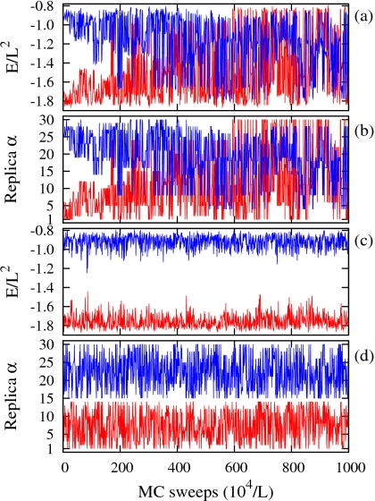
Actual replica trajectories initiated from α=1 and 30 in Figs. 4a, 4b start to sample the whole dynamic energy range after 3×10⁴ MCS and exhibit very frequent tunneling transitions in both energy and replica spaces via the localized GPDFs across the transition region. For comparison we also performed a tREM simulation with M=30, employing an equidistant temperature allocation for the same temperature range between T₁ and T_M. Two effectively disjointed sampling domains with no replica exchanges around α=14 are apparent in Figs. 4c, 4d due to a vanishing energy overlap between far-separated energy distributions of neighboring replicas at T_c.

Figure 4.

Simulated trajectories of α=1 and 30 in (a) energy and (b) replica space of the gREM₃, and in (c) energy and (d) replica space of the tREM for Potts spins with L=64.

γ₀ dependence of the gREM

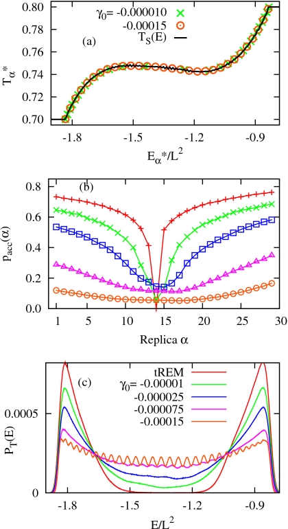
Varying γ₀ directly affects the gREM simulation by changing the width of GPDFs and the distribution of $E_{\alpha }^{*}$. These effects are entangled in Eq. 8 since decreasing γ₀ produces a more dense population of $E_{\alpha }^{*}$ for the transition region, as demonstrated in Fig. 5a, but a narrower GPDF in each replica due to the increased ${\sigma }_{\gamma }=T_{\alpha }^{*2}∕\left({\gamma }_S-{\gamma }_0\right)$. The collapse of $\left[E_{\alpha }^{*},T_{\alpha }^{*}\right]$ of both gREM₁ and gREM₄ into T_S(E) determined by STMC reveals that the most probable energy set indeed traces a locus of T_S(E).

Figure 5.

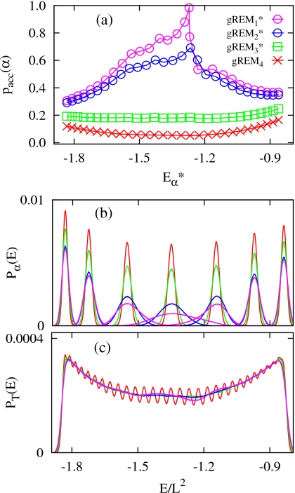
(a) Most probable energy set $\left[E_{\alpha }^{*},T_{\alpha }^{*}\right]$ of the gREM₁ and the gREM₄ simulations, (b) acceptances probabilities p_acc(α), and (c) superimposed energy distributions P_T(E) of various gREM simulations in Table 1 with varying γ₀ for fixed L=64. Same colors are used for the same simulations in both (b) and (c).

Due to the opposing effects of γ₀ for energy overlaps between neighboring replicas, the acceptance probability, p_acc(α), for replica exchanges between α and (α+1) shows a nonmonotonic γ₀-dependence in Fig. 5b. The tREM shows no replica exchanges around T_c≈0.745 46, with a minimum in p_acc(α) at α=14 (T₁₄=0.7448 and T₁₅=0.7482). On the other hand, a systematic enhancement of p_acc(α) shows up around α=14 in the gREM as the effective temperatures form stable crossing points in the transition region, upon decreasing γ₀ to −0.000 025. A further decrease to γ₀=−0.000 15 yields an almost uniform acceptance, but an overall reduction in p_acc(α) due to significantly narrowed GPDFs.

The γ₀-dependence of the gREM is also clearly captured in the superimposed energy distributions, P_T(E), in Fig. 5c, illustrating that phase-coexistent energy states between −1.5L² and −1.1L² are only accessible for ${\gamma }_0<{\gamma }_S^{\text{min}}\approx -0.000005$. The existence of the threshold value ${\gamma }_S^{\text{min}}$ reveals that the success of the gREM relies on the transformation of unstable energy states of canonical ensembles into stable ones with optimized noncanonical ensembles. As steeper effective temperatures produce a denser population of $E_{\alpha }^{*}$ in the transition region, P_T(E) becomes more flattened for the entire energy range, with characteristic oscillatory structures, stemming from sharply peaked P_α(E) as in the gREM₄.

Forming more stable crossing points, $E_{\alpha }^{*}$, in the transition region is crucial for sampling phase-coexistent states and smoothly joining ordered and disordered phases in the gREM. However, narrowed GPDFs with decreasing γ₀ is not desirable for p_acc(α), as shown in Fig. 5a. To resolve this problem we performed additional simulations, denoted by the gREM^* in Table 1, employing new effective temperatures as

$$T_{\alpha }^{*}\left(E;{\lambda }_{\alpha }^{*}\right)={\lambda }_{\alpha }^{*}+{\gamma }_0\left(E-E_0\right)=T_{\alpha }^{*}+{\gamma }_0\left(E-E_{\alpha }^{*}\right),$$ (13)

with ${\lambda }_{\alpha }^{*}=T_{\alpha }^{*}-{\gamma }_0\left(E_{\alpha }^{*}-E_0\right)$. In Eq. 13, newly assigned control parameters ${\lambda }_{\alpha }^{*}$ make $T_{\alpha }^{*}\left(E;{\lambda }_{\alpha }^{*}\right)$ cross the most probable energy set $\left[E_{\alpha }^{*},T_{\alpha }^{*}\right]$ of the gREM₄, maintaining a dense population of $E_{\alpha }^{*}$ for the transition region irrespective of γ₀.

As seen in Fig. 6a, a significant enhancement of p_acc(α), with an overall uniform acceptance, is obtained for $g{\text{REM}}_3^{*}$, in comparison with gREM₃, even with the same γ₀=−0.000 075. The increase in p_acc(α) for the transition region is more dramatic with a lower γ₀, as in $g{\text{REM}}_1^{*}$ and $g{\text{REM}}_2^{*}$, corresponding to γ₀=−0.000 007 5 and −0.000 015, respectively. The systematic increase in p_acc(α) is mainly due to more delocalized GPDFs in the gREM^* simulations with increasing γ₀, while maintaining centers of Gaussians at nearly the same $E_{\alpha }^{*}$, as illustrated in Fig. 6b. More delocalized energy distributions maximize energy overlaps among replicas, leading to a significant acceleration of replica exchanges. As a result, the uniform energy sampling in P_T(E) remains unchanged in Fig. 6c regardless of γ₀ and oscillatory structures are smoothed out. This implies that an optimal performance of the gREM is achieved by first determining densely populated $\left[E_{\alpha }^{*},T_{\alpha }^{*}\right]$ with a steeper γ₀ and then switching to a production run with Eq. 13 at ${\gamma }_0\simeq {\gamma }_S^{\text{min}}$.

Figure 6.

(a) p_acc(α) as a function of $E_{\alpha }^{*}$, (b) resulting GPDFs, and (c) superimposed P_T(E) of the gREM^* simulations in Table 1 for L=64. In (b), α=1, 5, 10, 15, 20, 25, and 30 from left to right.

Accelerated tunneling transitions

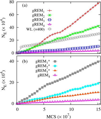
To systematically quantify the performance of the gREM simulations we compute the number of tunneling transitions in energy, denoted by N_E, measuring how often all replicas make transitions from one phase to the other.^{25, 47, 53, 57, 58} We also calculate the mean tunneling time, τ_E, by determining the inverse of a linear slope of N_E in production phases of the gREM simulations. Tunneling transitions were counted between the two boundary energies of −1.80L² and −0.85L².

Except for an equilibration stage, N_E in Fig. 7a is linearly increasing as a function of the total simulation time. This implies that barrier crossing rates, which are proportional to the slope of N_E, are almost constant throughout the simulations. The most frequent tunneling transitions were observed in gREM₁ with γ₀=−0.000 01, and N_E systematically decreases as γ₀ decreases from ${\gamma }_S^{\text{min}}$, even with a more comprehensive sampling and a better p_acc(α) for the phase transition region in Figs. 5a, 5b.

Figure 7.

Accumulated tunneling transitions: N_E as a function of a total MCS in (a) the gREM and (b) the gREM^* simulations in Table 1 for L=64. In (a), N_E of the WL has been magnified by 400 times for visualization and the gREM^* simulations in (b) were performed with $T_{\alpha }^{*}\left(E;{\lambda }_{\alpha }^{*}\right)$ based on $\left[E_{\alpha }^{*},T_{\alpha }^{*}\right]$ of the gREM₄.

The attenuation of N_E with decreasing γ₀ is mainly due to the increased number of intermediate replicas in the transition region, causing tunneling to require more consecutive replica exchanges. On the other hand, tunneling in the gREM with γ₀ close to ${\gamma }_S^{\text{min}}$ is rather rapid since a couple of replica exchanges among sparsely distributed intermediate replicas leads to a tunneling even with a relatively poor p_acc(α). However, the accelerated N_E with ${\gamma }_0\approx {\gamma }_S^{\text{min}}$ does not necessarily lead to an enhanced convergence because the transition region is poorly sampled due to a lack of replicas, as seen in P_T(E) of Fig. 5c.

The effect of γ₀ on N_E is more apparent in the gREM^* simulations in Fig. 7b, in which the location of intermediate replicas around the transitions region is almost frozen. As expected, increasing γ₀, yielding more delocalized GPDFs centered at the same $E_{\alpha }^{*}$ of the gREM₄, results in a monotonic acceleration of N_E, while retaining a faithful sampling in the transition region even with γ₀ close to ${\gamma }_S^{\text{min}}$. Approximately a tenfold speedup of N_E is observed in $g{\text{REM}}_1^{*}$ compared to gREM₄.

For a comparison we also performed the entropic version of the WL sampling⁴⁸ for the energy range between −1.83L² and −0.83L². The entropy estimate $\tilde{S}\left(E\right)$ has been refined up to f_d=f−1=10⁻⁹, employing the dynamic update scheme $\tilde{S}\left(E\right)=\tilde{S}\left(E\right)+\text{ln\hspace{0.17em}}f$. Following the original convention, the modification factor was reduced to f once $\left|H\left(E\right)-\overline{H}\right|∕\overline{H}\le 0.2$, starting from 1.01, with $\overline{H}$ being the average energy histogram. Tunneling transitions in Fig. 7a, which has been magnified 400 times for visualization, show a steep rise at the initial stage of simulation, in which the nonvanishing modification factor ln f constantly biases the system to move away from visited energy regions. The reduction in f is very rapid initially, and f_d reaches 10⁻⁶ after 3.3×10⁷ MCS, but significantly slows down as f_d becomes smaller, resulting in a total of 1.5×10⁸ MCS up to f_d=10⁻⁹.

The most remarkable point in Fig. 7a is the dramatic acceleration of N_E in the gREM simulations over the WL. Examining the τ_E, in Table 1, reveals a speedup of tunneling transitions in the poorest case of our algorithm (gREM₄) of almost 60 times, increasing up to about 150 times for gREM₃. The acceleration of N_E is more significant for the gREM^* simulations, in which replicas are more densely populated for the backbending region regardless of γ₀ with Eq. 13. The ratio of tunneling times, $R_{\tau }={\tau }_E^{\text{WL}}∕{\tau }_E^{g\text{REM}}$, is about 600 in the $g{\text{REM}}_1^{*}$. Here we only considered the simulations having a comprehensive sampling for the transition region, as in WL sampling.

What is the underlying mechanism for an order of magnitude acceleration of N_E in the gREM over the WL? The bottleneck of barrier crossings in Potts spins is the formation of phase-coexistent states with interfacial regions, which becomes exponentially suppressed in the canonical ensemble. Flat histogram methods such as the multicanonical (MUCA) sampling,⁴⁷ WL,⁴⁸ and STMC (Ref. ⁴⁹) alleviate this exponential slowing down by enhancing mixed-phase configurations, employing a sampling weight inversely proportional to the density of states. However, in a single replica simulation of the flat histogram type, forming mixed-phase configurations starting from ordered or disordered phases is intrinsically sequential and cumulative, and τ_E is mainly limited by the diffusion rate in energy space.

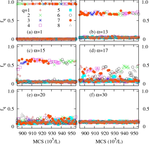
On the other hand, some intermediate replicas located at the transition region in the gREM always retain phase-coexistent states and naturally bridge the ordered and disordered phases through replica exchanges, as illustrated in Figs. 8a, 8b, 8c, 8d, 8e, 8f, in which fractions of spin states, f_q=∑_iδ(S_i,q)∕L², in the gREM₃, were plotted as a function of MCS for different α. In the ordered phase (α=1), most spins occupy a single spin state, while all spin states are equally probable in the disordered phase (α=30). Intermediate replicas of α=13, 15, and 17 exclusively sample mixed-phase configurations characterized by a majority state with f_q>0.5 and other states with f_q≈0; these mixed-phase states are preserved throughout the simulation. We conclude that the main limiting factor for tunneling in the gREM is the efficacy of replica exchanges among intermediate replicas sampling phase-coexistent states.

Figure 8.

Time profiles of f_q=∑_iδ(S_i,q)∕L² in the gREM₃ in Table 1 for L=64. Notice that intermediate replicas of α=13, 15, and 17 exclusively sample mixed-phase configurations consist of a major spin state with f_q>0 and other minor spin states with f_q≈0.

Scaling behavior of τ_E and T_S(E)

In a completely unbiased random walk in energy, corresponding to an ideal limit of flat histogram methods, τ_E scales as L^2d, with d being the dimension of the system (d=2 in this paper), since the dynamic energy range expands as L^d. In an actual simulation, τ_E scales like L^2d+z due to a deviation from a perfect random walk.^{47, 57} The value of z depends on the system and is known to be 0.65 for Potts spins and 0.73 for Ising spins, from studies using the MUCA (Ref. ⁴⁷) and the flat histogram sampling exploiting the exact S(E),⁵⁷ respectively.

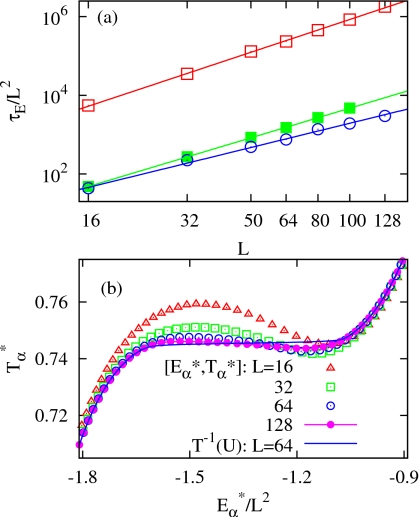
As summarized in Table 2, we performed several WL simulations, varying L from 16 to 128. The dynamic energy range was restricted between $E_1^{*}$ and $E_M^{*}$ determined by the gREM simulation at the same L. A similar scaling behavior ${\tau }_E^{\text{WL}}\simeq 2.44\times L^{2d+0.77}$ appears in the WL simulation for Potts spins, as seen in Fig. 9a, in which the log-log plot of τ_E and L shows a clear linear relationship. A slightly larger exponent of z=0.77, in comparison with that of the MUCA,⁴⁷ might be due to the difference in energy boundaries for tunneling. In our study, transitions were counted between $E_1^{*}$ and $E_M^{*}$, but tunneling transitions in the MUCA were counted between two free energy maxima at T_c, which have a much smaller separation.

Table 2.

Mean tunneling times τ_E and simulations times t_S of the WL simulations with varying L. Entropy estimates were refined up to f_d=10⁻⁹.

L	16	32	50	64	80	100	128
τE (×105) (MCS)	0.055	0.35	1.31	2.34	4.52	8.44	18.12
tS (×107) (MCS)	0.98	3.16	7.47	1.51	1.69	24.5	32.2

Figure 9.

(a) Log-log plots of mean tunneling times τ_E and L for the WL, and the gREM^I and the gREM^II simulations from top to bottom, and (b) profiles of T_S(E) estimated by $\left[E_{\alpha }^{*},T_{\alpha }^{*}\right]$ of the gREM^II simulations with varying L. In (a), lines are linear fits to the corresponding data points.

To examine scaling properties of the gREM we performed two different sets of simulations with varying L, as summarized in Table 3. Simulations in set I denoted by gREM^I are associated with the effective temperature of Eq. 8 with M=30 at the fixed ${\gamma }_0^{\text{I}}=-0.000075$. Set II denoted by the gREM^II was performed with the scaled${\gamma }_0^{\text{II}}=-0.000075\times {\left(64∕L\right)}^2$ and M=50. Since the backbending region in T_S(E) becomes flat with increasing L [see Fig. 9b], ${\gamma }_0^{\text{II}}$ in the gREM^II is systematically lowered by the scaling factor (64∕L)², producing more delocalized GPDFs and enhancing p_acc(α) for the transition region. Since the simulation with L=128 in the gREM^I did not show statistically meaningful transitions, it was excluded in the scaling analysis.

Table 3.

Simulation parameters and mean tunneling times τ_E for the gREM^I and gREM^II simulations with varying L. The gREM^I simulations are associated with ${\gamma }_0^{\text{I}}=-0.000075$ and M=30. The $g{\text{REM}}_7^{*}$ was performed with Eq. 13 based on $\left[E_{\alpha }^{*},T_{\alpha }^{*}\right]$ of the gREM₇. ${\tau }_E^{\text{I}}$ and ${\tau }_E^{\text{II}}$ correspond to the gREM^I and gREM^II, respectively.

Methods	L	${\gamma }_0^{\text{II}}\left(M=50\right)$	${\tau }_E^{\text{I}}$ (MCS)	${\tau }_E^{\text{II}}$ (MCS)	tS (MCS)
gREM1	16	−0.0012	48.1	43.7	1.0×107
gREM2	32	−0.0003	274.7	224.2	7.0×107
gREM3	50	−0.00012	851.0	487.1	1.5×108
gREM4	64	−0.000075	1511.7	755.3	1.5×108
gREM5	80	−0.000048	2710.2	1371.1	1.5×108
gREM6	100	−0.000031	4739.1	1920.2	1.5×108
gREM7	128	−0.0000187		2998.3	1.5×108
$g{\text{REM}}_7^{*}$	128	−0.0000038		139.5	1.5×108

The comparison of τ_E in Table 3 reveals that the speedup in N_E with increasing L is even more remarkable in both gREM^I and gREM^II. The ratio $R_{\tau }={\tau }_E^{\text{WL}}∕{\tau }_E^{g\text{REM}}$ increases from about 10² order at L=32 to 10⁴ order at L=128. An apparent linear behavior in the log-log plot of L and τ_E is seen in the gREM^I of Fig. 9a. The scaling behavior follows ${\tau }_E^{\text{I}}\simeq 0.047\times L^{2d+0.5}$, implying that the acceleration of N_E in the gREM^I is about 10² order up to L=100. When more crossing points are created in the phase transition region with M=50, the growth of τ_E as a function of L is weaker, with a lower slope in the log-log plot in the gREM^II, yielding ${\tau }_E^{\text{II}}\simeq 0.156\times L^{2d+0.0477}$. The scaling behavior of the gREM approaches that of a random walk in energy as more replicas are built up in the phase transition region.⁵⁷

The profiles of T_S(E) represented by the most probable energy set $\left[E_{\alpha }^{*},T_{\alpha }^{*}\right]$ show a clear backbending for L=16 and 32 in Fig. 9b, but the extent of the backbending gradually declines with increasing L and becomes almost flat at L=128. In contrast to the backbending in the microcanonical caloric curve, T_S(E), the inverse of the internal energy, T=U⁻¹(E), which corresponds to a caloric curve in the canonical ensemble, monotonically increases across the phase transition region, implying that statistical ensembles are not equivalent in finite size systems.^{29, 30}

Thermodynamics

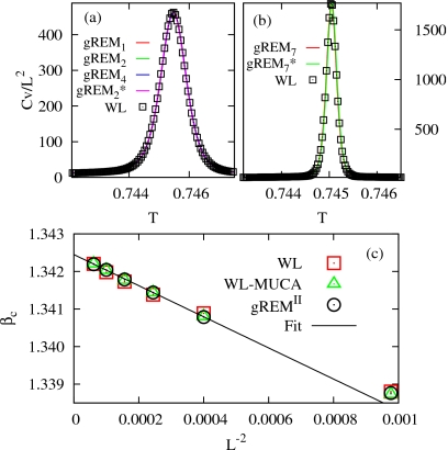
After a sufficient long production run the gREM determines the entropy estimate, $\tilde{S}\left(E\right)$, by joining multiple replica simulations via the WHAM.⁵⁵ Once $\tilde{S}\left(E\right)$ is determined, all canonical thermodynamic properties, such as the internal energy, U(T), and the heat capacity, C_v(T), are completely determined. As demonstrated in Fig. 10a, heat capacities (lines) determined by various gREM simulations in Table 1 for L=64 are collapsed into a single curve with good agreement with the WL-MUCA simulation (squares), irrespective of simulation conditions. Also, heat capacities at L=128 in Fig. 10b determined by both gREM₇ and $g{\text{REM}}_7^{*}$ in Table 2 are almost indistinguishable from that of the WL-MUCA even with a significantly shorter simulation time.

Figure 10.

Heat capacities C_v(T) around T_c of the WL-MUCA and various gREM simulations for Potts spins at (a) L=64 and (b) L=128, and plots of β_c(L) with L⁻² for the gREM^II in Table 3, the WL, and the WL-MUCA simulations. In (b), the line is a linear fit to the data of the gREM^II.

Here WL-MUCA denotes the MUCA sampling with the frozen $\tilde{S}\left(E\right)$ refined by the WL up to f_d=10⁻⁹. We found that thermodynamic properties determined by a bare $\tilde{S}\left(E\right)$ gives a systematic discrepancy from those of the gREM simulations, as demonstrated in the plot of β_c with L⁻² in Fig. 10b. Indeed, it is found that energy distributions P_MU(E) obtained by the MUCA sampling with the frozen $\tilde{S}\left(E\right)$ for 10⁸ MCS show a considerable deviation from a uniform sampling, implying that the WL $\tilde{S}\left(E\right)$ still contains an error stemming from the refinement process.⁵⁹ We correct this error by applying the reweighting process for the entropy estimate as ${\tilde{S}}_{\text{MU}}\left(E\right)=\tilde{S}\left(E\right)+\text{ln\hspace{0.17em}}{P}_{\text{MU}}\left(E\right)$. As shown in Figs. 10a, 10b the reweighted ${\tilde{S}}_{\text{MU}}\left(E\right)$ produce thermodynamics consistent with that of the gREM.

At finite L the singularities and discontinuities in first-order phase transitions of infinite systems are smeared out,⁶⁰ and backbending emerges in T_S(E). With increasing L, T_S(E) becomes flat, rounded transitions transform into sharp ones, and the size dependent critical temperature, β_c(L)=1∕T_c(L), approaches the thermodynamic transition temperature, ${\beta }_c^{\infty }=1∕T_c^{\infty }$. This asymptotic behavior can be predicted by finite size scaling analysis⁶¹ as

$${\beta }_c\left(L\right)={\beta }_c^{\infty }+1∕L^d,$$ (14)

in which the critical temperature, β_c(L), was determined as the temperature at the peak in C_v(T).

As seen in Fig. 10b, the critical temperatures determined by the gREM^II and the WL-MUCA are in quantitative agreement. Furthermore, plotting β_c(L) versus L⁻² yields a good straight line, extrapolating to ${\beta }_c^{\infty }=1.332447$, close to the exact $\text{ln}\left(1+\sqrt{Q=8}\right)=1.342454$.⁵⁶ On the other hand, a noticeable deviation from a linear fit shows up in the scaling behavior of β_c(L) in the original WL. To eliminate finite size effects at a smaller L, we used the data set between L=50 and L=120 for a linear fit.

CONCLUSIONS

The generalized Replica Exchange Method (gREM) has been developed to facilitate effective configurational sampling in systems exhibiting backbending, or an S-loop, in the statistical temperature, T_S(E), characteristic of first-order phase transitions in finite systems. By combining optimally parametrized, generalized ensemble samplings with replica exchanges, our method enables a comprehensive sampling for phase transition regions with successive unimodal energy distributions, by transforming metastable or unstable energy states of canonical ensembles into stable ones. Exploiting the one-to-one correspondence between the sampling weight and the effective temperature, we also present an inverse mapping strategy, which determines optimal sampling weights from tailored effective temperatures, avoiding an intrinsic instability of the canonical ensemble to the negative slope region of T_S(E).

The effectiveness of our method has been explicitly demonstrated for Potts spin systems, for various simulations conditions, as a function of the system size, L. The quantitative comparison between the gREM and WL sampling reveals that the gREM provides an order of magnitude acceleration of tunneling transitions over the WL, while maintaining a faithful sampling for the phase transition region as in flat histogram methods. The underlying mechanism for accelerated tunneling transitions is the capacity of the gREM to preserve mixed-phase configurations in intermediate replicas located at the transition region. Finite size scaling analysis shows that in the optimum case of the gREM, the scaling of the mean tunneling time, τ_E, approaches ∝L^2d, corresponding to the ideal limit of flat histogram methods. It is also shown that the gREM provides a correct canonical thermodynamics via the reweighting with a much smaller simulation time.

Finally, we would like to emphasize that the inverse mapping strategy is a general framework that can be applied to the combination of any generalized ensemble sampling and the replica exchange method. We anticipate that a hybrid extension augmented by the inverse mapping, applying the gREM to selective transition regions while retaining the tREM for other energy regions, will allow the widespread use of our method to various systems with first-order transitions.

References

- Swendsen R. H. and Wang J. S., Phys. Rev. Lett. 57, 2607 (1986). 10.1103/PhysRevLett.57.2607 [DOI] [PubMed] [Google Scholar]
- Geyer C. J. and Thompson A., J. Am. Stat. Assoc. 90, 909 (1995). 10.2307/2291325 [DOI] [Google Scholar]
- Hukushima K. and Nemoto K., J. Phys. Soc. Jpn. 65, 1604 (1996). 10.1143/JPSJ.65.1604 [DOI] [Google Scholar]
- Hansmann U. H. E., Chem. Phys. Lett. 281, 140 (1997). 10.1016/S0009-2614(97)01198-6 [DOI] [Google Scholar]
- Sugita Y. and Okamoto Y., Chem. Phys. Lett. 314, 141 (1999). 10.1016/S0009-2614(99)01123-9 [DOI] [Google Scholar]
- Zhou R. and Berne B. J., Proc. Natl. Acad. Sci. U.S.A. 99, 12777 (2002) 10.1073/pnas.142430099 [DOI] [PMC free article] [PubMed] [Google Scholar]; Garcia A. E. and Onuchic J. N., Proc. Natl. Acad. Sci. U.S.A. 100, 13898 (2003). 10.1073/pnas.2335541100 [DOI] [PMC free article] [PubMed] [Google Scholar]
- Yamamoto R. and Kob W., Phys. Rev. E 61, 5473 (2000). 10.1103/PhysRevE.61.5473 [DOI] [PubMed] [Google Scholar]
- Frantsuzov P. A. and Mandelshtam V. A., Phys. Rev. E 72, 037102 (2005). 10.1103/PhysRevE.72.037102 [DOI] [PubMed] [Google Scholar]
- Newman M. E. J. and Barkema G. T., Monte Carlo Methods in Statistical Physics (Clarendon, Oxford, 1999). [Google Scholar]
- Sugita Y. and Okamoto Y., Chem. Phys. Lett. 329, 261 (2000) 10.1016/S0009-2614(00)00999-4 [DOI] [Google Scholar]; Mitsutake A., Sugita Y., and Okamoto Y., J. Chem. Phys. 118, 6664 (2003) 10.1063/1.1555847 [DOI] [Google Scholar]; Mitsutake A., Sugita Y., and Okamoto Y., J. Chem. Phys. 118, 6676 (2003). 10.1063/1.1555849 [DOI] [Google Scholar]
- Calvo F. and Doye J. P. K., Phys. Rev. E 63, 010902 (2000). 10.1103/PhysRevE.63.010902 [DOI] [Google Scholar]
- Faller R., Yan Q., and de Pablo J. J., J. Chem. Phys. 116, 5419 (2002). 10.1063/1.1456504 [DOI] [Google Scholar]
- Fukunishi H., Watanabe O., and Takada S., J. Chem. Phys. 116, 9058 (2002). 10.1063/1.1472510 [DOI] [Google Scholar]
- Whitfield T. W., Bu L., and Straub J. E., Physica A 305, 157 (2002). 10.1016/S0378-4371(01)00656-2 [DOI] [Google Scholar]
- Jang S., Shin S., and Park Y., Phys. Rev. Lett. 91, 058305 (2003). 10.1103/PhysRevLett.91.058305 [DOI] [PubMed] [Google Scholar]
- Liu P., Kim B., Friesner R. A., and Berne B. J., Proc. Natl. Acad. Sci. U.S.A. 102, 13749 (2005) 10.1073/pnas.0506346102 [DOI] [PMC free article] [PubMed] [Google Scholar]; Liu P., Huang X., Zhou R., and Berne B. J., J. Phys. Chem. B 110, 19018 (2006). 10.1021/jp060365r [DOI] [PMC free article] [PubMed] [Google Scholar]
- Cheng X., Cui G., Hornak V., and Simmering C., J. Phys. Chem. B 109, 8220 (2005). 10.1021/jp045437y [DOI] [PMC free article] [PubMed] [Google Scholar]
- Lyman E., Ytreberg F. M., and Zuckerman D. M., Phys. Rev. Lett. 96, 028105 (2006). 10.1103/PhysRevLett.96.028105 [DOI] [PubMed] [Google Scholar]
- Calvo F., J. Chem. Phys. 123, 124106 (2005). 10.1063/1.2036969 [DOI] [PubMed] [Google Scholar]
- Rick S. W., J. Chem. Phys. 126, 054102 (2007). 10.1063/1.2431807 [DOI] [PubMed] [Google Scholar]
- Liu P. and Voth G. A., J. Chem. Phys. 126, 045106 (2007). 10.1063/1.2408415 [DOI] [PubMed] [Google Scholar]
- Kamberaj H. and van der Vaart A., J. Chem. Phys. 127, 234102 (2007). 10.1063/1.2806930 [DOI] [PubMed] [Google Scholar]
- Brenner P., Sweet C. R., VonHandorf D., and Izaguirre J. A., J. Chem. Phys. 126, 074103 (2007). 10.1063/1.2436872 [DOI] [PubMed] [Google Scholar]
- Zhang C. and Ma J., Phys. Rev. E 76, 036708 (2007). 10.1103/PhysRevE.76.036708 [DOI] [PMC free article] [PubMed] [Google Scholar]
- Trebst S., Troyer M., and Hansmann U. H. E., J. Chem. Phys. 124, 174903 (2006). 10.1063/1.2186639 [DOI] [PubMed] [Google Scholar]
- Ballard A. J. and Jarzynski C., Proc. Natl. Acad. Sci. U.S.A. 106, 12224 (2009). 10.1073/pnas.0900406106 [DOI] [PMC free article] [PubMed] [Google Scholar]
- Kar P., Nadler W., and Hansmann U. H. E., Phys. Rev. E 80, 056703 (2009). 10.1103/PhysRevE.80.056703 [DOI] [PubMed] [Google Scholar]
- Earl D. J. and Deem M. W., Phys. Chem. Chem. Phys. 7, 3910 (2005). 10.1039/b509983h [DOI] [PubMed] [Google Scholar]
- Behringer H. and Pleimling M., Phys. Rev. E 74, 011108 (2006). 10.1103/PhysRevE.74.011108 [DOI] [PubMed] [Google Scholar]
- Gross D. H. E., Rep. Prog. Phys. 53, 605 (1990). 10.1088/0034-4885/53/5/003 [DOI] [Google Scholar]
- Lopez O., Lacroix D., and Vient E., Phys. Rev. Lett. 95, 242701 (2005). 10.1103/PhysRevLett.95.242701 [DOI] [PubMed] [Google Scholar]
- Junghans C., Bachmann M., and Janke W., Phys. Rev. Lett. 97, 218103 (2006). 10.1103/PhysRevLett.97.218103 [DOI] [PubMed] [Google Scholar]
- Hernández-Rojas H. and Gomez Llorente J. M., Phys. Rev. Lett. 100, 258104 (2008). 10.1103/PhysRevLett.100.258104 [DOI] [PubMed] [Google Scholar]
- Kim J., Keyes T., and Straub J. E., Phys. Rev. E 79, 030902(R) (2009). 10.1103/PhysRevE.79.030902 [DOI] [PMC free article] [PubMed] [Google Scholar]
- Labastie P. and Whetten R. L., Phys. Rev. Lett. 65, 1567 (1990). 10.1103/PhysRevLett.65.1567 [DOI] [PubMed] [Google Scholar]
- Wales D. J. and Berry R. S., Phys. Rev. Lett. 73, 2875 (1994). 10.1103/PhysRevLett.73.2875 [DOI] [PubMed] [Google Scholar]
- D’Agostino M., Gulminelli F., Chomaz Ph., Bruno M., Cannata F., Bougault R., Gramegna F., Iori I., Le Neindre N., Margagliotti G. V., Moroni A., and Vannini G., Phys. Lett. B 473, 219 (2000). 10.1016/S0370-2693(99)01486-0 [DOI] [Google Scholar]
- Schmidt M., Kusche R., Hippler T., Donges J., Kronmüller W., von Issendorff B., and Haberland H., Phys. Rev. Lett. 86, 1191 (2001). 10.1103/PhysRevLett.86.1191 [DOI] [PubMed] [Google Scholar]
- Huang K., Statistical Mechanics (Wiley, New York, 1972). [Google Scholar]
- Challa M. S. S. and Hetherington J. H., Phys. Rev. Lett. 60, 77 (1988). 10.1103/PhysRevLett.60.77 [DOI] [PubMed] [Google Scholar]
- Neuhaus T., Magiera M. P., and Hansmann U. H. E., Phys. Rev. E 76, 045701(R) (2007). 10.1103/PhysRevE.76.045701 [DOI] [PubMed] [Google Scholar]
- Kim J., Fukunishi Y., and Nakamura H., Phys. Rev. E 67, 011105 (2003). 10.1103/PhysRevE.67.011105 [DOI] [PubMed] [Google Scholar]
- Kim J., Fukunishi Y., Kidera A., and Nakamura H., Phys. Rev. E 68, 021115 (2003). [DOI] [PubMed] [Google Scholar]
- Heinsalu E., Tammelo R., and Örd T., Phys. Rev. E 69, 021111 (2004). 10.1103/PhysRevE.69.021111 [DOI] [PubMed] [Google Scholar]
- Kim J., Fukunishi Y., and Nakamura H., J. Chem. Phys. 121, 1626 (2004). 10.1063/1.1763841 [DOI] [PubMed] [Google Scholar]
- Kim J., Fukunishi Y., Kidera A., and Nakamura H., J. Chem. Phys. 121, 5590 (2004). 10.1063/1.1786578 [DOI] [PubMed] [Google Scholar]
- Berg B. A. and Celik T., Phys. Rev. Lett. 69, 2292 (1992) 10.1103/PhysRevLett.69.2292 [DOI] [PubMed] [Google Scholar]; Berg B. A. and Celik T., Phys. Lett. B 267, 249 (1991). 10.1016/0370-2693(91)91256-U [DOI] [Google Scholar]
- Wang F. and Landau D. P., Phys. Rev. Lett. 86, 2050 (2001) 10.1103/PhysRevLett.86.2050 [DOI] [PubMed] [Google Scholar]; Wang F. and Landau D. P., Phys. Rev. E 64, 056101 (2001). 10.1103/PhysRevE.64.056101 [DOI] [PubMed] [Google Scholar]
- Kim J., Straub J. E., and Keyes T., Phys. Rev. Lett. 97, 050601 (2006) 10.1103/PhysRevLett.97.050601 [DOI] [PubMed] [Google Scholar]; Kim J., Straub J. E., and Keyes T., J. Chem. Phys. 126, 135101 (2007) 10.1063/1.2711812 [DOI] [PubMed] [Google Scholar]; Kim J., Straub J. E., and Keyes T., Phys. Rev. E 76, 011913 (2007). 10.1103/PhysRevE.76.011913 [DOI] [PubMed] [Google Scholar]
- Tsallis C., J. Stat. Phys. 52, 479 (1988). 10.1007/BF01016429 [DOI] [Google Scholar]
- Andricioaei I. and Straub J. E., Phys. Rev. E 53, R3055 (1996). 10.1103/PhysRevE.53.R3055 [DOI] [PubMed] [Google Scholar]
- Andricioaei I. and Straub J. E., J. Chem. Phys. 107, 9117 (1997). 10.1063/1.475203 [DOI] [Google Scholar]
- Kim J. and Straub J. E., J. Chem. Phys. 130, 144114 (2009). 10.1063/1.3108523 [DOI] [PMC free article] [PubMed] [Google Scholar]
- Hansmann U. H. E. and Okamoto Y., Phys. Rev. E 56, 2228 (1997). 10.1103/PhysRevE.56.2228 [DOI] [Google Scholar]
- Ferrenberg A. M. and Swendsen R. H., Phys. Rev. Lett. 63, 1195 (1989). 10.1103/PhysRevLett.63.1195 [DOI] [PubMed] [Google Scholar]
- Wu F. Y., Rev. Mod. Phys. 54, 235 (1982) 10.1103/RevModPhys.54.235 [DOI] [Google Scholar]; Wu F. Y., Rev. Mod. Phys. 55, 315(E) (1983). 10.1103/RevModPhys.55.315 [DOI] [Google Scholar]
- Dayal P., Trebst S., Wessel S., Wurtz D., Troyer M., Sabhapandit S., and Coppersmith S. N., Phys. Rev. Lett. 92, 097201 (2004). 10.1103/PhysRevLett.92.097201 [DOI] [PubMed] [Google Scholar]
- Kim J., Keyes T., and Straub J. E., J. Chem. Phys. 130, 124112 (2009). 10.1063/1.3095422 [DOI] [PMC free article] [PubMed] [Google Scholar]
- Zhou C. and Su J., Phys. Rev. E 78, 046705 (2008). 10.1103/PhysRevE.78.046705 [DOI] [PubMed] [Google Scholar]
- Binder K. and Landau D. P., Phys. Rev. B 30, 1477 (1984). 10.1103/PhysRevB.30.1477 [DOI] [Google Scholar]
- Bazavov A., Berg B. A., and Dubey S., Nucl. Phys. B 802, 421 (2008). 10.1016/j.nuclphysb.2008.04.020 [DOI] [Google Scholar]