The Intrinsic Signal-to-Noise Ratio in Human Cardiac Imaging at 1.5, 3, and 4 T

Abstract

Cardiac imaging is inherently demanding on the signal-to-noise performance of the MR scanner and may benefit from high field strengths. However, the complex behavior of the radiofrequency field in the human body at high frequencies makes model-based analyses difficult. This study aims to obtain reliable comparisons of the signal-to-noise profile in the human chest in vivo at 1.5, 3, and 4 T. By using an RF-field-mapping method, it is shown that the intrinsic signal-to-noise increases with the field strength up to 4 T with a less than linear relation. The RF field profile is markedly distorted at 4 T, and the onset of this distortion is dependent on the body size. The high power deposition and the consequences of the RF field distortion are discussed.

INTRODUCTION

Cardiac imaging often requires high temporal and spatial resolution in order to acquire critical functional information. These requirements make extraordinary demands on the signal-to-noise ratio (SNR) in cardiac MRI. A significant determinant of the SNR is the static magnetic field strength (1, 2). However, there are only a few comparison studies of the signal-to-noise ratio in the human torso at different field strengths (3–5), especially in the chest. Most previous work has been with models or phantoms using a varying degree of complexity.

There are several problems with using analytical or numerical models or phantom measurements for determining the field dependence of SNR in humans. Most models and phantoms have too simple a geometry and composition to sufficiently describe the body. This is due to the complex and variable three-dimensional structure of the body, the uncertainty in the electrodynamic properties of tissues in the radiofrequency range, and its heterogeneous composition. In addition, most 3D models have used the quasi-static approximation, which ignores the induced field from the conductive and dielectric currents in the body. However, at high field strengths, the RF wavelength and the RF penetration depth approach the dimension of the body, resulting in a significant contribution of the induced conductive and dielectric currents and phase variation of the RF field across the body. Under these conditions, the quasi-static approximation needs to be replaced with the full Maxwell equations. This point was illustrated by phase-sensitive electric field measurements up to 110 MHz in elliptical phantoms in the context of hyperthermia (6, 7), and by measurements of the power deposition (8) and loading effect of the body on whole-body RF coils at frequencies up to 85 MHz (9), as well as loading effects of surface coils up to 100 MHz (10). Head images collected at 4 T also showed substantial dielectric resonant effects (11, 12). Rigorous analytical models of surface coil excitation (13, 14) and uniform volume excitation (15–17) of geometric samples also showed that the B₁ and heat-absorption distribution in the samples are greatly affected by the penetration and dielectric effects at high frequencies. Finite-element simulations of simplified body models suggest significant deviation of the B₁ distribution from the Biot–Savart law at high frequencies. This was demonstrated in surface coils loaded with spherical (18) or semiinfinite phantoms (19) and 3D heterogeneous models under uniform RF excitation (20). Despite the qualitative agreement between finite-element simulations and experimental observations, anatomically accurate models of the body are still too time consuming to compute with current computers without the quasi-static approximation.

With the existing limitation in numerical simulations, a direct experimental measure of the signal-to-noise ratio would be desirable. A convenient measure for experimentally comparing different field strengths is the intrinsic signal-to-noise ratio (ISNR). The ISNR was introduced by Edelstein et al. (3) and represents the signal-to-noise ratio in the absence of spin relaxation, field inhomogeneity effects, and motion and flow artifacts, as well as scanner hardware noise, etc. ISNR is purely determined by the electrodynamics at different field strengths and provides a basis for meaningful comparisons of the SNR independent of many parameters which are difficult to control or quantify. It is recognized however that ISNR is one of the many factors in the larger issue of overall cardiac imaging performance and serves as a starting point when considering the advantages and drawbacks of high field strength.

To derive the ISNR from images, the reciprocity relation is used (21). This relation states that (22)

$$\text{ISNR}(x,y,z)\propto B_0^2/\sqrt{P_{\text{e}}(x,y,z)},$$ [1]

where ISNR(x, y, z) is the ISNR at a location (x, y, z) in the body, B₀ is the static field strength, and P_e(x, y, z) is the power needed to generate a unit B₁, field at that location if the receive coil is used as a transmit coil. The constant of proportionality is strictly geometry- and B₀-independent (23), making this relation useful for human studies. The power coefficient P_e throughout the volume of interest can be obtained by mapping the magnitude of the B₁, field generated in the body with a known power input into the coil. If a field B₁(x, y, z) is generated with a power input P, then

$$P_{\text{e}}(x,y,z)=P/B_1{(x,y,z)}^2.$$ [2]

Equations [1] and [2] enable the measurement of ISNR with RF-field-mapping experiments.

Since surface coils are most common for signal reception in cardiac imaging, their ISNR and B₁ distributions were studied. The popular phased-array receive coil design consisting of several mutually isolated surface coils is dependent on the B₁ distribution of each element coil for the mutual isolation and overall optimization. Single-coil B₁ map information has implications regarding this design, as well as phased-array transmit designs at high fields. The purpose of this study was to measure the B₁, field distribution and ISNR for human cardiac imaging at 1.5, 3, and 4 T, to establish the dependence of these parameters on the static magnetic field strength.

MATERIAL AND METHODS

The studies were conducted at 1.5, 3, and 4 T. The 1.5 and 4 T studies were done at the National Institutes of Health on GE Signa platforms. The 3 T study was conducted at the University of Pittsburgh Medical College, also on a GE Signa platform. The method used for B₁, field mapping in vivo was a gradient-echo variant of the ratio method proposed by Stollberger et al. (24). Two sets of multislice images were acquired. One set was collected with a non-slice-selective, partially saturating, RF prepulse, which encoded the B₁, magnitude into the signal amplitude of the image. A control set of images was acquired without the prepulse to serve as an amplitude reference. The pulse sequence is shown in Fig. 1. The prepulse was a volumetric one-lobe sine pulse depicted in the figure, with a bandwidth of 3.3 kHz. This ratio-based method and the large bandwidth of the prepulse were chosen to minimize artifacts related to shim, motion and flow, and slice-profile imperfections (22, 23). The two sets of multislice images were collected by interleaving both the slices and the control/prepulse image sets. The data collection was gated to the EKG of the volunteers. The volunteers were trained to synchronize their breathing with the scans to reduce respiratory motion artifacts. For all field strengths the pulse sequence parameters were FOV = 400 mm (left to right) × 300 mm (anterior to posterior), matrix = 256 × 128, four slices of 5 mm thickness, TE = 6.7 ms, and TR = 3 s.

FIG. 1.

The pulse sequence used to map the B₁ field of surface coils in the chest. The ratio between the partially saturated image and the reference image yields the B₁ magnitude.

For the ISNR studies at 1.5, 3, and 4 T, two male volunteers were scanned. Volunteer 1 was 24 years old, 184 cm tall, and weighed 104 kg; volunteer 2 was 31 years old, 172 cm tall, and weighed 68 kg. They were chosen to represent a reasonable range of body sizes.

Surface coils with distributed capacitances were used for all field strengths. The geometries of all coils were the same, with 22.9 cm diameter. To account for the power dissipated in the coils, the loaded and unloaded Q of the coils were measured, and an efficiency factor was calculated (26),

$$\text{efficiency}=\frac{1/Q_{\text{loaded}}-1/Q_{\text{unloaded}}}{1/Q_{\text{loaded}}}.$$ [3]

This efficiency factor was multiplied with the RF amplifier output to give the power input P in Eq. [2].

To verify the lack of influence of B₀ inhomogeneity, which is significant at 3 and 4 T, a separate experiment was conducted at 4 T. Two B₁ field maps of a spherical phantom were collected with a surface coil, using the method outlined above. One map was collected with on-resonance RF excitation, and the other 200 Hz off resonance. The B₁, maps are shown in Fig. 2. The off-resonance effect was negligible.

FIG. 2.

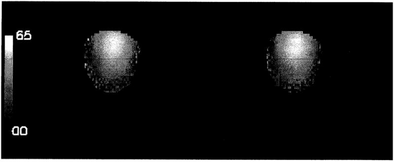
The B₁ maps of a spherical water phantom with a surface coil placed above it, collected at 4 T. The gray scale is in flip angles, from 0° to 65°. The map on the left was collected with the RF frequency on resonance; the map on the right was collected with the RF frequency off resonance by 200 Hz to simulate a bad shim condition.

The repetition time of the B₁ mapping sequence was three seconds. In order to rule out a driven equilibrium effect on the B₁ maps resulting from an incomplete spin recovery during this time, B₁ maps were collected with TR = 3 s and TR = 5 s on volunteer 2. This study was performed at 4 T since the water T₁, values are the longest, and therefore, the measurement is more sensitive to the 3 s TR. As shown in Fig. 3, the field maps of the different TR values were similar, suggesting that the driven equilibrium effect was negligible.

FIG. 3.

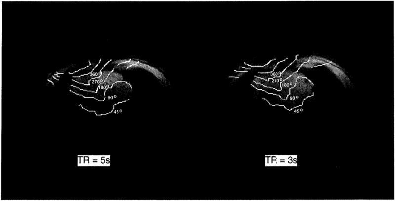
The B₁ maps of a transaxial slice of volunteer 2 at 4 T, collected with TR = 3 s and TR = 5 s, respectively. The flip-angle contours are overlaid on the reference images.

RESULTS

The B₁ field maps of each volunteer at 1.5, 3, and 4 T are presented in Fig. 4. For each volunteer one of the four transaxial slices is shown. Each image is a contour plot of the B₁ magnitude represented in spin-flip angles, overlaid on the reference images. In collecting these images, the power input into the coils was adjusted with a series of scout scans such that the flip angle at the center of the heart was 90° for all field strengths (see Table 1). The field pattern distortion and left–right asymmetry increased from 1.5 to 4 T. The left–right asymmetry is partially due to the fact that the MR-sensitive component of the B₁, field is one of the two circularly polarized components of the actual RF magnetic field (28). At 1.5 T, this asymmetry was already visible.

FIG. 4.

Radiofrequency field maps of transaxial slices of volunteers 1 and 2 at 1.5, 3, and 4 T. The B₁ distribution is represented as flip-angle contours overlaid on reference images which were used for the B₁ calculations. In the B₁ mapping experiments, the power input into the surface coils was adjusted such that the flip angle at the center of the heart was 90°.

TABLE 1.

A Summary of the ISNR at the Center of the Heart at 1.5, 3, and 4 T in Two Volunteers

	Volunteer 1			Volunteer 2
Height and weight	184 cm, 104 kg			172 cm, 68 kg
Field strength (T)	1.5	3	4	1.5	3	4
Pe (kW)	0.149	0.62	1.34	0.120	0.592	1.09
Coil efficiency (%)	79	84	89	81	87	91
Relative ISNR	1	1.66	2.36	1	1.80	2.36

Note. The parameter P_e is the power needed to generate a 1 ms 90° pulse at the center of the heart. The coil efficiency was calculated from the loaded and unloaded Q measurements (Eq. [3]). The relative ISNR numbers are normalized to 1.5 T.

The field-penetration profiles along a line from the anterior chest wall toward the heart were plotted for both volunteers in Figs. 5a and 5b. The RF field gradient generally increased with the main field strength. For volunteer 1, of larger chest size, the decrease in penetration depth was evident between 1.5 and 3 T. For volunteer 2, of smaller chest size, the greatest decrease in penetration depth occurred between 3 and 4 T. The difference in the onset of the large penetration depth change is likely caused by different chest sizes. For a smaller chest size, the RF wavelength approaches the dimension of the chest at higher frequencies.

FIG. 5.

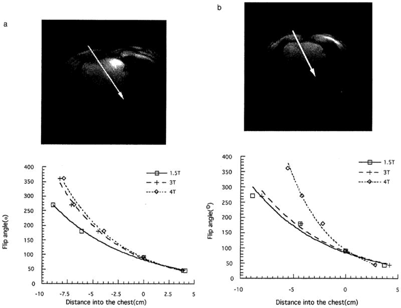
The B₁ profile from the anterior chest wall to the posterior portion of the heart of volunteers 1 (a) and 2 (b). The flip-angle values were taken along the arrows depicted in the transaxial images.

The power needed to generate a 1 ms square pulse of 90° flip at the center of the heart and the corresponding relative ISNR are tabulated in Table 1 for the three field strengths. Also listed is the surface coil efficiency, which was compensated for in the calculation of ISNR. The ISNR increased by nearly a factor of 2.4 from 1.5 to 4 T for both volunteers; correspondingly the power requirements increased by a factor of 9. The field dependence of the ISNR was weaker than the linear relation predicted from previous quasi-static models (20).

DISCUSSION

These data show that, in volunteers of two different body sizes, the ISNR increased with the main field strength up to 4 T. However, the field dependence of the ISNR was weaker than linear, and correspondingly the field dependence of the power deposition was slightly higher than quadratic, as shown in Figs. 6a and 6b. This is consistent with previous body-coil SNR measurements by Hoult et al. (8) and body-coil-loading studies by Röschmann (9). The linear frequency dependence of ISNR at frequencies below 100 MHz is a result of the quasi-static approximation. While this approximation works well below 100 MHz (27, 3), the present results show that the quasi-static approximation overestimates the ISNR in the chest at 3 and 4 T. This result confirms the significance of the conductive and dielectric currents of the body in shaping the RF field distribution. Keltner et al. (14) predicted a superlinear frequency dependence of ISNR in a surface coil–spherical sample model, up to 430 MHz. This was largely due to the enhancing effect of the dielectric resonances in a spherical geometry. This superlinear frequency dependence was not observed in our studies, most likely due to the heterogeneity and irregularity of the chest. Full-wave finite-element simulations with simplified chest models have been able to make predictions consistent with the current experimental results (29).

FIG. 6.

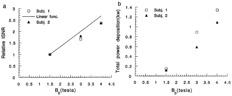
The relative ISNR (a) and total power deposition (b) of both volunteers at 1.5, 3, and 4 T.

The RF field distortion and asymmetry at higher field strengths suggest that the body composition and geometry significantly influence the electrodynamics, as the body serves as a “lens” for the RF field. Under this condition, the phased-array design for signal reception may be difficult in terms of element isolation, and the optimization of element arrangements based on the Biot–Savart law may be invalid. This effect is illustrated by measurements of the mutual isolation of surface coil pairs at 63.5 and 171 MHz. Each surface coil was a 15 cm square separated into four segments by four capacitors placed on the edges of the square, following some commercial designs. Each coil was matched when loaded with volunteer 1. The overlap of the coil pairs was adjusted such that the isolation was maximized in the unloaded condition. At 63.5 MHz, upon loading the Q of each coil decreased from 230 to 25, and the isolation between the pair of coils dropped from 26 to 21 dB. At 171 MHz, the Q of each coil decreased from 129 to 15, and the isolation dropped from 26 to 12 dB. This result is consistent with the increased influence of the body on the RF field distribution. The large loading effect on the coil isolation at 4 T makes the design and use of phased-array receive coils difficult.

The use of phased-array transmit coils to overcome the high power requirement at 4 T also faces the problem of field distortion. In addition to element isolation, it is also difficult to achieve a relatively uniform B₁, from the vector addition of the RF fields of surface coils. The distortion and steep penetration profile of each coil mean that some of the coils must work in subtraction, which negates the efficiency advantage of this approach.

A ninefold increase in power requirements for a 90° pulse in the heart with a surface coil was found between 1.5 and 4 T. This is in reasonable agreement with earlier predictions and underlines the limitations in SAR which are imposed by the 4 T field strength to the design of rapid imaging sequences that take advantage of the increased ISNR.

The ISNR is the upper limit for a specific receive coil configuration and field strength. The apparent SNR of cardiac scans is reduced from the ISNR by many factors such as motion artifacts and spin-relaxation effects. Although the extent of motion artifacts is scan-sequence-dependent, in general it is more pronounced at high field strength (30). In cardiac imaging, the scan repetition time also tends to be short; thus, the driven equilibrium effect reduces the signal level. At high field strength, the longer T₁ values (31) result in larger signal reduction. These issues illustrate the fact that the ISNR is only one aspect of the overall performance evaluation for different field strengths.

In summary, significant improvements in ISNR can be obtained with increasing field strength up to 4 T in the human heart. The increase in ISNR is less than linear with increasing field strength. The increase in ISNR is compromised by increases in power deposition and field distortion which limit the nature of MRI protocols and the use of isolated surface coils in phased arrays at high field. These data are consistent with significant conductive and dielectric effects on the B₁, field and the ISNR in the human chest at these frequencies.

References

- 1.Hoult DI, Lauterbur PC. J Magn Reson. 1979;34:425. [Google Scholar]
- 2.Chen CN, Sank VJ, Cohen SM, Hoult DI. Magn Reson Med. 1986;3:722. doi: 10.1002/mrm.1910030508. [DOI] [PubMed] [Google Scholar]
- 3.Edelstein WA, Glover GH, Hardy CJ, Redington RW. Magn Reson Med. 1986;3:604. doi: 10.1002/mrm.1910030413. [DOI] [PubMed] [Google Scholar]
- 4.Hardy CJ, Bottomley PA, Roemer PB, Redington RW. Magn Reson Med. 1988;8:104. doi: 10.1002/mrm.1910080113. [DOI] [PubMed] [Google Scholar]
- 5.Boska MD, Hubesch B, Meyerhoff DJ, Twieg DB, Karczmar GS, Matson GB, Weiner MW. Magn Reson Med. 1990;13:228. doi: 10.1002/mrm.1910130206. [DOI] [PubMed] [Google Scholar]
- 6.Wust P, Meier T, Seebass M, Fähling H, Petermann K, Felix R. Int J Hypertherm. 1995;11:295. doi: 10.3109/02656739509022464. [DOI] [PubMed] [Google Scholar]
- 7.Schneider CJ, Kuijer JPA, Colussi LC, Schepp CJ, Van Dijk JDP. Med Phys. 1995;22:755. doi: 10.1118/1.597492. [DOI] [PubMed] [Google Scholar]
- 8.Hoult DI, Chen C-N, Sank VJ. Magn Reson Med. 1986;3:730. doi: 10.1002/mrm.1910030509. [DOI] [PubMed] [Google Scholar]
- 9.Röschmann P. Med Phys. 1987;14:922. doi: 10.1118/1.595995. [DOI] [PubMed] [Google Scholar]
- 10.Hanstock CC, Lunt JA, Allen PS. Magn Reson Med. 1988;7:204. doi: 10.1002/mrm.1910070208. [DOI] [PubMed] [Google Scholar]
- 11.Bomsdorf, Helzel T, Kunz D, Röschmann P, Tschendel O, Wieland J. NMR Biomed. 1988;1:151. doi: 10.1002/nbm.1940010308. [DOI] [PubMed] [Google Scholar]
- 12.Barfuss H, Fischer H, Hentschel D, Ladebeck R, Oppelt A, Wittig R, Duerr W, Oppelt R. NMR Biomed. 1990;3:31. doi: 10.1002/nbm.1940030106. [DOI] [PubMed] [Google Scholar]
- 13.Harpen MD. Phys Med Biol. 1988;33:329. doi: 10.1088/0031-9155/33/3/002. [DOI] [PubMed] [Google Scholar]
- 14.Keltner JR, Carlson JW, Roos MS, Wong STS, Wong TL, Budinger TF. Magn Reson Med. 1991;22:467. doi: 10.1002/mrm.1910220254. [DOI] [PubMed] [Google Scholar]
- 15.Bottomley PA, Andrew ER. Phys Med Biol. 1978;23:630. doi: 10.1088/0031-9155/23/4/006. [DOI] [PubMed] [Google Scholar]
- 16.Harpen MD. Med Phys. 1991;18:1052. doi: 10.1118/1.596646. [DOI] [PubMed] [Google Scholar]
- 17.Foo TKF, Hayes CE, Kang Y-W. Magn Reson Med. 1991;21:165. doi: 10.1002/mrm.1910210202. [DOI] [PubMed] [Google Scholar]
- 18.Martin JT, Smith MB. Abstracts of the Society of Magnetic Resonance in Medicine. Annual Meeting; 1990. p. 512. [Google Scholar]
- 19.Vaughan JT, Harrison J, Chapman BLW, Pan JW, Hetherington HP, Vermeulen J, Evanochko WT, Pohost GM. Abstracts of the Society of Magnetic Resonance in Medicine. Annual Meeting; 1991. p. 1114. [Google Scholar]
- 20.Petropoulos LS, Haacke EM, Brown RW, Boerner E. Magn Reson Med. 1993;30:366. doi: 10.1002/mrm.1910300315. [DOI] [PubMed] [Google Scholar]
- 21.Murphy-Boesch J, Carvajal L, Srinivasan R. Abstracts of the Society of Magnetic Resonance in Medicine. Annual Meeting; 1990. [Google Scholar]
- 22.Hoult DI, Richards RE. J Magn Reson. 1976;24:71. doi: 10.1016/j.jmr.2011.09.018. [DOI] [PubMed] [Google Scholar]
- 23.Wen H, Chesnick AS, Balaban RS. Magn Reson Med. 1994;32:492. doi: 10.1002/mrm.1910320411. [DOI] [PMC free article] [PubMed] [Google Scholar]
- 24.Stollberger R, Wach P, Mckinnon G, Justich E, Ebner F. Abstracts of the Society of Magnetic Resonance in Medicine. Annual Meeting; 1988. [Google Scholar]
- 25.Ṡimunić D, Wach P, Renhart W, Stollberger R. IEEE Trans Biomed Eng. 1996;43:88. doi: 10.1109/10.477704. [DOI] [PubMed] [Google Scholar]
- 26.Mansfield P, Morris PG. NMR Imaging in Biomedicine. Suppl 2. Vol. 312. Academic Press; New York: 1982. Advances in Magnetic Resonance. [Google Scholar]
- 27.Bottomley PA, Edelstein WA. Med Phys. 1981;8:510. doi: 10.1118/1.595000. [DOI] [PubMed] [Google Scholar]
- 28.Glover GH, Hayes CE, Pelc NJ, Edelstein WA, Mueller OM, Hart HR, Hardy CJ, O’Donnell M, Barber WD. J Magn Reson. 1985;64:255. [Google Scholar]
- 29.Singerman RW, Denison TJ, Wen H, Balaban RS. J Magn Reson. 1997;125:72. doi: 10.1006/jmre.1996.1073. [DOI] [PubMed] [Google Scholar]
- 30.Wood ML, Henkelman RM. Magn Reson Imaging. 1986;4:387. doi: 10.1016/0730-725x(86)91067-2. [DOI] [PubMed] [Google Scholar]
- 31.Duewell SH, Ceckler TL, Ong K, Wen H, Jaffer F, Chesnick SA, Balaban RS. Radiology. 1995;196:551. doi: 10.1148/radiology.196.2.7617876. [DOI] [PubMed] [Google Scholar]