Latent Regression Analysis

Abstract

Finite mixture models have come to play a very prominent role in modelling data. The finite mixture model is predicated on the assumption that distinct latent groups exist in the population. The finite mixture model therefore is based on a categorical latent variable that distinguishes the different groups. Often in practice distinct sub-populations do not actually exist. For example, disease severity (e.g. depression) may vary continuously and therefore, a distinction of diseased and not-diseased may not be based on the existence of distinct sub-populations. Thus, what is needed is a generalization of the finite mixture’s discrete latent predictor to a continuous latent predictor. We cast the finite mixture model as a regression model with a latent Bernoulli predictor. A latent regression model is proposed by replacing the discrete Bernoulli predictor by a continuous latent predictor with a beta distribution. Motivation for the latent regression model arises from applications where distinct latent classes do not exist, but instead individuals vary according to a continuous latent variable. The shapes of the beta density are very flexible and can approximate the discrete Bernoulli distribution. Examples and a simulation are provided to illustrate the latent regression model. In particular, the latent regression model is used to model placebo effect among drug treated subjects in a depression study.

1 Introduction

Consider the distribution of a continuous variable measured on a population. If the population is homogeneous, the distribution of the variable may be symmetric and unimodal. If the population changes, say due to an evolutionary force, the distribution may become skewed in the direction of the change. Eventually, the population may evolve into two distinct sub-populations, and the distribution of the variable would become a 2-component finite mixture. Similarly, in a clinical trial, the severity of symptoms for patients at baseline may be expected to be homogeneous, symmetric and unimodal. As the trial progresses, the distribution of symptom severity may become skewed in the direction of improvement. If the population consists of two sub-populations (e.g. those who’s symptoms remit and those who’s symptoms do not remit), a 2-component finite mixture model would result.

Motivation for this paper is the investigation of placebo effect (latent predictor) on symptoms improvement (continuous outcome) in psychiatric clinical trials. The goal is to develop a flexible model that can characterize the latent placebo effect, which can be discrete (presence vs. absence) or continuous (degree of placebo effect). The questions of interest are: does the population consist of two latent sub-populations (those who experience placebo effect and those who do not)? Or does the placebo effect vary continuously, possibly having a skewed distribution? Does the placebo effect evolve over the course of the clinical trial, say, starting with an initial skewing effect that eventually leads to the formation of latent subgroups?

The problem of modelling and estimating parameters in populations with distinct latent subgroups is a classical statistical problem that remains an active area of methodological development. A common nonparametric approach to this problem for continuous data is cluster analysis using algorithms such as the well-known k-means algorithm (e.g. Hartigan and Wong, 1979; MacQueen, 1967). Finite mixture models (e.g. Day, 1969; Fraley and Raftery, 2002; Titterington et al., 1985) are model-based approaches to that problem. For instance, normal distributions are often assumed for the components of the mixture and maximum likelihood is used to estimate the parameters of the different latent sub-populations. Finite mixture models have been extended to mixtures of different objects, such as generalized linear regressions (e.g. Wedel and DeSarbo, 1995), or random effects models for longitudinal data, i.e. the growth mixture models (Muthén and Shedden, 1999; Muthén, 2004; James and Sugar, 2003). The analogue of the finite mixture model for categorical outcomes are latent class models (e.g. Goodman, 1974). If a set of predictors are available, then the latent class model for categorical outcomes can be extended to latent class regression models (e.g. Bandeen-Roche et al., 1997; Leisch, 2004; Wedel and DeSarbo, 1995). A further generalization for latent class regression is to model the response on latent factors (Guo et al., 2006), as in a factor analysis.

All of these models attempt to identify distinct latent groups in the population. Often, a very fundamental question needs to be addressed first: do distinct sub-populations even exist? If distinct sub-populations do not exist, it might not be clear what is the utility of fitting mixtures or latent class models. The latent regression model proposed in this paper provides a flexible framework for answering the question on the nature of the underlying latent variable (continuous or discrete) in a population.

In the placebo effect example, let y denote a measured outcome (symptoms severity) and let x denote the latent predictor (placebo effect). Then we could model the outcome y as a simple linear regression on x: y = β₀ + β₁x + ϵ. The problem is that x is unobserved or latent. A regression model with latent (unobserved) predictor is latent regression. If there exist two distinct classes of patients (those who experience a placebo effect and those who do not) then x can be expressed as a 0–1 binary indicator regressor and the latent regression becomes the well-known finite mixture model (see Section 2). On the other hand, if the placebo effect can not be characterized as present or absent, but rather its strength varies continuously among patients from completely absent to present and very strong, then the latent x must be continuous and a latent regression model with continuous predictor is the result. To study the efficacy of drug treatments, the nature of the placebo effect needs to be understood. Knowing whether or not a distinct class of placebo responders exists could inform treatment protocols. The latent regression model proposed in this paper allows a flexible shape distribution to the underlying latent mechanisms in the placebo effect problem.

The latent regression model is defined in Section 2 and maximum likelihood estimation of the parameters is described in Section 3. A simulation experiment is reported in Section 4 to illustrate the latent regression model and contrast it with the finite mixture model. Examples are provided in Section 5 including the placebo effect example that motivated this development. Finally, the paper is concluded in Section 6. Throughout the paper, boldface notation is used to denote matrices and vectors.

2 Latent Regression Model

Consider a simple linear multivariate regression model

$$\mathit{y}={\beta }_0+{\beta }_{1}x+\mathit{ϵ},$$ (1)

where y is a p-variate response vector, β₀ and β₁ represent p-variate intercept and slope vectors and ϵ is a mean zero error independent of the predictor x with covariance matrix Ψ. When the predictor x is unobserved or latent in (1), we shall call the model a latent regression model and our goal is to estimate the parameters of the model when x is unobserved.

Moustaki and Knott (2000) consider a latent regression model in the framework of generalized latent trait models, where a univariate outcome y is regressed on a standard normal latent predictor. It is stipulated that the marginal distribution of the outcome is also normal. However, if the latent regressor x is standard normal and the error ϵ in the regression model is normal with variance σ², then the marginal distribution of the observed outcome is N(β₀;β² ₁ + σ²), in which case the slope β₁ is confounded with the error variance and the model will not be identifiable.

If the population consists of two distinct but latent sub-populations, then the predictor x in (1) has a Bernoulli distribution. Let p = P(x = 1) and assume ϵ has a N(0,Ψ) distribution, where Ψ is a positive-definite covariance matrix. Then the marginal density f(y) of y is the well-known finite mixture model:

$$\begin{array}{ccc}f(\mathit{y})\hfill & =\hfill & {\displaystyle \sum _{x}f(x,\mathit{y})}\hfill \\ \hfill & =\hfill & P(x=0)f(\mathit{y}|x=0)+P(x=1)f(\mathit{y}|x=1)\hfill \\ \hfill & =\hfill & (1-p)N(\mathit{y};{\mathit{\mu }}_1,\mathbf{\Psi })+pN(\mathit{y};{\mathit{\mu }}_2,\mathbf{\Psi })\hfill \end{array}$$ (2)

where μ₁ = β₀, μ₂ = β₀ + β₁, and N(y;μ,Ψ) denotes a multivariate normal density function with mean vector μ and covariance matrix Ψ.

The Bernoulli distribution has all its probability mass at 0 and 1. A natural way to generalize the finite mixture model is to replace the 0–1 Bernoulli predictor by a continuous distribution on the interval (0, 1) that admits “U”-shaped densities. A natural choice for the distribution of x is the beta distribution with density g(x; a, b) defined in terms of parameters a and b:

$$g(x;a,b)=\frac{\mathrm{\Gamma }(a+b)}{\mathrm{\Gamma }(a)\mathrm{\Gamma }(b)}{x}^{a-1}{(1-x)}^{b-1},0<x<1.$$ (3)

The family of beta distributions produces a wide variety of density shapes including “U”-shaped densities which provide a continuous generalization of the discrete Bernoulli distribution. Note that for a given Bernoulli probability p, the beta distribution with parameters a and b = a(1 − p)/p has mean p and variance ab=[(a + b + 1)(a+b)²]. As a goes to zero, b will also go to zero, the mean of the beta distribution remains equal to p, while the variance converges to the Bernoulli variance p(1 − p) and the beta distribution degenerates into a Bernoulli distribution with success probability p.

We shall assume the error ϵ in (1) is independent of x and initially we will also assume that it has a normal distribution N(0;Ψ). In Section 5 we will consider a skew-normal distribution (e.g. Azzalini and Capitanio, 1999) for ϵ to provide greater exibility of the model. The outcome y in (1) is therefore a convolution of a beta random variable with a normal random variable. The joint density for x and y in (1) is

$$f(x,\mathit{y})=f(\mathit{y}|x;{\beta }_0,{\beta }_1,\mathbf{\Psi })g(x;a,b)=N(\mathit{y};{\beta }_0+{\beta }_{1}x,\mathbf{\Psi })g(x;a,b)$$ (4)

where g(x; a, b) is the beta distribution given in (3). The marginal density of the outcome is

$$f(\mathit{y})={\displaystyle {\int }_0^1\frac{1}{\sqrt{2\pi }}}{\mathbf{\Psi }}^{-1/2}\text{exp}\{-{(\mathit{y}-{\beta }_0-{\beta }_{1}x)}^{\prime }{\mathbf{\Psi }}^{-1}(\mathit{y}-{\beta }_0-{\beta }_{1}x)/2\}g(x;a,b)dx,$$ (5)

which is an example of an infinite mixture where the mixing density is a beta.

Another well-known example of a continuous mixture using a beta mixing distribution is the beta-binomial distribution for discrete count outcomes. For example, Dorazio and Royle (2003) consider an infinite mixture using a beta mixing distribution in the capture-recapture problem of estimating population size where the probability of capture can vary continuously. They also argue, as do we, that even though finite mixtures are often used to accommodate model heterogeneity, an infinite mixture is often a more appropriate model (Dorazio and Royle, 2003, page 352).

Identifiability of the latent regression model follows from Bruni and Koch (1985) under certain regularity conditions (see the Appendix) with the following exceptions: (i) in degenerate cases, β₁ = 0 or when the latent beta distribution concentrates all its probability mass either at zero or one, (ii) if x is the latent beta(a, b), then 1 − x is beta(b, a) and β₀ + β₁x + ϵ = (β₀+β₁)−β₁(1 − x)+ ϵ are two representations of the same model. There are parameter configurations for the latent regression model that are nearly unidentifiable. For example, in the univariate case, the latent regression model obtained by convolving a uniform (0, 1) with a standard normal distribution produces a density given by f(y) = Φ(y)−Φ(y −1), where Φ is the standard normal cumulative distribution function. This density is almost indistinguishable from a normal density with mean μ = 1/2 and variance σ² = 13/12, which can be expressed as a degenerate latent regression model with β₀ = 1/2, β₁ = 0 and error variance 13/12. The next sections describe maximum likelihood estimation of the parameters in the latent regression model. If the algorithms described below have difficulty converging, then one possible explanation could be the near un-identifiability of the latent regression model for certain parameter configurations.

3 Estimation

This section describes an EM algorithm applied to the joint likelihood of the response and the latent predictor. Additionally, a quasi-Newton method is also described for finding the maximum likelihood estimates for the marginal log-likelihood of the response y only.

3.1 An EM-Algorithm

Given the complete data (x₁, y₁), …, (x_n, y_n) in (1), it follows from (4) that the log-likelihood is

$$\begin{array}{ccc}l({\beta }_0,{\beta }_1,\mathbf{\Psi },a,b)\hfill & =\hfill & -\frac{n}{2}\text{log}(2\pi )-\frac{n}{2}\text{log}\left|\mathbf{\Psi }\right|\hfill \\ \hfill & \hfill & -{\displaystyle \sum _{i=1}^n{({\mathit{y}}_i-{\beta }_0-{\beta }_1{x}_i)}^{\prime }{\mathbf{\Psi }}^{-1}({\mathit{y}}_i-{\beta }_0-{\beta }_1{x}_i)/2+{\displaystyle \sum _{i=1}^n\text{log}(g(x_i;a,b)).}}\hfill \\ \hfill & \hfill & \hfill \end{array}$$

Because x is latent, the EM algorithm (Dempster et al., 1977) proceeds by maximizing the conditional expectation of the log-likelihood given the vector of observed outcomes y:

$$E[l({\beta }_0,{\beta }_1,\mathbf{\Psi },a,b)|\mathit{y}].$$

At each iteration of the EM algorithm, this conditional expectation is computed using the current parameter estimates. For the normal finite mixture model, closed form expressions exist for the EM algorithm (e.g. McLachlan and Krishnan, 1997, page 68). However, for the latent regression model with a beta predictor, the E-step of the EM algorithm requires numerical integration. In particular, the conditional expectations of x, x², ln(x), and ln(1−x) given the response vector need to be computed. The EM algorithm and the numerical integrations in the simulations and examples that follow were performed using the R-software (R Development Core Team, 2003).

To maximize the expected log-likelihood, we arrange the n response vectors into an n×p matrix Y. In the case of a single latent predictor, we can define a coefficient matrix

$$\beta =\left(\begin{array}{c}{\beta }_0^{\prime }\\ {\beta }_1^{\prime }\end{array}\right)$$

of dimension 2 × p where each of the p columns of β provide the intercept and slope regression coefficients for each of the p response variables. Let X denote the design matrix whose first column consists of ones for the intercept and the second column consists of the latent predictors x_i, i = 1, …, n. The multivariate regression model can be written

$$\mathit{Y}=\mathit{X}\beta +\mathit{ϵ}.$$

The likelihood for the multivariate normal regression model (e.g. Johnson and Wichern, 2005, Chapter 7) can be expressed as

$$L(\beta ,\mathbf{\Psi })={(2\pi )}^{-np/2}\left|\mathbf{\Psi }{|}^{-n/2}\text{exp}\right\{-tr[{\mathbf{\Psi }}^{-1}{(\mathit{Y}-\mathit{X}\beta )}^{\prime }(\mathit{Y}-\mathit{X}\beta )]/2\}.$$ (6)

To apply the EM algorithm, we need to maximize the expectation of the logarithm of (6) conditional on Y with respect to β and Ψ. Let X̃ = E[X|Y] and $(\stackrel{\sim }{\mathit{X}\prime \mathit{X}})=E[\mathit{X\prime }\mathit{X}|\mathit{Y}]$. Note that computing the conditional expectations X̃ and $(\stackrel{\sim }{\mathit{X}\prime \mathit{X}})$ require integrating over the latent predictor x. The conditional expectation of tr[Ψ⁻¹(Y−Xβ)′(Y−Xβ)] with respect to Y is

$$tr[{\mathbf{\Psi }}^{-1}\{\mathit{Y}\prime \mathit{Y}-\mathit{Y}\prime \stackrel{\sim }{\mathit{X}}\beta -\beta \prime \stackrel{\sim }{\mathit{X}}\prime \mathit{Y}+\beta \prime (\stackrel{\sim }{\mathit{X}\prime \mathit{X}})\beta \}].$$ (7)

Let

$$\hat{\beta }={(\stackrel{\sim }{\mathit{X}\prime \mathit{X}})}^{-1}\stackrel{\sim }{\mathit{X}}\prime \mathit{Y}.$$ (8)

Equation (7) can then be re-expressed as

$$tr[{\mathbf{\Psi }}^{-1}\{(\mathit{Y}\prime \mathit{Y}-\widehat{\beta }\prime (\stackrel{\sim }{\mathit{X}\prime \mathit{X}})\widehat{\beta })-(\widehat{\beta }-\beta )\prime (\stackrel{\sim }{\mathit{X}\prime \mathit{X}})(\widehat{\beta }-\beta )\}].$$ (9)

The portion of the trace in (9) involving the parameters β can be written

$$\begin{array}{ccc}tr[{\mathbf{\Psi }}^{-1}(\widehat{\beta }-\beta )\prime (\stackrel{\sim }{\mathit{X}\prime \mathit{X}})(\widehat{\beta }-\beta )]\hfill & =\hfill & tr[(\stackrel{\sim }{\mathit{X}\prime \mathit{X}})(\widehat{\beta }-\beta ){\mathbf{\Psi }}^{-1}(\widehat{\beta }-\beta )\prime ]\hfill \\ \hfill & =\hfill & tr{[(\stackrel{\sim }{\mathit{X}\prime \mathit{X}})}^{1/2}(\widehat{\beta }-\beta ){\mathbf{\Psi }}^{-1}(\widehat{\beta }-\beta )\prime {(\stackrel{\sim }{\mathit{X}\prime \mathit{X}})}^{1/2}].\hfill \end{array}$$

Because $(\stackrel{\sim }{\mathit{X}\prime \mathit{X}})$ and Ψ are positive definite, this last expression is minimized for $\beta =\widehat{\beta }$. Additionally, from standard results for multivariate normal likelihood estimation, the expected log-likelihood will be maximized with respect to Ψ by setting

$$\widehat{\mathbf{\Psi }}=\mathit{Y}\prime \mathit{Y}-\widehat{\beta }\prime (\stackrel{\sim }{\mathit{X}\prime \mathit{X}})\widehat{\beta }.$$ (10)

Thus, the expected log-likelihood is maximized by β̂ and Ψ̂ in (8) and (10). Note that substituting X̃ for X in the usual maximum likelihood formula for the covariance matrix $(\mathit{Y}-\mathit{X}\widehat{\beta })\prime (\mathit{Y}-\mathit{X}\widehat{\beta })/n$ will not produce the correct estimator for Ψ because $(\stackrel{\sim }{\mathit{X}\prime \mathit{X}})\ne \stackrel{\sim }{\mathit{X}}\prime \stackrel{\sim }{\mathit{X}}$.

The Newton-Raphson algorithm was used to maximize log-likelihood for the beta parameters a and b, which requires the imputation of the conditional expectation of ln(x_i) and ln(1 − x_i) given y_i for each observation in place of the unobserved ln(x_i) and ln(1 − x_i). Initial values for the Newton-Raphson algorithm are provided by the method of moments. Initial values for the regression parameters β₀ and β₁ can be obtained from fitting a two-component finite mixture or by a preliminary search over the parameter space. Initial values for Ψ can be obtained using the sample covariance matrix from the raw data.

3.2 Maximizing the Marginal Likelihood

An alternative to applying the EM algorithm to the joint likelihood of (x, y), is to directly maximize the marginal log-likelihood of y based on the marginal density (5). Quasi-Newton algorithms can be applied to the marginal log-likelihood. Because closed form expressions for the marginal density of y, the log-likelihood, its derivatives and the Hessian do not exist, they must be computed numerically (e.g. Thisted, 1991, page 184). In particular, we have implemented the L-BFGS-B method (Byrd et al., 1995) which is available in the R-software (R Development Core Team, 2003) using the “optim” function. This method allows box-constraints on the parameters which guarantees that that parameter estimates stay within the parameter space. In the second example of Section 5.1, a grid search over the parameter space was used to find initial values for the parameters.

3.3 Additional Notes on Estimation

If the true underlying distribution is a two-component mixture, the parameters of the latent beta distribution will go to zero as the EM and quasi-Newton algorithms iterate causing the algorithms to eventually crash when trying to evaluate the integrals. Like the EM algorithm for finite mixtures, the EM algorithm for the latent regression model can sometimes be slow to converge when the likelihood surface is flat. The algorithms are also sensitive to starting values. Numerical integration is required for the latent regression algorithms and this can introduce numerical error in the iterations. The effect of this numerical error can be diminished by evaluating the integrals to a higher degree of numerical precision.

Also, it is well known that singularities occur in the likelihood function for finite mixture models (e.g., see Everitt, 1984). In particular, the likelihood for a finite mixture becomes unbounded by setting a mixture component mean equal to the value of one of the data points and letting the variance for that component go to zero. A similar problem can occur with the latent regression model, if we set β₁ = 0, β₀ = y_i for a given outcome value y_i, and let σ → 0 and the beta regressor parameter a → 0 as well. However, it is easy to show that the marginal density for the outcome is bounded above by $1/\sqrt{2\pi {\sigma }^2}$.

4 A Simulation Experiment

The EM algorithm described in Section 3.1 was tested on simulated univariate data sets (p = 1), using a variety of parameter settings for the latent regression model. For each parameter setting, fifty data sets were simulated, each with a sample size of n = 100. If the latent regressor x has a “U”-shaped distribution, then a histogram of the outcome y will look very similar to a two-component mixture density. Therefore, for each simulated data set, a two-component finite mixture was also fit to the data for the sake of comparison.

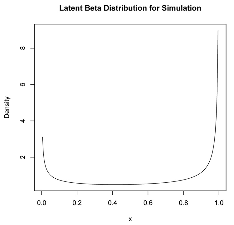
For illustration, this section reports the results from one of the simulations. In this simulation, the latent regressor x had a beta distribution with parameters a = 0.5 and b = 0.3 which produces the “U”-shaped density in Figure 1. The error ϵ had a normal distribution with mean zero and standard deviation σ = 0.5. The regression parameters were set at β₀ = 1 and β₁ = 6. For each simulated data set, the EM algorithm was allowed to iterate 100 times.

Figure 1.

Beta density with a = 0.5 and b = 0.3 for the latent regressor x in the simulation example.

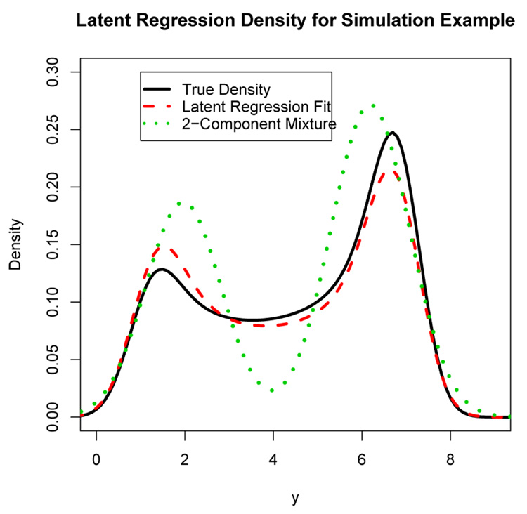
Figure 2 shows the true density for the outcome y (solid curve). One of the purposes of this simulation experiment is to illustrate the fact that bimodal densities do not always results from mixture models. The density in Figure 2 looks like a two-component mixture density with a clear bimodal shape, but it is actually the outcome in a latent regression model with a beta predictor. The dashed curve in Figure 2 is the estimated latent regression density from one of the simulated data sets and the dotted curve represents the estimated two-component finite mixture density from the same data set. The fitted latent regression density curve provides a good fit to the true density, whereas the finite mixture density does a poor job.

Figure 2.

Density of the latent regression outcome y = 1+6x+ ϵ where x has a beta distribution with parameters a = 0.5 and b = 0.3. The error variance is σ² = 0.25. The solid curve is the true density. The dashed and dotted curves are the estimated densities from one of the simulated data sets for the latent regression model and a two-component mixture model respectively.

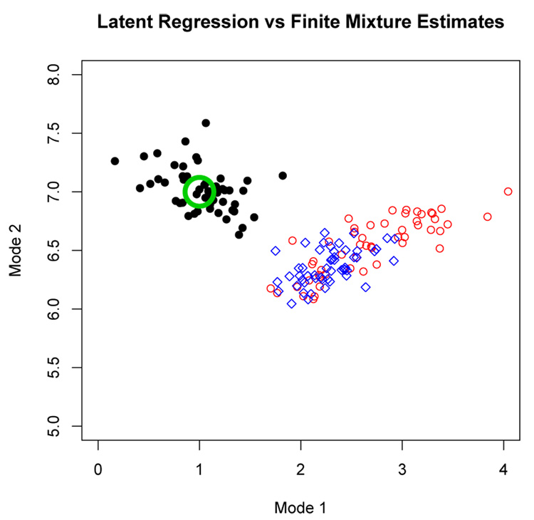
Figure 3 shows the fitted regression parameters for the 50 data sets simulated under a = 0.5 and b = 0.3, after converting μ₁ = β₀ and μ₂ = β₀ + β₁ so that the latent regression results can be compared to fitting a finite mixture model (2); under the finite mixture model μ₁ and μ₂, which represent the conditional mean of y given x = 0 and x = 1, are also the two modes of the distribution of y. The large open circle shows the true values of μ₁ and μ₂. The small solid dots represent the latent regression model estimates of μ₁ and μ₂. The small open circles represent the estimated mixture component means from fitting a two-component finite normal mixture (with unequal component variances). For comparison sake, estimates of the cluster means from the k-means clustering algorithm are also shown (small diamonds). From Figure 3 it is clear that although the density of the outcome resembles a mixture density, the fitted parameters from a finite normal mixture model completely miss the two modes of the underlying distribution, whereas the estimates from the correct latent regression model appear unbiased in this example. It is also interesting to note that the finite mixture estimates are more spread out than the k-means cluster means estimates.

Figure 3.

The large open circle marks the true value of (μ₁; μ₂) = (1, 7). The solid circles represent the estimates from the latent regression model. The small open circles represent the estimates from fitting a standard two-component mixture model. The tiny diamonds represent estimates from running the k-means clustering algorithm.

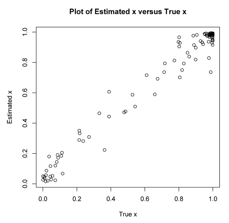
Figure 4 shows a scatterplot of E[x|y_i] versus the true value of x_i from one of the simulations where the conditional expectation was computed using the parameter estimates found at the 100th iteration of the EM algorithm. The correlation between the x_i and E[x|y_i] in Figure 4 is 0.985.

Figure 4.

Scatterplot of E[x|y_i] versus x_i for one of the simulated data sets using parameter estimates from 100 iterations of the EM algorithm. The correlation between the x_i and E[x|y_i] is 0.985.

Simulations with other latent regression parameter settings gave similar results to those reported here. The simulation example presented here illustrates that fitting a finite mixture model to latent regression data will not only give the wrong results but will also give the mistaken impression that the population consists of two well-defined sub-populations. On the other hand, if the underlying distribution is indeed a mixture, then the latent beta parameters a and b will go to zero.

5 Examples

This section illustrates the latent regression model with two univariate and one multivariate example. The first example, the modelling of placebo effect, provided the motivation for developing the latent regression model.

5.1 Evolution of a Placebo Effect

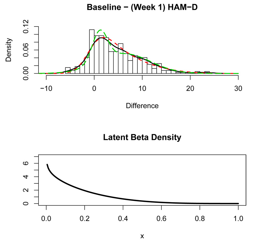
Substantial placebo effect has been observed in the treatment of many psychiatric illnesses such as depression. A subject treated with an active drug may improve in part due to a placebo effect (e.g. Walsh et al., 2002; Khan and Brown, 2001; Brown et al., 1992; Thase, 1999; Mulrow et al., 1999) which is a latent characteristic. The top panel of Figure 5 shows a histogram for n = 393 subjects, all of them ultimately rated as treatment responders in an open label study of depression where all subjects received Prozac for 12 weeks (McGrath et al., 2000). The histogram shows the change in the depression symptoms severity between baseline (week 0) and week 1, measured on the Hamilton Depression Rating scale (HAM-D), where a positive change indicates decreased depression from baseline to week 1. The top panel of Figure 5 shows a skew-right distribution of mostly positive changes indicating varying degrees of improvement among most subjects. However, it is believed that the pharmacological properties of this drug are such that the onset of action is usually several weeks after initiation of treatment. If this is true, then the mood improvements after 1 week shown in Figure 5 must be primarily due to other factors such as a placebo effect. In fact, because the placebo effect is known to exist in depression studies and that the placebo effect tends to improve mood, it seems reasonable to attribute the latent regressor to a placebo effect in this example.

Figure 5.

Top panel: Histogram of the change (Baseline - Week 1) in severity of depression measured by HAM-D scores for subjects treated with Prozac. Overlaid is a nonparametric density estimate (solid curve), the latent regression density estimate (short-dashed curve), and a two-component finite mixture density estimate (long-dashed curve). Bottom Panel: Estimated beta density for the latent regressor.

Because the placebo effect is latent, we model the change in severity from baseline to week 1, y, as a function of the strength of the subject’s placebo effect x using latent regression. If x in (1) is Bernoulli, the model postulates that there exist two types of subjects: those who experience a placebo effect and those who do not. If x is continuous, the model states that each subject experiences a placebo effect of varying degree. The solid curve shown in the top panel of Figure 5 is a nonparametric density estimate of y; the density estimate from the latent regression model with beta latent regressor is shown as a short-dashed curve. The long-dashed curve is a density estimate from fitting a two component finite mixture model. The beta parameter estimates from the latent regression were found to be â= 0.897 and b̂= 4.313. The estimated latent regression model is ŷ = −0.629 + 30.849x and the error standard deviation was estimated to be σ̂ = 2.278. The fit of the latent regression density in Figure 5 coincides with the nonparametric density quite well, whereas the finite mixture density does not coincide as well with the nonparametric density estimate.

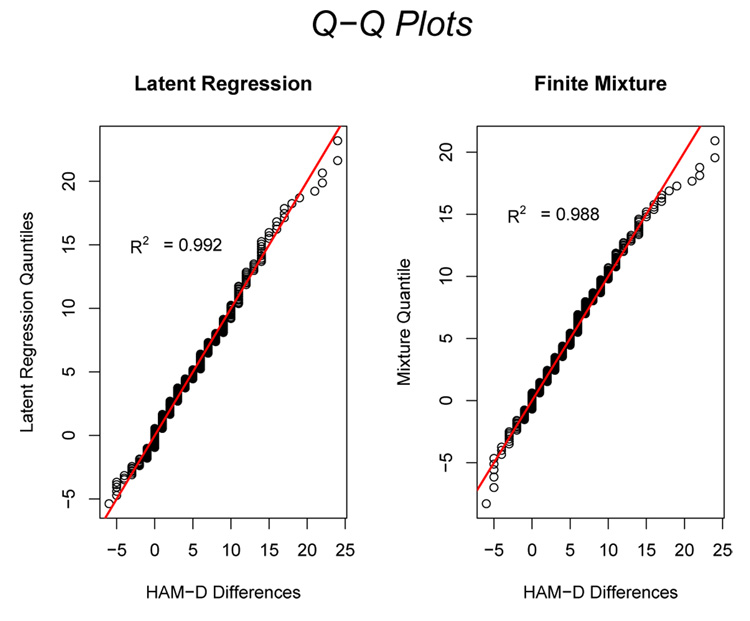
In order to determine which model (latent regression or the finite mixture) provides a better fit to the data, we borrow the idea underlying the Shapiro-Wilks test for normality (Shapiro and Wilks, 1965). We compute the squared correlation R² between the quantiles of the observed data and the corresponding quantiles of the respective model of interest: latent regression or finite mixture. Figure 6 shows the quantile-quantile or Q-Q plot for the latent regression (left panel) and the 2-component finite mixture (right panel) distributions. The 45⁰ diagonal line is plotted for reference. The R² for the latent regression and finite mixture models are 0.992 and 0.988 respectively indicating that both models fit the data well, with the latent regression providing a slightly better fit. Figure 6 shows that both the latent regression and finite mixture models give roughly straight line relations to their respective quantiles except in the right tail where the finite mixture model deviates more strongly than the latent regression model from the data quantiles.

Figure 6.

Q-Q plots for the latent regression model (left panel) and the 2-component finite mixture model (right panel) for the week 1 improvement data. The 45⁰ diagonal line is plotted for reference.

The beta distribution for the latent predictor shown in the bottom panel of Figure 5 supports the contention that there are not two distinct classes of subjects (those who do and do not experience a placebo effect) when treatment begins, but instead the placebo effect varies over a continuum according to a strongly skewed right distribution with the proportion of people experiencing a placebo effect of a given magnitude decreasing as the magnitude of this effect increases. According to the latent regression model, the maximum placebo effect corresponds to a change score of around 30 points decrease on the Hamilton Depression rating scale. However, only a very small proportion of the population experiences such large effect (less than $\frac{1}{100}$ of 1%) and less than 5% had strength of the placebo effect larger than one half of the maximum effect of 30 points.

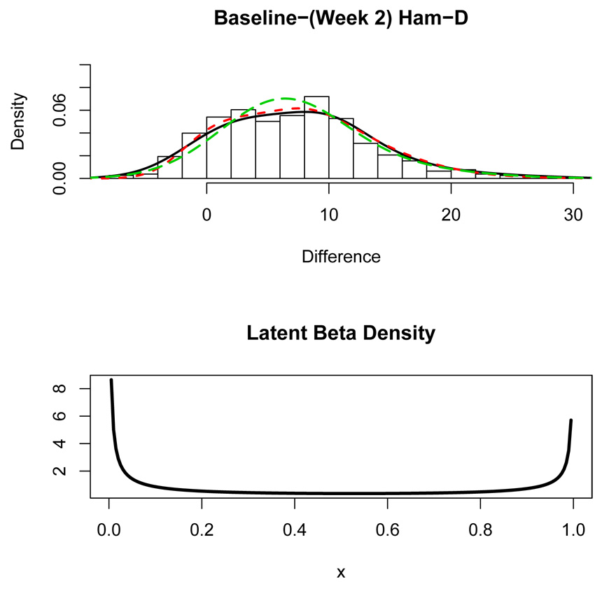
To assess how the latent placebo effect evolves over time, a latent regression model was also fit to the changes: (Baseline) – (Week 2) HAM-D. The fit of the latent regression model with a normal error was somewhat poor in the right tail of the distribution due to skewness in the positive direction shown in Figure 7. To add greater flexibility to the latent regression model, a skew-normal distribution (e.g. Azzalini and Capitanio, 1999; Johnson et al., 1988) was proposed for the error ϵ with density

$$2\varphi (z/\sigma )\mathrm{\Phi }(\alpha z/\sigma )/\sigma ,$$

where α is the skewness parameter and ϕ is the density and Φ is the cumulative distribution function of the standard normal random variable. The degree of skewness increases with α and α > 0 causes the distribution to be skewed to the right. The latent regression model was fit using the L-BFGS-B algorithm (Byrd et al., 1995) described in Section 3.2. The fitted model was found to be ŷ = −2.21 + 9.37x with beta parameters â = 0.213 and b̂ = 0.301. The error standard deviation was estimated to be σ̂ = 7.540 and the skewness parameter was estimated to be α̂ = 3.243. Figure 7 shows a histogram of the change in depression severity from baseline to week 2 along with a nonparametric density curve (solid curve). The estimated density of the outcome from the fitted latent regression model with skew-normal distribution of the error is plotted using the short-dashed curve. As Figure 7 shows, the latent regression model appears to fit the data very well. There is a hint of bimodality in the histogram in Figure 7 and correspondingly, the estimated beta distribution for the latent placebo effect shown in the bottom panel of Figure 7 has a very distinct “U”-shape.

Figure 7.

Top Panel: Histogram of week 2 changes in HAM-D scores from baseline. The solid curve is a nonparametric density estimate and the short-dashed curve is the estimated density from the latent regression. The long-dashed curve is the fitted two-component normal mixture density. Bottom Panel Estimated beta distribution for the latent regressor.

Thus, initially (at week 1) placebo effects vary continuously, ranging from very weak to quite strong resulting in a placebo effect distribution skewed in the direction of improvement, as on Figure 5 bottom panel. At week 2 the placebo effects still vary continuously, but we begin to see a segmentation into two groups where one group has little to no placebo effect and the other group has much stronger and distinct placebo effects. If the experimental drug Prozac does not begin to have an effect until after week 2, as some researchers believed, then it makes sense to attribute most of the observed outcome in Figure 5 and Figure 7 to a placebo effect. However, a skew-normal error was needed in the model for week 2 to account for the right tail skewness evident in the histogram in Figure 7. What does this mean? One might consider the skewness in the errors to be evidence of a beginning chemical effect of the drug. Alternatively, the skewed distribution of the error might reflect the action of a positive placebo effect, while the latent regressor x in the model for the change at week 2 might actually be corresponding to the specific effect of the drug. Incidentally, a two-component finite mixture model with normal components was fit to the data using the EM-algorithm but the algorithm was very slow to converge and produced a unimodal density estimate shown by the long-dashed curve in the top-panel of Figure 7. The Q-Q R² for the latent regression and the finite mixture fits to the week 2 data are 0.9934 and 0.9938 respectively indicating that both models fit the data very well.

5.2 Ultra-Marathon Race

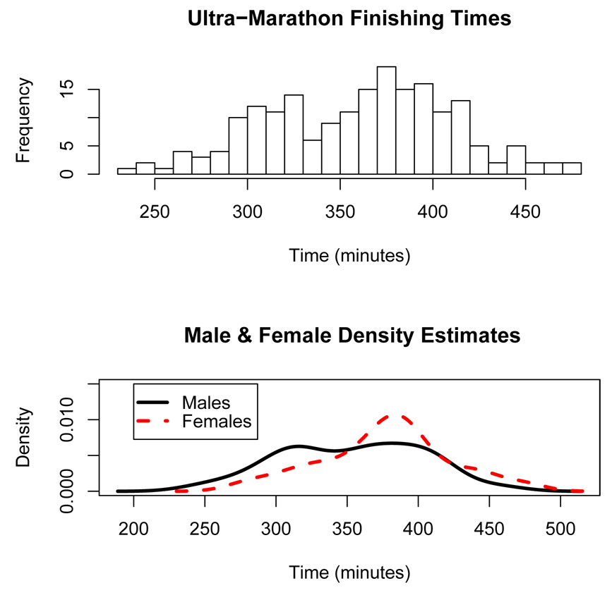
A histogram of the finishing times in the Skyline 50 kilometer Ultra-Marathon run on August 4, 2002 in Castro Valley, California is shown in top panel of Figure 8. The histogram appears bimodal and one can postulate that perhaps the bimodality is due to a mixture of male and female runners. However, the bottom panel of Figure 8 shows separate nonparametric density estimates for males (solid curve) and females (dashed curve) each of which look similar to 2-component finite mixture densities. A natural latent regressor variable x in this example is the degree of training the runners underwent in preparing for the race. If the latent regressor x represents the degree of training, then it may be reasonable to model x as a continuous variable representing the number of hours in training or the number of miles that were run to prepare for the race. On the other hand, a Bernoulli x may correspond to race participants belonging to two separate classes: elite competitive athletes and recreational athletes, for instance.

Figure 8.

Top Panel: Histogram of the finishing times in the Skyline Ultra-Marathon. Bottom Panel: Nonparametric density estimates of the finishing times for males (solid curve) and female (dashed curve) runners.

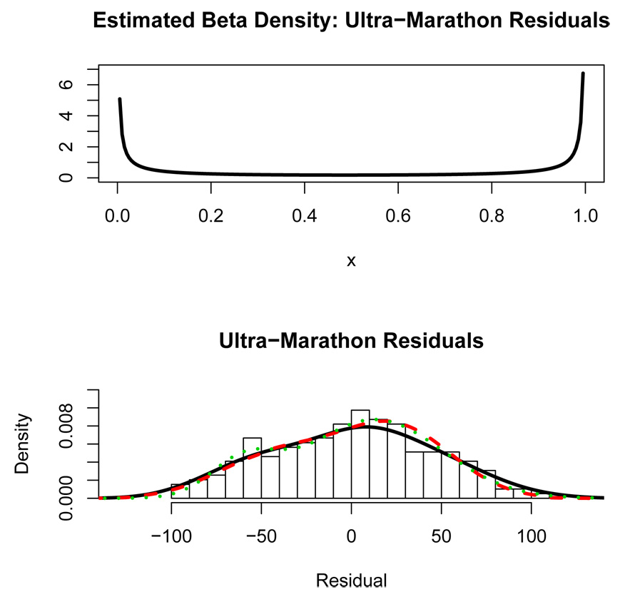
The ultra-marathon data set also has the age of the runners. After controlling for age and sex, the question remains whether there are two distinct classes of runners or if there is a continuous latent variable underlying performance in the ultra-marathon. A latent regression model and a finite mixture model (using the EM algorithm) were fit to the residuals. The EM-algorithm for the latent regression model using a beta distribution for the predictor was very sensitive to starting values in this case. During successive iterations of the EM algorithm, the beta parameters in the latent regression model were approaching zero. Therefore as the algorithm iterated, the beta distribution was converging to a degenerate Bernoulli 0–1 distribution indicating that the underlying distribution is consistent with a two-component mixture. As the beta distribution degenerates into a Bernoulli distribution, eventually the numerical integration required for the EM algorithm will fail. Using the default settings for the “integrate” function in R (R Development Core Team, 2003), the beta parameter values found by the EM algorithm right before the integration failed were a = 0.135 and b = 0.082. The beta density for these parameter values is shown in top panel of Figure 9. The beta density in Figure 9 looks like an approximation to a Bernoulli distribution. These values for a and b should not be construed as maximum likelihood estimates of the beta parameters in the latent regression model. Instead, since the beta parameter values were approaching zero, the implication is that the underlying model is a mixture. Note that the accuracy of the numerical integration could be increased so that the EM algorithm could continue to iterate, but the point here is that the underlying distribution appears to be the degenerate case of the latent regression model, i.e. a two-component mixture. Density estimates from the latent regression fit (at the point the EM algorithm stopped) and the fitted finite mixture model are also shown overlaying the residual histogram in the bottom panel of Figure 9 (dashed and dotted curves respectively). As can be seen, the latent regression density curve closely resembles the finite mixture density curve which visually appears to be a good fit to the residual distribution. In this example, the latent regression modelling of the data indicates the existence of two well-defined mixture components. We hypothesize that these two groups correspond to elite/serious runners and recreational runners.

Figure 9.

Top panel: Latent beta density for the ultra-marathon residuals at the point the algorithm stopped. Bottom panel: Histogram of ultra-marathon residuals from fitting the finishing time on age and sex. The solid curve is a nonparametric density estimate. The dashed curve is the latent regression fit to the residuals and the dotted curve is the 2-component normal mixture fit.

5.3 South African Heart Disease

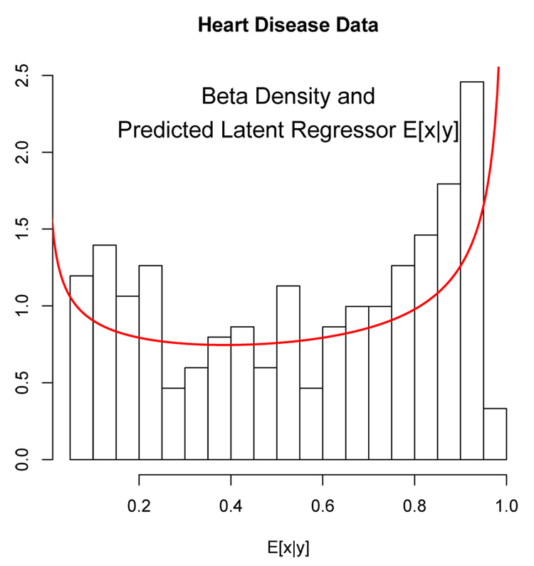
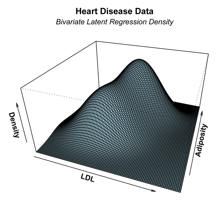
In this subsection we present a bivariate example of the latent regression model. The data is a subset of the Coronary Risk-Factor Study (Rousseauw et al., 1983) and is discussed in (Hastie et al., 2001, Page 100). The goal of this study was to examine risk factors associated with ischemic heart disease. The data was collected on white males between 15 and 64 years of age. We shall fit a latent regression model on the subset of those men who have not experienced myocardial infarction (MI) and we shall illustrate the latent regression model using variables: (1) low density lipoprotein cholesterol (LDL) and (2) adiposity. The EM algorithm, described in Section 3.1 was used to fit a bivariate latent regression model to the data. Figure 10 shows a histogram of the expected latent predictor x̂_i = Ê[x|y_i] where the conditional expectation is computed using the estimated model parameters. Overlayed with the histogram is the estimated latent beta density with beta parameters â = 0.74 and b̂ = 0.59. Figure 11 shows the corresponding estimated bivariate density function of the LDL and adiposity responses. A bimodal shape is evident in the three-dimensional plot due to the “U”-shaped latent density.

Figure 10.

Histogram of the expected latent beta predictors computed from x̂_i = Ê[x|y_i]. Overlaid is the estimated latent beta density.

Figure 11.

The estimated bivariate latent regression density for the the LDL and adiposity distribution

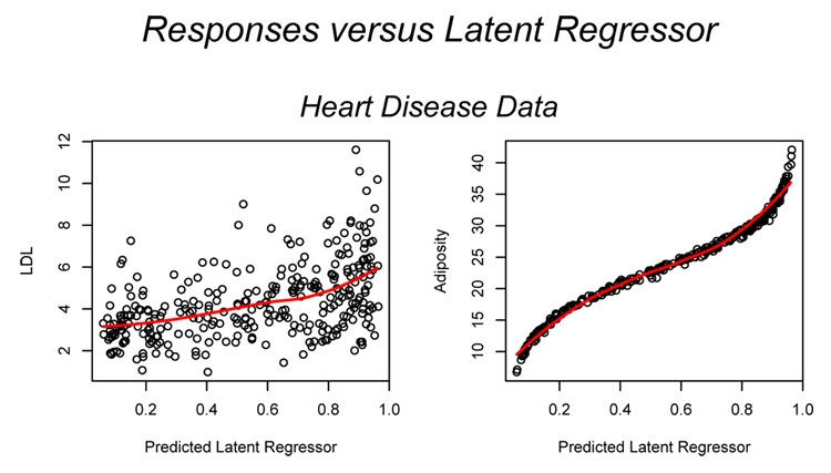
Figure 12 shows plots of LDL (left panel) and adiposity (right panel) versus the predicted latent regressor x̂_i = Ê[x|y_i]. A nonparametric loess curve is also plotted in each panel to provide an indication of the relation between the responses and the latent predictor. Both responses increase with increases values of the latent predictor. However, adiposity is much more strongly (and non-linearly) related to the latent regressor than LDL. The likely explanation for this is that adiposity accounts for most of the variability in the data: the variance of adiposity is 60.6 compared to 3.1 for LDL.

Figure 12.

Plots of LDL (left panel) and Adiposity (right panel) versus the predicted latent regressor x̂_i = Ê[x|y_i]. A nonparametric loess curve is also plotted in each panel.

The proportion of variability in the bivariate response explained by latent regressor can be computed as

$$R^2=1-\frac{\text{trace}(\widehat{\mathbf{\Psi }})}{\text{trace}({\mathit{S}}_{\mathit{y}})},$$

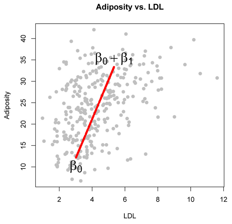
where Ψ̂ is the estimated error covariance matrix from (1) and S_y is the sample covariance matrix of the raw data. In this example, R² = 0.758 indicating that about 76% of the variability in LDL and adiposity can be explained by the latent predictor. Note that because the latent regressor is univariate, the variability in the multivariate response explained by the latent regression relation, β₀ + β₁x from (1), is along a single dimension. Figure 13 shows a bivariate scatterplot of adiposity versus LDL. Overlaid is the line β̂₀ + β̂₁x for values of x from 0 to 1. Interestingly, the line in Figure 13 corresponds almost exactly with the first principal component axis of the response.

Figure 13.

Heart Disease Data: Adiposity versus LDL. The line represents the one-dimensional direction of variability explained by the latent regressor x.

A two-component finite mixture model stipulates that there are two distinct classes of subjects in terms of LDL and adiposity. Therefore, according to the finite mixture model, the response for an individual is equal to the mean of the mixture component the individual belongs plus a random error. A reasonable alternative is that LDL and adiposity each vary continuously where distinct groups do not exist. The predicted latent variable, x̂_i = Ê[x|y_i], can then be used to assign a level of risk for MI with higher values corresponding to higher risk level. The “U”-shaped latent predictor in Figure 10 indicates that men tend to be segregating at the low and high ends of the risk distribution with a greater proportion of men at the higher end of the risk distribution than at the lower end.

For multidimensional data, the finite mixture model is defined by more parameters than the latent regression model. For instance, in two dimensions, the 2-component mixture has 11 free parameters while the latent regression model has only 9 parameters. The difference in the number of parameters for the mixture and latent regression models grows larger as the dimension increases. The additional flexibility enjoyed by the mixture model is in terms of the covariance structure which can differ between the mixture components. The multidimensional latent regression model is better suited for data following an allometric extension model (Bartoletti et al., 1999; Tarpey and Ivey, 2006) where the populations differ (either continuously or between discrete groups) along a common first principal component axis.

6 Discussion

We have introduced a simple linear regression model with a beta-distributed latent predictor that generalizes the two-component finite mixture model. The finite mixture model may be inappropriate when the claim of distinct latent groups in the population is made to explain heterogeneity that is actually due an underlying continuous latent variable. The latent regression model can be used assess the evidence for finite mixture.

There are several generalizations to consider for the latent regression model. For instance, another possible distribution to consider for the latent predictor is a logistic normal (Aitchison and Shen, 1980): x = e^a+bz/(1 + e^a+bz), where z ~ N(0, 1). The density for this x produces a wide variety of shapes including “U”-shapes. Fitting the latent regression model with a logisticized normal produced similar results as those obtained using a beta distribution in the examples considered here. For the placebo effect example in Section 5.1, a skew-normal distribution was used to model the error in the latent regression model for the week 2 improvement in depression. An alternative with even greater exibility is to model the error as a finite mixture of normals (Bartolucci and Scaccia, 2005).

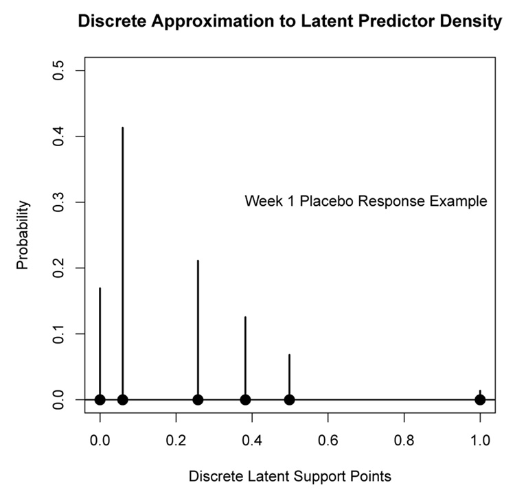
An alternative to directly estimating the parameters of the underlying latent density (e.g. beta distribution) is to estimate a discrete approximation to the latent density via a finite mixture. In particular, in the univariate case (p = 1) let μ̂₁, …, μ̂_k, denote the k ordered finite mixture component means with corresponding prior probabilities π̂₁, …, π̂_k, estimated by fitting a k-component finite mixture. Let β̂₀ = μ̂₁ and β̂₁ = μ̂_k − β̂₀. Let x̂₁ = 0 and x̂_k = 1; set x̂_j = (μ̂_j − β̂₀)/β̂₁, j = 2, …, k − 1. Then the (x̂_j, π̂_j), j = 1, …, k, is a discrete approximation to the underlying continuous latent density. One advantage of this approach is that it is nonparametric and the data determines the shape of the underlying latent density via a discrete approximation. However, the discrete approach requires the estimation of a large number k of support points in order to obtain a good approximation to the underlying continuous latent density. Figure 14 shows an implementation of this discrete approach to the week 1 improvement data from Section 5.1 using k = 6 support points for the discrete approximation. Figure 14 can be interpreted as a discrete approximation to the latent density shown in the bottom panel of Figure 5. Using k = 6, the EM algorithm for the finite mixture model reached the limit on the number of iterations before converging which is likely due to having to estimate such a large number of parameters. Dorazio and Royle (2003), in the context of capture-recapture estimation, note that specifying a discrete finite mixture may not adequately approximate a continuous latent distribution.

Figure 14.

A discrete approximation to the underlying continuous latent density for the placebo response week 1 improvement data. This discrete distribution represents a discrete approximation to the latent beta density shown in the bottom panel of Figure 5.

Another interesting generalization to consider is a multiple latent regression model with more than one continuous latent predictor. For instance, in the placebo effect example, once the drug Prozac begins to have an effect (after the first few weeks), it may be reasonable to introduce another latent regressor, x₂ say, in addition to a placebo effect regressor (x₁) into the model representing the effect of the drug. A related model for categorical data is the grade of membership (GOM) model where distinct latent classes do exist, but each unit in the population can be described as having a mixed membership in each of the classes (e.g. Woodbury et al., 1978; Potthoff et al., 2000; Erosheva, 2003). A similar model is the latent Dirichlet allocation (Blei et al., 2003). In the Dirichlet modelling of Grade of Membership models (Potthoff et al., 2000; Erosheva, 2003), the latent predictors have a Dirichlet distribution subject to the constraint that x₁+x₂ = 1 indicating that an individual’s outcome is made up of mutually exclusive components that sum to 100%. However, typically in regression settings, it does not make sense to have such a constraint. For instance, in the placebo-drug effect example there does not seem to be any compelling reason to require that a subject’s effect due to drug be perfectly (negatively) correlated with the person’s placebo effect. The latent drug and placebo effects could be negatively correlated, but they could also be positively correlated due to, say, reinforcement of the placebo effect by the effect of specific effect of the drug. On the other hand, x₁ and x₂ could be independent – after all, there are people who do not respond at all, that is those who have zero placebo effect and zero drug effect. Thus, a more reasonable model for the joint distribution of x₁ and x₂ may be a bivariate beta distribution (e.g. Gupta and Wong, 1985; Olkin and Liu, 2003) which does not constrain x₁ and x₂ to sum to one.

Another extension of the latent regression model would be to accommodate longitudinal outcomes. For instance, in the Prozac example, outcomes are measured weekly for 12 weeks. We are currently trying to generalize the latent regression model to handle longitudinal data with two latent predictors. The challenge here is to handle the high dimensional integration due to both the latent predictors and the random effects in the model.

7 Appendix

In this section we show that the non-degenerate latent regression model is identifiable in the univariate case, based on the results of Bruni and Koch (1985). The main result of Bruni and Koch (1985) does not directly apply to the latent regression model, but identifiability does follow from the lemma (p. 1344) of Bruni and Koch (1985) as outlined below. We shall assume the latent regression parameters β₀,β₁, and σ > 0 are bounded. Bruni and Koch (1985) outline a multivariate extension of the identifiability results with similar regularity conditions and the requirement of a positive definite covariance matrix. A continuous g distributed mixture of Gaussian densities can be expressed as

$${\displaystyle {\int }_{D}N(y;{\lambda }_1(x),{\lambda }_2(x))g(x)dx,}$$

where λ₁ and λ₂ are the mean and variance functions and D is a compact subset of the real line. In the latent regression model λ₁(x) = β₀ + β₁x and λ₂(x) = σ², g(x) = g(x; a, b) is a beta density with parameters a and b and a density function given in (3), and D = [0, 1].

Consider two sets of beta parameters (a₁, b₁) and (a₂, b₂), giving rise to $\begin{array}{c}{\lambda }_1(x)={\beta }_0+{\beta }_{1}x,{\lambda }_2(x)={\sigma }_1^2\text{and}{\lambda }_1^{*}(x)={\alpha }_0+{\alpha }_{1}x,{\lambda }_2^{*}(x)={\sigma }_2^2\\ \end{array}$ respectively. The lemma (page 1344) of Bruni and Koch (1985) states that if

$$f(y)={\displaystyle {\int }_{D}N(y;{\lambda }_1(x),{\lambda }_2(x))g(x;a_1,b_1)dx={\displaystyle {\int }_{D}N(y;{\lambda }_1^{*}(x),{\lambda }_2^{*}(x))g(x;a_2,b_2)dx,}}$$ (11)

then

$${\displaystyle {\int }_{D}N(y;{\lambda }_1(x),{\lambda }_2(x))\frac{{[{\lambda }_1(x)]}^h}{{[{\lambda }_2(x)]}^k}g(x;a_1,b_1)dx={\displaystyle {\int }_{D}N(y;{\lambda }_1^{*}(x),{\lambda }_2^{*}(x))\frac{{[{\lambda }_1^{*}(x)]}^h}{{[{\lambda }_2^{*}(x)]}^k}g(x;a_2,b_2)dx,}}$$ (12)

for h = 0, 1, …, k and k = 0, 1, ….

Taking h = 0 and k = 1 for the latent regression model, it follows from (12) that ${\lambda }_2(x)={\sigma }_1^2={\lambda }_2^{*}(x)={\sigma }_2^2$.

Now suppose, two latent regression random variables y₁ = β₀ + β₁x₁ + ϵ₁ and y₂ = α₀+α₁x₂+ϵ₂ have the same distribution, ϵ₁ and ϵ₂ have the same distribution and x₁ and x₂ have beta distributions with parameters (a₁, b₁), and (a₂, b₂) respectively. Therefore, the characteristic functions of y₁ and y₂, are equal. Because the errors ϵ₁ and ϵ₂ are independent of the beta random variables x₁ and x₂ respectively, the characteristic function can be factored and it follows that β₀ + β₁x₁ and α₀ + α₁x₂ have the same distribution. Therefore they have the same support which implies that either (i) β₀ = α₀ and β₁ = α₁ or (ii) β₀ = α₀+α₁ and α₀ = β₀+β₁. In the former case x₁ and x₂ must have the same distribution. The latter case represents the equivalent representation of β₀ + β₁x₁ by (β₀ + β₁) − β₁(1 − x₁) mentioned in Section 2.

References

- Aitchison J, Shen S. Logisitc normal distributions: Some properties and uses. Biometrika. 1980;67:261–272. [Google Scholar]
- Azzalini A, Capitanio A. Statistical applications of the multivariate skew-normal distribution. Journal of the Royal Statistical Society, series B. 1999;61:579–602. [Google Scholar]
- Bandeen-Roche K, Miglioretti D, Zeger S, Rathouz P. Latent variable regression for multiple discrete outcomes. Journal of the American Statistical Association. 1997;92:1375–1386. [Google Scholar]
- Bartoletti S, Flury B, Nel D. Allometric extension. Biometrika. 1999;55:1210–1214. doi: 10.1111/j.0006-341x.1999.01210.x. [DOI] [PubMed] [Google Scholar]
- Bartolucci F, Scaccia L. The use of mixtures for dealing with non-normal regression errors. Computational Statistics & Data Analysis. 2005;48:821–848. [Google Scholar]
- Blei DM, Ng AY, Jordan M. Latent dirichlet allocation. Journal of Machine Learning. 2003;3:993–1022. [Google Scholar]
- Brown WA, Johnson MF, Chen MG. Clinical features of depressed patients who do and do not improve with placebo. Psychiatry Research. 1992;41:203–214. doi: 10.1016/0165-1781(92)90002-k. [DOI] [PubMed] [Google Scholar]
- Bruni C, Koch G. Identifiability of continuous mixtures of unknown gaussian distributions. Annals of Probability. 1985;13:1341–1357. [Google Scholar]
- Byrd RH, Lu P, Nocedal J, Zhu C. A limited memory algorithm for bound constrained optimization. SIAM Journal of Scientific Computing. 1995;16:1190–1208. [Google Scholar]
- Day NE. Estimating the components of a mixture of normal distributions. Biometrika. 1969;56:463–474. [Google Scholar]
- Dempster AP, Laird NM, Rubin DB. Maximum likelihood from incomplete data via the EM algorithm. Journal of the American Statistical Association. 1977;39:1–38. [Google Scholar]
- Dorazio RM, Royle JA. Mixture models for estimating the size of a closed population when capture rates vary among individuals. Biometrics. 2003;59:351–364. doi: 10.1111/1541-0420.00042. [DOI] [PubMed] [Google Scholar]
- Erosheva EA. Bayesian estimation of the Grade of Membership Model. Oxford University Press; 2003. pp. 501–510. [Google Scholar]
- Everitt BS. Maximum likelihood estimation of the parameters in a mixture of two univariate normal distributions; a comparison of different algorithms. The Statistician. 1984;33:205–215. [Google Scholar]
- Fraley C, Raftery AE. Model-based clustering, discriminant analysis and density estimation. Journal of the American Statistical Association. 2002;9:611–631. [Google Scholar]
- Goodman LA. Exploratory latent structure analysis using both identifiable and unidentifiable models. Biometrika. 1974;61:215–231. [Google Scholar]
- Guo J, Wall M, Amemiya Y. Latent class regression on latent factors. Biostatistics. 2006;7:145–163. doi: 10.1093/biostatistics/kxi046. [DOI] [PubMed] [Google Scholar]
- Gupta A, Wong C. On three and five parameter bivariate beta distributions. Metrika. 1985;32:85–91. [Google Scholar]
- Hartigan JA, Wong MA. A k-means clustering algorithm. Applied Statistics. 1979;28:100–108. [Google Scholar]
- Hastie T, Tibshirani R, Friedman J. The Elements of Statistical Learning. New York: Springer; 2001. [Google Scholar]
- James G, Sugar C. Clustering for sparsely sampled functional data. Journal of the American Statistical Association. 2003;98:397–408. [Google Scholar]
- Johnson NL, Kotz S, Read CB. Skew-normal distributions. In: Kotz S, Read CB, Banks DL, editors. Encyclopedia of Statistical Sciences. Wiley; 1988. pp. 507–507. [Google Scholar]
- Johnson RA, Wichern DW. Applied Multivariate Statistical Analysis. New York: Pearson; 2005. [Google Scholar]
- Khan A, Brown WA. The placebo enigma in antidepressant clinical trials. Journal of Clinical Psychopharmacology. 2001;21:123–125. doi: 10.1097/00004714-200104000-00001. [DOI] [PubMed] [Google Scholar]
- Leisch F. Flexmix: A general framework for finite mixture models and latent class regression in r. Journal of Statistical Software. 2004;11:1–18. [Google Scholar]
- MacQueen J. Some methods for classification and analysis of multivariate observations; Proceedings 5th Berkeley Symposium on Mathematics, Statistics and Probability; 1967. pp. 281–297. [Google Scholar]
- McGrath PJ, Stewart JW, Petkova E, Quitkin FM, Amsterdam JD, Fawcett J, Reimherr FW, Rosenbaum JF, Beasley CM. Predictors of relapse during fluoxetine continuation or maintenance treatment for major depression. Journal of Clinical Psychiatry. 2000;61:518–524. doi: 10.4088/jcp.v61n0710. [DOI] [PubMed] [Google Scholar]
- McLachlan GJ, Krishnan T. The EM Algorithm and Extensions. New York: Wiley; 1997. [Google Scholar]
- Moustaki I, Knott M. Generalized latent trait models. Psychometrika. 2000;65:391–411. [Google Scholar]
- Mulrow CD, Williams JW, Trivedi M, Chiquette E, Aguilar C, Cornell JE, Badgett R, Noel PH, Lawrence V, Lee S, Luther M, Ramirez G, Richardson WS, Stamm K. Treatment of depression: newer pharmacotherapies. Rockville, MD: 1999. [PMC free article] [PubMed] [Google Scholar]
- Muthén B. Latent variable analysis: Growth mixture modeling and related techniques for longitudinal data. In: Kaplan D, editor. Handbook of quantitative methodology for the social sciences. Newbury Park, CA: Sage Publications; 2004. Feb, pp. 345–368. [Google Scholar]
- Muthén B, Shedden K. Finite mixture modeling with mixture outcomes using the EM algorithm. Biometrics. 1999;55:463–469. doi: 10.1111/j.0006-341x.1999.00463.x. [DOI] [PubMed] [Google Scholar]
- Olkin I, Liu R. A bivariate beta distribution. Statistics & Probability Letters. 2003;62:407–412. [Google Scholar]
- Potthoff RF, Manton KG, Woodbury MA. Dirichlet generalizations of latent-class models. Journal of Classification. 2000;17:315–325. [Google Scholar]
- R Development Core Team. R: A language and environment for statistical computing. Vienna, Austria: R Foundation for Statistical Computing; 2003. ISBN 3-900051-00-3. [Google Scholar]
- Rousseauw J, du Plessis J, Benade A, Jordann P, Kotze J, Jooste P, Fereira J. Coronary risk factor screening in three rural communties. South African Medical Journal. 1983;64:430–436. [PubMed] [Google Scholar]
- Shapiro SS, Wilks MB. An analysis of variance test for normality (complete samples) Biometrika. 1965;52:591–611. [Google Scholar]
- Tarpey T, Ivey CT. Allometric extension for multivariate regression models. Journal of Data Science. 2006;4 [Google Scholar]
- Thase M. How should efficacy be evaluated in randomized clinical trials of treatments for depression? Journal of Clinical Psychiatry. 1999;60 [PubMed] [Google Scholar]
- Thisted RA. Elements of Statistical Computing. New York: Chapman and Hall; 1991. [Google Scholar]
- Titterington DM, Smith AFM, Makov UE. Statistical Analysis of Finite Mixture Distributions. New York: Wiley; 1985. [Google Scholar]
- Walsh BT, Seidman SN, Sysko R, Gould M. Placebo response in studies of major depression: Variable, substantial, and growing. Journal of the American Medical Association. 2002;287:1840–1847. doi: 10.1001/jama.287.14.1840. [DOI] [PubMed] [Google Scholar]
- Wedel M, DeSarbo WS. A mixture likelihood approach for generalized linear models. Journal of Classification. 1995;12:21–55. [Google Scholar]
- Woodbury MA, Clive J, Garson A. Mathematical typology - grade of membership technique for obtaining disease definition. Computational Biomedical Research. 1978;11:277–298. doi: 10.1016/0010-4809(78)90012-5. [DOI] [PubMed] [Google Scholar]