Computerized nipple identification for multiple image analysis in computer-aided diagnosis

Abstract

Correlation of information from multiple-view mammograms (e.g., MLO and CC views, bilateral views, or current and prior mammograms) can improve the performance of breast cancer diagnosis by radiologists or by computer. The nipple is a reliable and stable landmark on mammograms for the registration of multiple mammograms. However, accurate identification of nipple location on mammograms is challenging because of the variations in image quality and in the nipple projections, resulting in some nipples being nearly invisible on the mammograms. In this study, we developed a computerized method to automatically identify the nipple location on digitized mammograms. First, the breast boundary was obtained using a gradient-based boundary tracking algorithm, and then the gray level profiles along the inside and outside of the boundary were identified. A geometric convergence analysis was used to limit the nipple search to a region of the breast boundary. A two-stage nipple detection method was developed to identify the nipple location using the gray level information around the nipple, the geometric characteristics of nipple shapes, and the texture features of glandular tissue or ducts which converge toward the nipple. At the first stage, a rule-based method was designed to identify the nipple location by detecting significant changes of intensity along the gray level profiles inside and outside the breast boundary and the changes in the boundary direction. At the second stage, a texture orientation-field analysis was developed to estimate the nipple location based on the convergence of the texture pattern of glandular tissue or ducts towards the nipple. The nipple location was finally determined from the detected nipple candidates by a rule-based confidence analysis. In this study, 377 and 367 randomly selected digitized mammograms were used for training and testing the nipple detection algorithm, respectively. Two experienced radiologists identified the nipple locations which were used as the gold standard. In the training data set, 301 nipples were positively identified and were referred to as visible nipples. Seventy six nipples could not be positively identified and were referred to as invisible nipples. The radiologists provided their estimation of the nipple locations in the latter group for comparison with the computer estimates. The computerized method could detect 89.37% (269/301) of the visible nipples and 69.74% (53/76) of the invisible nipples within 1 cm of the gold standard. In the test data set, 298 and 69 of the nipples were classified as visible and invisible, respectively. 92.28% (275/298) of the visible nipples and 53.62% (37/69) of the invisible nipples were identified within 1 cm of the gold standard. The results demonstrate that the nipple locations on digitized mammograms can be accurately detected if they are visible and can be reasonably estimated if they are invisible. Automated nipple detection will be an important step towards multiple image analysis for CAD.

I. INTRODUCTION

Breast cancer is one of the leading causes for cancer mortality among women.¹ The most successful method for the early detection of breast cancer is screening mammography.^2,3 It has been demonstrated that an effective computer-aided diagnosis (CAD) system can provide a second opinion to the radiologists and improve the accuracy of detection and characterization of mammographic abnormalities, which, in turn, may reduce unnecessary biopsies. In clinical practice, radiologists routinely use a cranio-caudal (CC) and a mediolateral oblique (MLO) view along with mammograms obtained in previous years, for detecting and interpreting breast lesions. The multiple views allow for imaging of most of the breast tissue and increase the chance of the breast lesion to be detected. Our previous studies have demonstrated that computerized multiple view analysis could not only improve breast lesion detection with two-view information fusion,^4,5 but also improve malignant and benign lesion characterization by interval change analysis.⁶ Our techniques used the nipple location, the only reliable landmark on the mammogram, as the reference point for two-view (CC and MLO views) information fusion and regional registration of temporal pairs of mammograms of the same view. However, the nipple location was manually identified on the mammograms in these studies.

Automated methods for detection of the nipple location have been reported by Chandrasekhar,⁷ Mendez,⁸ and Yin.⁹ In their methods, the breast boundary was extracted and then the nipple location was identified by searching for the maximum and minimum of the gradient changes or average intensity in a small region along the breast boundary. However, without mentioning the use of a training data set or how to train the detection program, Chandrasekhar et al. reported the performance of their method using a very limited data set of 24 images with 8 CC views and 16 oblique views. For 23 of the images (96%), the root-mean-square error of their detection method was reported to be less than 1 cm at an image resolution of 400 μm×400 μm per pixel. Mendez et al. tested 156 mammograms that included lateral oblique and CC views. They reported that the average distance between the detected nipple location and the true position identified by two radiologists was 13.5 mm. Mendez et al. also tested Yin's method using the same 156 mammograms and obtained an average distance of 16.5 mm, while Yin et al. reported an average distance of 10 mm when tested on 80 mammograms. Neither Mendez et al. nor Yin et al. reported whether the nipple was in profile on the images, nor reported results for both training and test sets.

In a random sample of mammograms, many nipples cannot be positively identified, even by experienced mammography radiologists. Breast boundary-based methods therefore cannot accurately locate these nipples. For the cases that the nipple is not readily visible, a radiologist may examine the patterns of glandular tissue and ducts to find where they converge, and then estimate the nipple location in the convergent area. However, to our knowledge, no study has been reported to use texture convergence information for computerized nipple detection.

Computerized identification of nipple location on digitized mammograms is challenging because of the variations in image quality and in the nipple projections, especially for the nipples that are very flat and nearly invisible on the mammograms. In this study, we developed an automated technique for nipple identification on digitized mammograms with the information of nipple intensity changes, nipple geometric characteristics, and texture convergence toward nipple. Automated nipple detection will be the fundamental step towards the development of a multiple-image CAD system using our image registration techniques.

II. MATERIALS AND METHODS

A. Database

A total of 744 mammograms of 182 patients was used in our study. A data set consisting of 377 mammograms of 77 patients was used as training data set for development of the algorithms and 367 mammograms of 105 patients were used as the test data set. The mammograms were randomly selected from the patient files in the Department of Radiology at the University of Michigan with approval of the Institutional Review Board (IRB). The mammograms were acquired with GE mammography systems and were digitized with a LUMISYS 85 laser film scanner with a pixel size of 50 μm×50 μm and 4096 gray levels. The gray levels are linearly proportional to optical densities (O.D.) from 0.1 to greater than 3 O.D. units. The nominal O.D. range of the scanner is 0–4. The full resolution mammograms were first smoothed with a 16×16 box filter and subsampled by a factor of 16, resulting in 800 μm×800 μm images of approximately 225×300 pixels in size.

The 744 mammograms were randomly divided into a training and a test data set of 377 and 367 mammograms, respectively. For each mammogram, the image was first displayed on a monitor and visually inspected using windowing functions. According to the appearance of the nipple profile projection on the mammograms, the mammograms were classified into one of two classes: visible nipple class in which the nipple profiles were clearly projected on the mammogram and positively identifiable, and the invisible nipple class in which the nipple locations could not be positively identified. 301 of the 377 training images and 298 of the 367 test images were classified into the visible nipple class, while the remaining 76 and 69 images in the training and test data sets, respectively, were classified into the invisible nipple class.

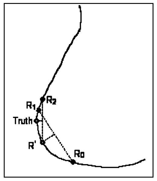
In each mammogram, the nipple location was identified by experienced Mammography Quality Standards Act (MQSA) radiologists. This location was used as the “gold standard” for training the algorithms and evaluating of the computer performance. The radiologist visually inspected the image displayed on a monitor with a graphical user interface and used the windowing function to enhance the breast boundary. The radiologist marked the nipple location by using the cursor. One radiologist estimated the nipple location for all of the images in the visible nipple class. For the invisible nipple class, one radiologist estimated the nipple locations twice, another radiologist estimated the nipple location only once. The “gold standard” was estimated by averaging the radiologists' readings. Since the breast boundary is not a straight line, the averages of the x and y coordinates of two points along the breast boundary generally do not fall on the boundary. An average between two readings was thus estimated as the intersection between the breast boundary and the normal to the midpoint of the line connecting the two readings, as shown in Fig. 1. When the two readings are not too far apart, this method is very close to that obtained by finding their midpoint along the breast boundary. However, this method is less prone to error if the breast boundary points are noisy. Using this averaging method, the average point R′ was first estimated from Radiologist 1's two readings R₀ and R₁, then the “gold standard” was found as the average of point R′ with Radiologist 2's reading R₂.

Fig. 1.

Estimation of “gold standard” for invisible nipple images.

B. Breast boundary detection

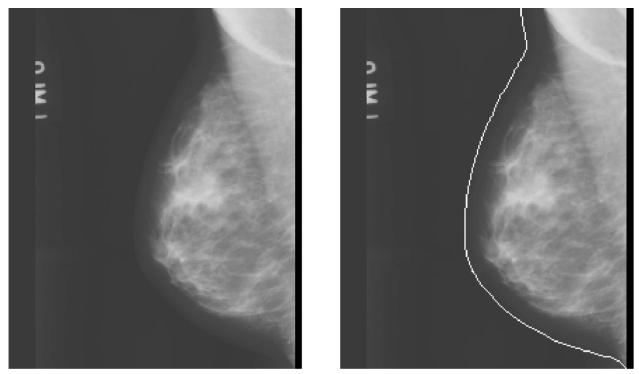
The detection of breast boundary was the first step in our computerized nipple detection algorithm. The breast boundary separated the breast from the surrounding background which included the directly exposed area, the patient identification information, and lead markers. Computerized analysis was then performed only around the breast region after boundary detection. The breast boundary was first identified by a boundary tracking technique. The automated boundary tracking technique previously developed^10,11 was modified to improve its performance. The breast boundary was identified by a gradient-based method as follows. The background of the image was estimated initially by searching for the largest background peak from the gray level histogram of the image. A preliminary edge was found by a horizontal line-by-line gradient analysis starting from the top to the bottom of the image. The criterion used in detecting the edge points was the steepness of the gradient along the horizontal direction. The steeper the gradient, the greater the likelihood that an edge existed at that corresponding location. The preliminary edge served as a guide for a more accurate tracking algorithm that was subsequently applied. The tracking of the breast boundary started from approximately the middle of the breast image and moved upward and downward along the boundary. The direction to search for a new edge point was guided by the previously tracked edge points. The edge location was determined by searching for the maximum gradient along the gray level profile normal to the tracking direction. Because the boundary tracking was guided by the preliminary edge and the previously detected edge points, it could steer around the breast boundary and was less prone to diversion by noise and artifacts. After upward and downward tracking was finished, the tracked edges were smoothed to remove noisy fluctuations. A simple linear interpolation was used to connect the edge points so that a continuous breast boundary was found. An example of the tracked breast boundary is shown in Figs. 2(a) and 2(b).

Fig. 2.

(a) A mammogram from our image database; (b) the image superimposed with the detected breast boundary.

C. Limiting the nipple search region

If the breast is properly positioned for imaging, almost all the nipples will be located along or close to the breast boundary. Our nipple search was performed within a small window of 9×9 pixels along the breast boundary, with the center of the search window located at the boundary point.

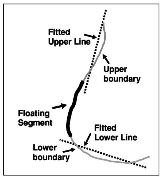
Defining a small search region along the breast boundary would reduce the chance that jagged breast borders from noise and artifacts would result in false positive nipple identification. We designed a geometric convergence analysis to estimate a nipple search region where the nipple would most likely be located. In an ideal situation, the nipple was located close to the boundary, approximately in the middle region of the breast for CC view and in the lower region for MLO view. As shown in Fig. 3, in the geometric convergence analysis, a floating segment containing 20% of boundary points was first placed at the middle of the breast boundary. The floating segment separated the boundary into an upper and a lower boundary segment. Two lines were then fitted to the boundary points in the upper and lower segments and the goodness-of-fit of the two lines was estimated by the sum of squares of the deviations between the fitted line and the boundary points. The convergence region was finally determined by moving the floating segment along the boundary until the deviation of the fitted lines from the breast boundary was minimized. The two fitted lines intersected the anterior region of the breast boundary at two points. The boundary region between these two points was defined as the nipple search region.

Fig. 3.

Defining a limited nipple search region by geometric convergence analysis.

D. Nipple detection

1. Nipple search along breast boundary

After automated breast boundary detection, the breast boundary was smoothed to reduce small jagged fluctuations. From our analysis, we observed that there were sudden and distinct gray level changes in pixels close to the nipple for most of the mammograms with visible nipples. The direction of the breast boundary also had a sudden and distinct change when a convex nipple shape occurred along the breast boundary. In order to identify the location where these changes occurred, we constructed two smoothed intensity curves corresponding to the inner and outer intensity profiles and the curvature curve along the boundary, as defined in Eqs. (1)-(3). The curves were plotted against boundary point B_x, where x=1, …, n_B,n_B represented the total number of boundary points:

• Inner intensity curve:

  $$C_I\left(B_x\right)=\frac{1}{n_I}\underset{k=1}{\overset{n_I}{\Sigma }}f\left(k\right),k\in R_I,B_x\in \text{Breast Boundary},$$ (1)
• Outer intensity curve:

  $$C_O\left(B_x\right)=\frac{1}{n_O}\underset{k=1}{\overset{n_O}{\Sigma }}f\left(k\right),k\in R_O,B_x\in \text{Breast Boundary},$$ (2)
• Curvature curve:

  $$D\left(B_x\right)=\frac{1}{n_D}\underset{k=1}{\overset{n_D}{\Sigma }}d\left(k\right),k\in R_D,B_x\in \text{Breast Boundary},$$ (3)

where R_I, R_O, and R_D were pixels within a 5×5 window of the inner profile, the outer profile, and 5 neighborhood boundary points, respectively. Each window was centered laterally at the current boundary point B_x. n_I, n_O, and n_D represented the number of pixels within each window. f(k) and d(k) were the gray level of the kth pixel within the window and the curvature at the kth boundary point, respectively. On the boundary point B_x, the first derivative, or the gradient, was estimated as the tangent T_x to the breast boundary at B_x. The curvature at B_x was the derivative of the gradient curve,¹² which represented the direction change of the tangent at boundary point B_x.

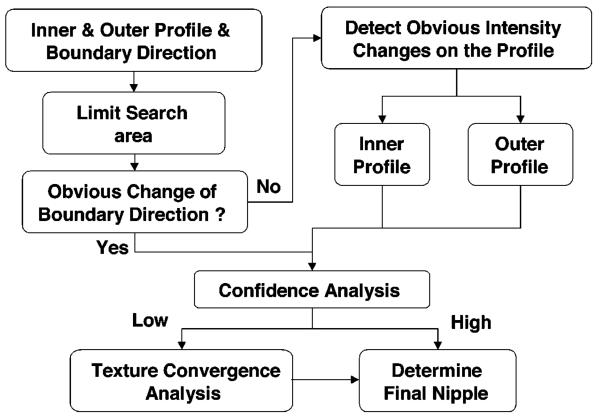
Figure 4 shows the nipple search scheme based on the boundary features. Nipple search was performed taking into account three situations in which the nipple exhibited different characteristics. First, a nipple shape was projected along the breast boundary. In the second and third situations, a nipple intensity profile could be identified inside or outside of the breast boundary. The details are described below.

Fig. 4.

Schematic of the automated nipple search method.

Within the limited nipple search region, the first step was to detect if there was a sudden and distinct change in the boundary direction, which indicated a convex nipple shape outside of the boundary. The convex nipple could be detected by searching for the sharpest peak on the curvature curve. The peak feature p_R of every peak along the curve was calculated as the ratio of the peak height to the peak width. The sharpest peak was identified as the maximum of the peak features p_R. If the maximum peak feature p_R was larger than a predefined threshold, then there was a convex nipple shape depicted on the boundary. The nipple location was identified as the peak point, N_convex, of the sharpest peak on the curvature curve. The threshold was determined using the training data set.

If no convex nipple could be found (i.e., no peak feature larger than the threshold), then the nipple search was performed by searching for obvious intensity changes along the inner and outer intensity profiles separately. Two peak features of the intensity curve were used to detect obvious intensity changes. The first peak feature p_R was estimated as the ratio of the peak height to the peak width. The second peak feature p_H was the peak height normalized to the sum of all the curve heights. If both p_R and p_H for a given peak were larger than the predefined thresholds, then it was an obvious intensity peak. The thresholds were again determined using the training data set. The most obvious intensity change was identified by the maximum p_H if more than one obvious intensity peaks were found along the intensity curve. If obvious intensity changes were found along both the inner and outer intensity curves, the potential nipple location N_intensity was identified at the peak point of the intensity peak with maximum p_H on each curve. If the two maximum intensity peaks located on the inner and outer intensity curves were very close (defined as within 1 cm in our study), then the nipple location N_intensity was identified to be the average of these two peak points. The average location was taken as the intercept of the breast boundary with the normal to the midpoint of the line connecting the two peak points. If these two peak points were not close, then the nipple location N_intensity was determined as the maximum peak on the outer intensity profile because the outer intensity profile generally was less affected by structural noises. The nipple candidate N_convex or N_intensity identified by this rule-based method is referred to as Nipple 1.

Due to the image quality, artifacts, or dense area near the breast border, the computer may identify a jagged breast boundary, which would lead to false detection of the nipple. To reduce the false detections, the identified candidate nipple location N_convex or N_intensity was subjected to a confidence analysis. If there were several cosinelike peaks of similar size in the curvature curve or the inner intensity curve, it indicated that the breast boundary was jagged or there were dense tissues near the breast boundary, respectively. The confidence of the identified nipple was therefore set to low. The confidence was also set to low if the candidate nipple location N_convex or N_intensity was null because the peak features were less than the predefined thresholds. In this situation, the nipple could not be found by the breast-boundary-based method described above and texture convergence analysis would be used as described next.

2. Nipple identification using texture convergence analysis

If the confidence of the rule-based nipple detection was set to low, a flow field based convergence analysis was initiated to estimate the nipple location based on the convergence of texture pattern of glandular tissues or ducts towards the nipple. The fibroglandular tissues or ducts appeared as oriented and flowlike textural pattern on the mammograms. With the assumption that there exists a dominant orientation at each pixel within a texture pattern, an “orientation image” can be computed from the gray level mammogram using least mean squares estimation based on Rao's optimal solution.¹³ Let g_x(u,v) and g_y(u,v) represent the gradients at pixel (u,v) in the image. The gradient magnitude is computed as $G_{u,v}=\sqrt{g_x^2(u,v)+g_y^2(u,v)}$, and the gradient orientation is computed as θ_u,v=arctan(g_y(u,v)/g_x(u,v)). Assuming that the dominant orientation in a N×N local neighborhood centered at pixel (i, j) is ϕ(i, j), the sum-of-squares S can be computed as

$$S=\underset{u=1}{\overset{N}{\Sigma }}\underset{v=1}{\overset{N}{\Sigma }}{G}_{u,v}^2{\cos }^2({\theta }_{u,v}-\varphi (i,j)),$$ (4)

where S is the sum of the squared gradient magnitudes projected along a direction ϕ(i, j) in this neighborhood. ϕ(i, j) is the dominant orientation if S is the maximum. The maximum of S with respect to ϕ(i, j) can be found by solving the equation (dS/dϕ(i, j))=0,

$$\frac{\mathit{dS}}{d\varphi (i,j)}=2\underset{u=1}{\overset{N}{\Sigma }}\underset{v=1}{\overset{N}{\Sigma }}{G}_{u,v}^2\cos ({\theta }_{u,v}-\varphi (i,j))\sin ({\theta }_{u,v}-\varphi (i,j)).$$ (5)

Thus, the dominant orientation ϕ(i, j) can be estimated as

$$\begin{array}{cc}\hfill \varphi (i,j)& =\frac{1}{2}{\tan }^{-1}\left(\frac{{\Sigma }_{u=1}^N{\Sigma }_{v=1}^N{G}_{u,v}^2\sin 2{\theta }_{u,v}}{{\Sigma }_{u=1}^N{\Sigma }_{v=1}^N{G}_{u,v}^2\cos 2{\theta }_{u,v}}\right)\hfill \\ \hfill & =\frac{1}{2}{\tan }^{-1}\left(\frac{{\Sigma }_{u=1}^N{\Sigma }_{v=1}^{N}2g_x(u,v)g_y(u,v)}{{\Sigma }_{u=1}^N{\Sigma }_{v=1}^N(g_x^2(u,v)-g_y^2(u,v))}\right).\hfill \end{array}$$ (6)

Dense breasts generally exhibit more textural structures than fatty breasts on the mammograms. However, due to the presence of noise, the estimated local texture orientation may not always be correct. A low-pass filter can be used to find the local orientation that varies slowly in the local neighborhood. Before performing low-pass filtering, the orientation image was converted into a continuous vector field¹³ defined as follows:

$${ϴ}_x(i,j)=\cos \left(2\varphi (i,j)\right)$$ (7)

and

$${ϴ}_y(i,j)=\sin \left(2\varphi (i,j)\right).$$ (8)

The low-pass filtering was performed by averaging of ϴ_x(i, j) and ϴ_y(i, j) in a local window with a size of 5×5 pixels, yielding ${ϴ}_x^{\prime }(i,j)$, and ${ϴ}_y^{\prime }(i,j)$, respectively, as the smoothed continuous vector field. The smoothed local orientation at (i, j) can then be computed as

$$O(i,j)=\frac{1}{2}{\tan }^{-1}\left(\frac{{ϴ}_y^{\prime }(i,j)}{{ϴ}_x^{\prime }(i,j)}\right).$$ (9)

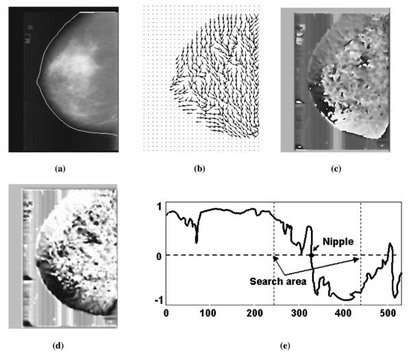
Figure 5 shows an example of a computed orientation field superimposed on the original mammogram. The nipple location was indicated by the convergence of the estimated texture orientation. The following steps were used for the detection of the convergence of the texture orientation:

• (1) Convert the smoothed orientation image into a continuous vector field:¹⁴

  $$O_x(i,j)=\cos \left(O(i,j)\right).$$ (10)
• (2) Identify the points of O_x in the inner profile region and then average to a 1D profile:

  $$C_{Ox}\left(B_x\right)=\frac{1}{n_I}\underset{k=1}{\overset{n_I}{\Sigma }}{O}_x\left(k\right),k\in R_I,B_x\in \text{Breast Boundary},$$ (11)

  where n_I is the number of points within the local window represented by R_I. In our study, the size of R_I is 5 35. For simplicity, the index k is used to identify a point in R_I, replacing the indices (i, j).

• (3) Detect the transition point of C_Ox by searching for the maximum gradient of C_Ox as shown in Fig. 5(e). A large gradient of the C_Ox indicated the convergence of the texture orientation which led to the location of nipple. A candidate nipple location O_x (Nipple2) was found if the maximum gradient was larger than a predefined threshold T_I. The threshold T_I was determined using the training data set.

Fig. 5.

An example of texture orientation field convergence analysis. (a) Original image superimposed with the detected breast boundary, (b) texture orientation field, (c) continuous orientation field O, (d) cosine component of continuous field O_x, (e) profile of O_x identified along the breast boundary.

In addition to the maximum gradient location, another indication of a nipple candidate is an approximately circular cluster of pixels with high orientation field strength. Because some of the nipples exhibited a convex shape, there would be a bright dot occupying several pixels on the image of orientation field O as shown in Fig. 5(c). Such bright dot indicated a candidate nipple, which we will refer to as Nipple3 in the following discussions. Note that, although the rule-based method could detect convex nipple location by searching for the maximum curvature of the breast boundary as described in Sec. II D 1, the confidence of the identified nipple might be set to low because of jagged breast boundary. In such a case, alternative nipple locations would need to be considered.

3. Determination of the final nipple location

After rule-based nipple detection along the boundary profile, and the convergence analysis using texture orientation field, three candidate nipple locations were obtained, as described above. Nipple1 was found by the rule-based method, Nipple2 was found by the change in the orientation projection O_x, and Nipple3 was found by the orientation field O. If the confidence of Nipple1 was set to high, the final nipple location was determined by Nipple1. Otherwise, the following rules were used to determine the final nipple location:

Situation 1: Both Nipple2 and Nipple3 could be detected by texture convergence analysis

• (1) If the distances between the three candidate nipples were all smaller than 0.5 cm (6 pixels), then the final nipple location was determined by Nipple1.

• (2) If the distance between Nipple1 and Nipple2 was larger than 0.5 cm and the distance between Nipple1 and Nipple3 was smaller than 0.5 cm, then the final nipple location was determined by Nipple1.

• (3) If the distance between Nipple1 and Nipple3 was larger than 0.5 cm and the distance between Nipple1 and Nipple2 was smaller than 0.5 cm, then the final nipple location was determined by Nipple1.

• (4) If the distance between Nipple2 and Nipple3 was less than 0.5 cm but the distances from Nipple1 to both Nipple2 and Nipple3 were larger than 0.5 cm, then the final nipple location was determined by Nipple3.

• (5) If the distances between every two of the three candidate nipples were larger than 0.5 cm, it indicated that the confidence of nipple detection using texture convergence analysis was low, then the final nipple location was determined by Nipple1. However, if Nipple3 was less than 0.5 cm from the breast boundary, it indicated that Nipple3 had higher confidence because nipple projection had a good convex shape, then Nipple3 was determined as the final nipple location.

Situation 2: only Nipple2 could be detected by texture convergence analysis

• (1) If the distance between Nipple2 and Nipple1 was smaller than 0.5 cm, then the final nipple location was determined by Nipple1.

• (2) If the distance between Nipple2 and Nipple1 was larger than 0.5 cm, then the final nipple location was determined by Nipple2 if the maximum gradient of the 1D inner profile C_Ox of the smoothed continuous orientation field O was larger than another predefined threshold T₂ (T₂>T₁); otherwise the final nipple location was determined by Nipple1. The threshold T₂ was determined using the training data set.

Situation 3: only Nipple3 could be detected by texture convergence analysis

• (1) Similar to Situation 2, if the distance between Nipple3 and Nipple1 was smaller than 0.5 cm, then the final nipple location was determined by Nipple1.

• (2) If the distance between Nipple3 and Nipple1 was larger than 0.5 cm then the final nipple location was determined by Nipple3 if Nipple3 was less than 0.5 cm from the breast boundary; otherwise the final nipple was determined by Nipple1.

III. RESULTS

A. Breast boundary tracking

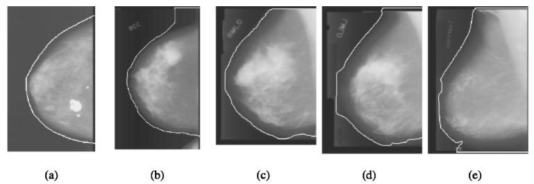
Our breast boundary tracking method was evaluated quantitatively in a previous study.¹⁵ In this study, we applied the program to 744 mammograms. A qualitative performance evaluation of the tracked boundary was performed. Each of the computer tracked breast boundary was rated in three major categories and the “true” boundary was judged visually by an experienced medical physicist. If the boundary was very close to the true boundary it was rated as 0. Borders with a large section of local deviations were rated as 1− and 1+, where + and − indicated if the tracked boundary was outside or inside of the true boundary, respectively. Very poorly tracked borders or total failures were rated as 2− or 2+. Figure 6 shows typical examples of tracked breast boundary rating. The boundary shown in Fig. 6(a) is very closed to the true boundary and rated as 0. The upper section of the boundary was tracked outside the true boundary as shown in Fig. 6(b), which was rated as 1+. The lower section of the boundary was tracked into the breast region as shown in Fig. 6(c), which was rated as 1−. Figure 6 (d) showed a very poorly tracked boundary that was rated as 2−. Figure 6(e) showed an example of failure in the lower part of the boundary tracking that tracked along the edge of the x-ray field and was rated as 2+. Of the 744 mammograms, 89.78% (668/744) of the tracked breast boundaries were rated as 0, 9.81% (73/744) were rated as 1+ or 1−, and 0.67% (5/744) were rated as 2− or 2+. The results showed that the boundaries in most of the mammograms in the data set were tracked very well. Although the boundaries which were rated as 1− and 1+ had local deviations, they were reasonably good to be used for nipple identification as discussed in Sec. IV.

Fig. 6.

Typical examples of tracked breast boundary rating: (a) rating as 0; (b) rating as 1+; (c) rating as 1−; (d) rating as 2−; (e) rating as 2+.

B. Nipple identification

Because the diameters of nipples are larger than 1 cm for most patients, we chose the criterion of correct detection to be a distance of within 1 cm from the computer detected nipple location to the gold standard for evaluating the performance of the computerized nipple identification method. Table I shows the results for computer detected nipple location with an error within 1 cm of the gold standard. For the visible nipple images, the computer identified 89.37% (269/301) of the nipple location within 1 cm (mean =0.34 cm) of the gold standard for the training set, and 92.28% (275/298, mean=0.30 cm) of the nipple location within 1 cm of the gold standard for the test data set. For the invisible nipple images, the computer detected 69.74% (53/76, mean=0.24 cm) of the nipple location within 1 cm of the gold standard for the training data set, and 53.62% (37/69, mean=0.21 cm) of the nipple locations within 1 cm of the gold standard for the test set. The overall performance achieved by the computer in nipple detection including all images with visible or invisible nipple was 85.41% (322/377) and 85.01% (312/367) for the training and test data set, respectively.

Table I.

Performance of the automated nipple detection program. The nipple detection accuracy is quantified as the percentage of images in which the detected nipple location is within 1 cm to the gold standard.

		Number of images	Rule-based method	Rule-based method with texture analysis
Training set	Visible	301	82.39% (248/301)	89.37% (269/301)
	Invisible	76	65.79% (50/76)	69.74% (53/76)
	All	377	79.05% (298/377)	85.41% (322/377)
Test set	Visible	298	89.93% (268/298)	92.28% (275/298)
	Invisible	69	47.83% (33/69)	53.62% (37/69)
	All	367	82.02% (301/367)	85.01% (312/367)

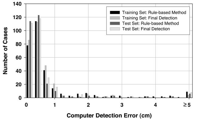
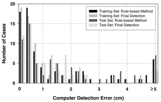
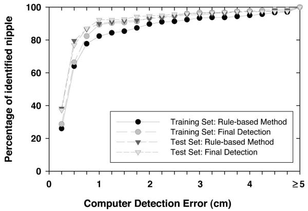
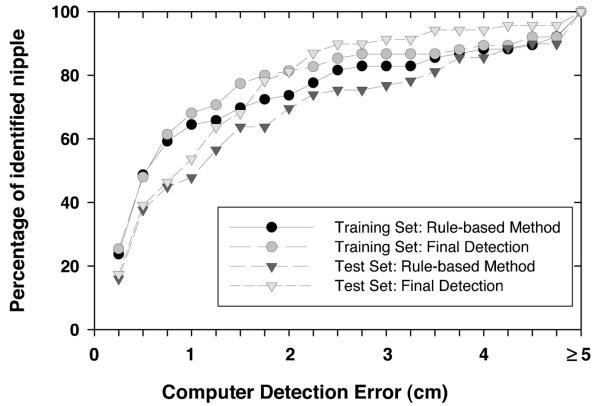
To investigate the usefulness of the texture convergence analysis for nipple identification, we computed the nipple detection results without convergence analysis, in other words, by relying only on Nipple1 location identified by the rule-based method. This results in a simpler detection system, because none of the conditions in Sec. II D 3 are applied. In this situation, 82.39% (248/301) of the visible nipples and 65.79% (50/76) of the invisible nipples in the training data set, and 89.93% (268/298) of the visible nipples and 47.83% (33/69) of the invisible nipples in the test data set could be identified within 1 cm of the gold standard by using the rule-based nipple identification method. The mean errors under these conditions were 0.30 cm, 0.23 cm, 0.28 cm, and 0.18 cm, respectively. For all of the images including visible and invisible nipples, 79.05% (298/377) and 82.02% (301/367) of the nipple locations were identified within 1 cm of the gold standard. The images with errors larger than 1 cm were mainly caused by noise or artifacts along the breast boundary. Figures 7 and 8 show the histograms of the errors for our computerized nipple detection program for visible and invisible nipples, respectively. Figures 9 and 10 show the cumulative percentage of images of which the identified nipple was within a certain distance from the gold standard for visible and invisible nipples, respectively. The computer performances at any detection error threshold can be obtained from these plots.

Fig. 7.

Histogram of computer detection error (Euclidean distance from the detected nipple location to the “gold standard”) for the mammograms in the visible nipple class.

Fig. 8.

Histogram of computer detection error (Euclidean distance from the detected nipple location to the “gold standard”) for the mammograms in the invisible nipple class.

Fig. 9.

The cumulative percentage of identified nipples with a computer detection error (Euclidean distance from the detected nipple location to the “gold standard”) less than or equal to a certain distance for the visible nipple mammograms.

Fig. 10.

The cumulative percentage of identified nipples with a computer detection error (Euclidean distance from the detected nipple location to the “gold standard”) less than or equal to a certain distance for the invisible nipple mammograms.

C. Observer variability for identifying invisible nipples

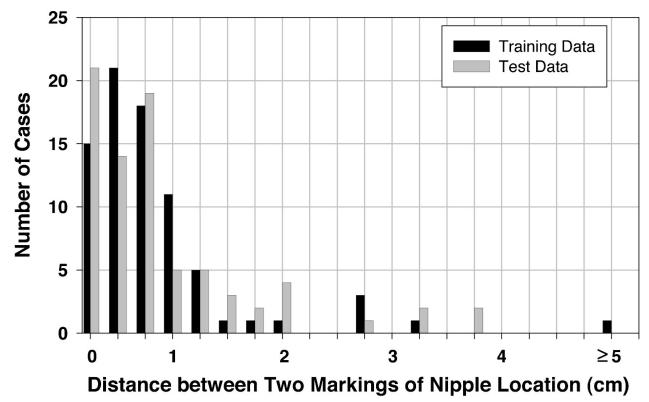
For the nipples that could not be positively identified, i.e., the invisible nipples, an estimated location was given by the radiologists based on visual assessment. The average of estimated nipple locations of two radiologists was used as the “gold standard” to reduce the subjective bias between radiologists. For the training set, if Radiologist 1's first reading, second reading, and the average of these two readings were compared to Radiologist 2's reading, the percentage of images with an agreement within 1 cm between the two estimated nipple locations was 84% (64/76), 79% (60/76), and 83% (63/76), respectively. If Radiologist 1's two readings were compared, the percentage of images with an agreement within 1 cm was 87% (66/76). However, if Radiologist 1's first reading, second reading, the average of these two readings, and Radiologist 2's reading were compared to the averaged “gold standard,” the percentage of images with an agreement within 1 cm was 92% (70/76), 91% (69/76), 93% (71/76), and 99% (75/76), respectively. For the test set under the same conditions, the percentage of images with an agreement within 1 cm was 80% (55/69), 78% (54/69), and 78% (54/69) for the interobserver comparisons, 77% (53/69) for the intraobserver comparison, and 84% (58/69), 90% (62/69), 93% (64/69), and 96% (66/69) if the two radiologists' readings were compared to the averaged “gold standard.” Figure 11 shows the histogram of intraobserver variation in marking the nipple locations by Radiologist 1 for the invisible nipple images in the training and test set.

Fig. 11.

Histogram of the intraobserver variations in marking the nipple locations by Radiologist 1 for the invisible nipple class.

IV. DISCUSSION

In this study, the resolution of the digitized mammograms was reduced to 800 μm×800 μm for identification of the nipple locations both by the radiologists and by the computer. This low resolution was chosen in order to increase the computational efficiency. To verify that this resolution was sufficient for nipple identification, we performed a limited observer study to evaluate the dependence of the nipple visibility on pixel size. Eight full resolution images (50 μm×50 μm) with invisible nipple (classified at 800 μm×800 μm resolution) and one with a very subtle nipple profile were used. The images were subsampled to 100 μm, 200 μm, 400 μm, 600 μm, and 800 μm pixel size. One experienced MQSA radiologist who provided the gold standard described above was asked to visually inspect the nipple location on images of pixel size from 800 μm down to 100 μm individually. The windowing and zooming functions were used in the process of inspection. The observer study indicated that, if a nipple was not visible in a lower resolution image, for example, 800 μm, the nipple still could not be identified confidently by the radiologist on higher resolution images up to 100 μm. This result may be attributed to the fact that the size of the nipple is generally much larger than 800 μ×800 μm. The visibility of the nipple is not limited by the resolution of the image at this pixel size. Most of the invisible nipples were caused by their nearly flat profiles, by the noise along the breast boundary, or by masking of the nipple behind dense tissue due to improper positioning. The smoothing with a box filter reduces the noise which may actually improve the visibility of objects that are not resolution-limited. The visibility of the nipples therefore was not improved by using higher resolution images.

The nipple identification method in this study assumes that most nipples are projected within 1 cm of the breast boundary on the mammogram. In our data set, based on radiologist's marking of nipple locations, we rejected 5 mammograms in which the nipple was located far away from the breast boundary due to skin folds or improperly positioned breast for imaging. The cases that contained a big breast exceeding the film area so that no nipple was projected on the mammograms were also rejected. Two experienced radiologists provided the gold standard by visually identifying the nipple location using a computer interface to display and adjust the contrast and brightness of the image. The nipple locations were marked by the radiologists at the center of the projected nipple image regardless of the size of the nipples which may vary from invisible to a diameter of larger than 1 cm. This means that the error of the computer detected nipple location from the gold standard mark would be larger for larger nipples because our computer method identified the nipple by searching along the breast boundary and the detected nipple location was marked at the breast boundary. For the nipples that could not be positively identified, the nipple location was given by radiologists' subjective visual estimation. From the comparison of inter- and intraobserver variability as described in the Results, it can be seen that Radiologist 2 had slightly higher agreement with the gold standard because most of the estimated nipple locations by Radiologist 2 were located between Radiologist 1's two readings. It can also be seen that the agreement between the two radiologists' readings and the “gold standard” was higher for the training set than that for the test set. This is in agreement with the performance achieved by our computer program in detecting nipple locations within 1 cm of the gold standard on the invisible nipple images, which was also higher for the training set (69.74%) than for the test set (53.62%). These results demonstrate that there were large variations in estimating the nipple locations for these diffi-cult cases even by experienced radiologists.

The nipple detection method in this study depends primarily on nipple search along the breast boundary. At this stage, successful identification of the nipple depends on whether the breast boundary is tracked correctly. In the 744 mammograms used in our study, 110 nipples failed to be detected within 1 cm of the gold standard, of which 14.5% (16/110) of the boundary was rated as 1+ or 1−, and 1.8% (2/110) was rated as 2+ or 2−. In the 744 mammograms, the boundaries were rated as 1+ or 1− in 73 mammograms, 78.1% (57/73) of these nipples could be identified within 1 cm of the gold standard. For the 5 mammograms with worst boundary tracking (rated as 2+ or 2−), 60% (3/5) of the nipples still could be identified within 1 cm of the gold standard. Without using texture convergence analysis, 68.5% (50/73) and 60% (3/5) of these nipples were detected within 1 cm of the gold standard, respectively. It indicates that the nipple detection in 7 of the images with boundary rated as 1+ or 1− failed at the stage of rule-based detection but was successful at the stage of texture convergence analysis for the mammograms. However, 2 mammograms with boundary rated as 2+ or 2− could not be correctly identified either by the rule-based method or by the texture convergence method.

There were large variations in the projected nipple images on the mammograms. For the nipples that were projected outside the breast boundary, the nipple should exhibit higher gray levels than the background pixels outside the boundary. For these convex nipples, the tracked breast boundary could depict a nipple shape. The shape depicted on the boundary was unique if no noise, such as fingerprint or artifacts on the film, affected the boundary tracking. In such cases,searching for the nipple shape along the boundary could find a reliable nipple location. However, some of the convex nipples had very poor signal-to-noise ratio due to scattered radiation. These mammograms often also had noisy boundary. Both factors could lead to false detection and thus large errors from the gold standard. For the situation when the nipple was projected inside the breast boundary, the detection was complicated by noise. Most of such noise was due to dense tissue structures near the breast boundary. Detecting the gray level changes along the breast boundary could potentially find the true nipple location. However, the false positives were higher in images of dense breasts with prominent structured noise.

For the cases that had low confidence in the detected nipple location by the rule-based method, the computer performed a texture convergence analysis based on the texture orientation of the dense glandular tissues or ducts near the nipple region. The texture feature analysis was found to be useful for improving the accuracy of nipple identification in this study. With our algorithm, 46.18% (139/301) of the visible nipples and 77.63% (59/76) of the invisible nipples in the training data set, and 72.73% (144/298) of the visible nipples and 89.86% (62/69) of the invisible nipples in the test data set could not be identified with high confidence by the rule-based method and the texture feature analysis was invoked. For these cases that had low confidence in the detection of nipple location by the rule-based method, 84.89% (118/139) of the visible nipples and 64.00% (38/59) of the invisible nipples in the training data set, and 85.42% (123/144) of the visible nipples and 55.00% (34/62) of the invisible nipples in the test data set could be identified within 1 cm of the gold standard by using the rule-based method in combination with texture convergence analysis. We applied a paired t-test to the detection errors on the subset of images for which the texture convergence analysis was used. The results indicated that the improvement in the accuracy was statistically significant for the visible nipple images in the training set (p,0.002) and the invisible nipple images in the test set (p,0.005), and did not achieve statistical significance for the visible nipple images in the test set (p.0.87) and the invisible nipple images in the training set (p.0.68).

In our study, the training and test sets were randomly selected from patient files. The results showed that, for the visible nipples, the algorithm performance achieved a higher accuracy (i.e., percentage of the detected nipples within 1 cm of the gold standard) in the test set (92.28%) than in the training set (89.37%). On the other hand, for the invisible nipples, the detection accuracy was higher in the training set (69.74%) than in the test set (53.62%). The different trends in the two nipple groups are most likely caused by sampling bias such that the visible nipple images in the test set were by chance somewhat easier to detect than those in the training set. To estimate the statistical significance of the difference in the algorithm performances between the training set and the test set, the bootstrap method was used to resample the training set 100 times and similarly for the test set. The mean and the standard deviation of the detection accuracy were then estimated from the bootstrap samples for the training set and for the test set. Using these estimated values, the unpaired t-test showed that the differences in the performance of our nipple detection method between the training set and the test set were statistically significant (p,0.0001) for both the visible and the invisible nipple groups. The estimated mean and standard deviation of the detection accuracy estimated from the resampled training and test sets and the corresponding p-values of the unpaired t-test are shown in Table II.

Table II.

The unpaired t-test result which was used to estimate the statistical significance of the difference in the algorithm performances between the training set and the test set. The mean and standard deviation of the detection accuracy were estimated from the resample training and test data set using the bootstrap method.

		Mean	Standard deviation	p-value of unpaired t-test
Visible nipples	Training set	89.34%	1.87%
	Test set	92.36%	1.58%	<0.0001
Invisible nipples	Training set	69.99%	5.06%
	Test set	54.09%	6.09%	<0.0001

Although the performance of our nipple detection method is reasonable, further improvement in its accuracy is needed. One possible method may be first determining whether the breast contains very dense tissues, especially in the region posterior to the nipple, and weight the confidence of the texture convergence analysis accordingly. We will pursue this and other methods to improve the accuracy in future studies.

V. CONCLUSION

Accurate identification of nipple location on mammograms is challenging because of the variations in image quality and in the nipple projections, especially for the nipples that are nearly invisible on the mammograms. In this work, we developed a two-stage computerized nipple identification method to detect or estimate the nipple location. The results demonstrate that the visible nipples can be accurately detected by our computerized image analysis method. The nipple location can be reasonably estimated even if it is invisible. Automatic nipple identification will provide the foundation for multiple image analysis in CAD.

References

- 1.Landis SH, Murray T, Bolden S, Wingo PA. Cancer statistics, 1998. Ca-Cancer J. Clin. 1998;48:6–29. doi: 10.3322/canjclin.48.1.6. [DOI] [PubMed] [Google Scholar]
- 2.Byrne C, Smart CR, Cherk C, Hartmann WH. Survival advantage differences by age: Evaluation of the extended follow-up of the Breast Cancer Detection Demonstration Project. Cancer. 1994;74:301–310. doi: 10.1002/cncr.2820741315. [DOI] [PubMed] [Google Scholar]
- 3.Zuckerman HC. The Role of Mammography in the Diagnosis of Breast Cancer. In: Ariel IM, Cleary JB, editors. Breast Cancer, Diagnosis and Treatment. McGraw–Hill; New York: 1987. [Google Scholar]
- 4.Paquerault S, Petrick N, Chan HP, Sahiner B, Helvie MA. Improvement of computerized mass detection on mammograms: Fusion of two-view information. Med. Phys. 2002;29:238–247. doi: 10.1118/1.1446098. [DOI] [PubMed] [Google Scholar]
- 5.Sahiner B, Chan HP, Hadjiiski LM, Helvie MA, Roubidoux MA, Petrick N. Computerized detection of microcalcifications on mammograms: Improved detection accuracy by combining features extracted from two mammographic views. Chicago, IL: Nov 30, 2003. December 5. [Google Scholar]
- 6.Hadjiiski LM, Chan HP, Sahiner B, Petrick N, Helvie MA. Automated registration of breast lesions in temporal pairs of mammograms for interval change analysis-local affine transformation for improved localization. Med. Phys. 2001;28:1070–1079. doi: 10.1118/1.1376134. [DOI] [PubMed] [Google Scholar]
- 7.Chandrasekhar R, Attikiouzel Y. A simple method for automatically locating the nipple on mammograms. IEEE Trans. Med. Imaging. 1997;16:483–494. doi: 10.1109/42.640738. [DOI] [PubMed] [Google Scholar]
- 8.Mendez AJ, Tahoces PG, Lado MJ, Souto M, Correa JL, Vidal JJ. Automatic detection of breast border and nipple in digital mammograms. Comput. Methods Programs Biomed. 1996;49:253–262. doi: 10.1016/0169-2607(96)01724-5. [DOI] [PubMed] [Google Scholar]
- 9.Yin FF, Giger ML, Doi K, Vyborny CJ, Schmidt RA. Computerized detection of masses in digital mammograms: Automated alignment of breast images and its effect on bilateral-subtraction technique. Med. Phys. 1994;21:445–452. doi: 10.1118/1.597307. [DOI] [PubMed] [Google Scholar]
- 10.Morton AR, Chan HP, Goodsitt MM. Automated model-guided breast segmentation algorithm. Med. Phys. 1996;23:1107–1108. [Google Scholar]
- 11.Goodsitt MM, Chan HP, Liu B, Morton AR, Guru SV, Keshavmurthy S, Petrick N. Classification of compressed breast shape for the design of equalization filters in mammography. Med. Phys. 1998;25:937–948. doi: 10.1118/1.598272. [DOI] [PubMed] [Google Scholar]
- 12.Worring M, Smeulders AWM. Digital curvature estimation. CVGIP: Image Understand. 1993;58:366–382. [Google Scholar]
- 13.Rao AR, Schunck BG. Computing oriented texture fields. CVGIP: Graph. Models Image Process. 1991;53:157–185. [Google Scholar]
- 14.Jain AK, Prabhakar S, Hong L, Pankanti S. Filterbank-based fingerprint matching. IEEE Trans. Image Process. 2000;9:846–859. doi: 10.1109/83.841531. [DOI] [PubMed] [Google Scholar]
- 15.Zhou C, Chan HP, Petrick N, Helvie MA, Goodsitt MM, Sahiner B, Hadjiiski LM. Computerized image analysis: Estimation of breast density on mammograms. Med. Phys. 2001;28:1056–1069. doi: 10.1118/1.1376640. [DOI] [PubMed] [Google Scholar]