Combining information

Abstract

The combination of information from diverse sources is a common task encountered in computational statistics. A popular label for analyses involving the combination of results from independent studies is meta-analysis. The goal of the methodology is to bring together results of different studies, re-analyze the disparate results within the context of their common endpoints, synthesize where possible into a single summary endpoint, increase the sensitivity of the analysis to detect the presence of adverse effects, and provide a quantitative analysis of the phenomenon of interest based on the combined data. This entry discusses some basic methods in meta-analytic calculations, and includes commentary on how to combine or average results from multiple models applied to the same set of data.

A technique seen widely in computational statistics involves the combination of information from diverse sources relating to a similar endpoint. The term meta-analysis is a popular label for analyses involving combination of results from independent studies. The term suggests an effort to incorporate and synthesize information from many associated sources; it was first coined by Glass [1] in an application of combining results across multiple social science studies. The possible goals of a meta-analysis are many and varied. They can include: consolidation of results from independent studies, improved analytic sensitivity to detect the presence of adverse effects, and/or construction of valid inferences on the phenomenon of interest based on the combined data. The result is often an appropriately weighted estimate of the overall effect. For example, it is increasingly difficult for a single, large, well-designed biomedical study to assess definitively the effect(s) of a hazardous stimulus. Rather, many small studies may be performed, wherein quantitative strategies that can synthesize the independent information into a single, well-understood inference will be of great value. To do so, one must generally assume that the different studies are considering equivalent endpoints, and that data derived from them will provide exchangeable information when consolidated. Formally, the following assumptions should be satisfied:

1. All studies/investigations meet basic scientific standards of quality (proper data reporting/collecting, random sampling, avoidance of bias, appropriate ethical considerations, fulfilling quality assurance/QA or quality control/QC guidelines, etc.).

2. All studies provide results on the same quantitative outcome.

3. All studies operate under (essentially) the same conditions.

4. The underlying effect is a fixed effect; i.e., it is non-stochastic and homogeneous across all studies. (This assumption relates to the exchangeability feature mentioned above.) The different studies are expected to exhibit the same effect, given some intervention.

In practice, violations of some of these assumptions may be overcome by modifying the statistical model; e.g., differences in sampling protocols among different studies—violating Assumption 3—may be incorporated via some form of weighting to de-emphasize the contribution of lower-quality studies.

We also make the implicit assumption that results from all relevant studies in the scientific literature are available and accessible for the meta-analysis. Of course, studies that do not exhibit an effect often are less likely to be published, and so this assumption may be suspect. Failure to meet it is called the file drawer problem [2]; it is a form of publication bias [3,4] and if present, can undesirably affect the analysis. Efforts to find solutions to this issue represent a continuing challenge in modern computational statistics [5-7].

Combining P-Values

Perhaps the most well-known and simplest approach to combining information collects together P-values from K ≥ 1 individual, independent studies of the same null hypothesis, H_o, and aggregates the associated statistical inferences into a single, combined P-value. R.A. Fisher gave a basic meta-analytic technique towards this end; a readable exposition is given in [8]. Suppose we observe the P-values P_k, k = 1, …, K. Under H_o, each P_k is distributed as independently uniform on the unit interval, and using this Fisher showed that the transformed quantities −2log(P_k) are each distributed as χ²(2). Since their sum is then χ²(2K), one can combine the independent P-values together into an aggregate statistic: ${\mathrm{X}}_{\mathrm{calc}}^2=-2{\sum }_{\mathrm{k}=1}^{\mathrm{K}}\log (P_{\mathrm{k}})$. The resulting combined P-value is then $P_{+}=\mathrm{P}[{\mathrm{\chi }}^2(2\mathrm{K})\ge {\mathrm{X}}_{\mathrm{calc}}^2]$. Report combined significance if P₊ is less than some pre-determined significance level, α. This approach often is called the inverse χ² method, since it inverts the P-values to construct the combined test statistic. A simple simulation can illustrate the effect: suppose 10,000 samples of K=5 independent P-values are generated from U(0,1) and ${\mathrm{X}}_{\mathrm{calc}}^2$ is determined for each of these samples. A histogram of the resulting collection of 10,000 X² values is displayed in Figure 1, with a χ²(10) density superimposed. Strong similarity between the distributional forms is evident.

Figure 1.

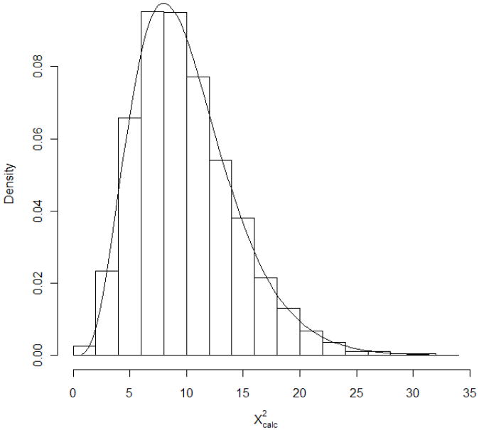
Histogram of ${\mathrm{X}}_{\mathrm{calc}}^2=-2{\sum }_{\mathrm{k}=1}^{\mathrm{K}}\log (P_{\mathrm{k}})$ based on K=5 random P-values sampled 10,000 times. Also superimposed is the p.d.f. of χ²(10).

One can construct alternative methods for combining P-values; for instance, from a set of independent P-values, P₁, P₂, …, P_K, each testing the same H_o, the quantities Φ⁻¹(P_k) are distributed as standard normal: Φ⁻¹(P_k) ~ i.i.d. N(0,1), where Φ⁻¹(·) is the inverse of the standard normal cumulative distribution function. Then, ${\sum }_{\mathrm{k}=1}^{\mathrm{K}}{\mathrm{\Phi }}^{-1}(P_{\mathrm{k}})~\mathrm{N}(0,\mathrm{K})$. Dividing by the corresponding standard deviation, $\sqrt{\mathrm{K}}$, yields yet another standard normal random variable. Thus, the quantity

$${\mathrm{Z}}_{\mathrm{calc}}=\frac{1}{\sqrt{\mathrm{K}}}\sum _{\mathrm{k}=1}^{\mathrm{K}}{\mathrm{\Phi }}^{-1}(P_{\mathrm{k}}),$$

can be used to make combined inferences on H_o. Due to Stouffer et al. [9], this is known as the inverse normal method, or also Stouffer’s method. To combine the P-values into a single aggregate, calculate from Z_calc the lower tail quantity P₊ = Pr[Z ≤ Z_calc], where Z ~ N(0,1). Notice that this is simply P₊ = Φ(Z_calc). As with the inverse χ² method, report combined significance if P₊ is less than a pre-determined level of α.

Historically, the first successful approach to combining P-values involved neither of these two popular methods. Instead, it employed the ordered P-values, denoted as P_[1] ≤ P_[2] ≤ … ≤ P_[K]. Originally proposed by Tippett [10], the method took the smallest P-value, P_[1], and rejected H_o if P_[1] < 1 − (1 − α)^1/K. Wilkinson [11] extended Tippett’s method by using the Lth ordered P-value: reject H_o from the combined data if P_[L] < C_α,K,L, where C_α,K,L is a critical point found using specialized tables [12]. Wilkinson’s extension is more resilient to possible outlying effects than Tippett’s method, since it does not rest on the single lowest P-value; however, it has been seen to exhibit generally poor power and is not often recommended for use [13].

Fisher’s observation that a P-value under H_o is uniformly distributed can motivate a variety of statistical manipulations to combine independent P-values. The few described above represent only the more traditional approaches. For a discussion of some others, see Hedges and Olkin [12] and Loughin [13].

Effect Size Estimation

While useful and simple, combined P-values have drawbacks. By their very nature, P-values are summary measures that may overlook or fail to emphasize relevant differences among the various independent studies [14]. To compensate for potential loss of information, one can calculate directly the size of the effect detected by a significant P-value. For simplicity, suppose we have a simple two-group experiment where the effect of a target stimulus on an experimental treatment group is to be compared with a corresponding control group. For data recorded on a continuous scale, the simplest way to index the effect of the stimulus is to take the difference in observed mean responses between the two groups. When combining information over two such independent studies, it is common to standardize the difference in means by scaling inversely to its standard deviation. Championed by Cohen [15], this is known as a standardized mean difference, which for use in meta-analysis is often called an effect size [16,17].

Formally, consider a series of independent two-sample studies. Model each observation Y_ijk as the sum of an unknown group mean μ_i and an experimental error term ε_ijk: Y_ijk = μ_i + ε_ijk, where i = C (control group), T (target group); j = 1, …, J studies, and k = 1, …, N_ij replicates per study. (The indexing can be extended to include a stratification variable, if present; see [18].) We assume that the additive error terms are independently normally distributed, each with mean 0, and with standard deviations, σ_j > 0, that may vary across studies but remain constant between the two groups in a particular study. Under this model, each effect size is measured via the standardized mean difference

$${\mathrm{d}}_{\mathrm{j}}=\frac{{\mathrm{\phi }}_{\mathrm{j}}({\overline{\mathrm{Y}}}_{\mathrm{T}\mathrm{j}}-{\overline{\mathrm{Y}}}_{\mathrm{C}\mathrm{j}})}{{\mathrm{s}}_{\mathrm{j}}},$$ (1)

where Y̅_ij is the sample mean of the N_ij observations in the jth study (i = C, T), s_j is the pooled standard deviation

$${\mathrm{s}}_{\mathrm{j}}=\sqrt{\frac{({\mathrm{N}}_{\mathrm{Tj}}-1){\mathrm{s}}_{\mathrm{Tj}}^2+({\mathrm{N}}_{\mathrm{Cj}}-1){\mathrm{s}}_{\mathrm{Cj}}^2}{{\mathrm{N}}_{\mathrm{Tj}}+{\mathrm{N}}_{\mathrm{Cj}}-2}}$$

using the corresponding per-study sample standard deviations s_ij, and φ_j is a adjustment factor to correct for bias in small samples:

$${\mathrm{\phi }}_{\mathrm{j}}=1-\frac{3}{4({\mathrm{N}}_{\mathrm{Tj}}+{\mathrm{N}}_{\mathrm{Cj}}-2)-1}.$$

We combine the individual effect sizes in (1) over the J independent studies by weighting each effect size inversely to its estimated variance, Var[d_j]: the weights are w_j = 1/Var[d_j]. A large-sample approximation for these variances that operates well when the samples sizes, N_ij, are roughly equal and are at least 10 for all i and j is [12]

$$\mathrm{Var}[{\mathrm{d}}_{\mathrm{j}}]\approx \frac{{\mathrm{N}}_{\mathrm{Tj}}+{\mathrm{N}}_{\mathrm{Cj}}}{{\mathrm{N}}_{\mathrm{Tj}}{\mathrm{N}}_{\mathrm{Cj}}}+\frac{{\mathrm{d}}_{\mathrm{j}}^2}{2({\mathrm{N}}_{\mathrm{Tj}}+{\mathrm{N}}_{\mathrm{Cj}})}.$$

With these, the weighted averages are

$${\overline{\mathrm{d}}}_{+}=\frac{\sum _{\mathrm{j}=1}^{\mathrm{J}}{\mathrm{w}}_{\mathrm{j}}{\mathrm{d}}_{\mathrm{j}}}{\sum _{\mathrm{j}=1}^{\mathrm{J}}{\mathrm{w}}_{\mathrm{j}}}.$$ (2)

Standard practice traditionally views a combined effect size as minimal (or ‘none’) if in absolute value it is near zero, as ‘small’ if it is near d = 0.2, as ‘medium’ if it is near d = 0.5, as ‘large’ if it is near d = 0.8, and as ‘very large’ if it exceeds 1.0. To assess this statistically, we find the standard error of d̅₊ as $\mathit{se}\left[{\overline{\mathrm{d}}}_{+}\right]=1/\sqrt{{\sum }_{\mathrm{j}=1}^{\mathrm{J}}{\mathrm{w}}_{\mathrm{j}}}$, and build a 1 − α confidence interval on the true effect size. Simplest is the large-sample ‘Wald’ interval d̅₊ ± z_α/2se[d̅₊], with critical point ${\mathrm{z}}_{\mathrm{\alpha }/2}={\mathrm{\Phi }}^{-1}(1-\frac{\mathrm{\alpha }}{2})$.

Example: Manganese Toxicity

In a study of pollution risk, Ashraf and Jaffar [19] reported on metal concentrations in scalp hair of males exposed to industrial plant emissions in Pakistan. For purposes of comparison and control, hair concentrations were also determined from an unexposed urban population (i = C). Of interest was whether exposed individuals (i = T) exhibited increased metal concentrations in their scalp hair, and if so, how this can be quantified via effect size calculations. The study was conducted for a variety of pollutants; for simplicity, we consider a single outcome: manganese concentration (mg/kg, dry weight) in scalp hair. Among six ostensibly homogenous male cohorts (the ‘studies’), the sample sizes, observed mean concentrations, and sample variances were found as given in Table 1. (Note in the table that the sample sizes are all large enough with these data to validate use of the large-sample approximation for d̅₊.) Observed differences in the mean scalp concentrations range from about 1 to over 4 mg/kg across the 6 cohorts. In addition, sample variances differed by less than a factor of 2 for all cohorts except the first and, perhaps more importantly, the variances were not consistently higher in one group compared to the other across the six cohorts.

Table 1.

Sample sizes, sample means, and sample variances for Manganese Toxicity data, where outcomes were measured as manganese concentration (mg/kg, dry weight) in scalp hair [19].

Cohort, j:	1	2	3	4	5	6
i = C (Controls)
NCj	18	17	22	19	12	18
Y̅Cj	3.50	3.70	4.50	4.00	5.56	4.85
${\mathrm{s}}_{\mathrm{Cj}}^2$	2.43	14.06	4.41	12.25	9.99	4.54
i = T (Exposed)
NTj	16	14	23	26	24	18
Y̅Tj	4.63	6.66	6.46	5.82	9.95	6.30
${\mathrm{s}}_{\mathrm{Tj}}^2$	5.57	12.74	8.24	9.73	18.58	5.76

The per-cohort effect sizes, d_j, based on these data can be computed as d₁ = 0.558, d₂ = 0.785, d₃ = 0.763, d₄ = 0.544, d₅ = 1.080, and d₆ = 0.625. That is, for all cohorts the exposure effect leads to increased manganese concentrations in the T-group relative to the C-group (since all d_js are positive), ranging from an increase of 0.558 standard deviations for cohort 1 to an increase of over one standard deviation for cohort 5. To determine a combined effect size, we calculate the inverse-variance weights as w₁ = 8.154, w₂ = 7.133, w₃ = 10.482, w₄ = 10.595, w₅ = 7.082, and w₆ = 8.581.

From these values, one finds using (2) that

$${\overline{\mathrm{d}}}_{+}=\frac{(8.154)(0.588)+\cdots +(8.581)(0.625)}{8.154+\cdots +8.581}=0.710.$$

For a 95% confidence interval, calculate

$$s{e}^2\left[{\overline{\mathrm{d}}}_{+}\right]=\frac{1}{8.154+\cdots +8.581}=0.019,$$

with which we find ${\overline{\mathrm{d}}}_{+}\pm {\mathrm{z}}_{0.025}\mathit{se}\left[{\overline{\mathrm{d}}}_{+}\right]=0.71\pm (1.96)\sqrt{0.019}=0.71\pm 0.27$. Overall, a ‘medium-to-large’ combined effect size is indicated with these data: on average, an exposed male has scalp hair manganese concentrations between 0.44 and 0.98 standard deviations larger than an unexposed male.

Assessing homogeneity

The assumption that the underlying effect is fixed and homogeneous (Assumption 4 from above) is critical if pooling effect size calculations are desired. To evaluate homogeneity across studies, the statistic ${\mathrm{Q}}_{\mathrm{calc}}={\sum }_{\mathrm{j}=1}^{\mathrm{J}}{\mathrm{w}}_{\mathrm{j}}{({\mathrm{d}}_{\mathrm{j}}-{\overline{\mathrm{d}}}_{+})}^2$ can be used [20], where as above, w_j = 1/Var[d_j]. Under the null hypothesis of homogeneity across all studies, Q_calc ~ χ²(J−1). Here again, this is a large-sample approximation that operates well when the samples sizes, N_ij, are all roughly equal and are at least 10. For smaller sample sizes the test can lose sensitivity to detect departures from homogeneity, and caution is advised.

Reject homogeneity across studies if the P-value P[χ²(J−1) ≥ Q_calc] is smaller than some pre-determined significance level, α. If study homogeneity is rejected, combination of the effects sizes via (2) is contraindicated since the d_js may no longer estimate a homogeneous quantity. Hardy and Thompson [21] give additional details on use of Q_calc and other tools for assessing homogeneity in a meta-analysis; also see [4] and [22].

Applied to the Manganese Toxicity data in the example above, we find ${\mathrm{Q}}_{\mathrm{calc}}={{\sum }_{\mathrm{j}=1}^6{\mathrm{w}}_{\mathrm{j}}({\mathrm{d}}_{\mathrm{j}}-0.71)}^2=\cdots =1.58$. The corresponding P-value for testing the null hypothesis of homogeneity among cohorts is P[χ²(5) ≥ 1.58] = 0.90, and we conclude that no significant heterogeneity exists for this endpoint among the different cohorts. The calculation and reporting of a combined effect size here is validated.

Informative Weighting

Taken broadly, an ‘effect size’ can be any valid quantification of the effect, change, or impact under study [16], not just the difference in sample means employed above. Thus, e.g., we might use estimated coefficients from a regression analysis, correlation coefficients, potency estimators from a bioassay, etc. For any such measure of effect, the approach used in (2) corresponds to a more general, weighted averaging strategy to produce a combined estimator. Equation (2) uses ‘informative’ weights based on inverse variances. Generalizing this approach, suppose an effect of interest is measured by some unknown parameter ξ, with estimators ξ̂_k found from a series of independent, homogeneous studies, k = 1, …, K. Assume that a set of weights, w_k, can be derived such that larger values of w_k indicate greater information/value/assurance in the quality of ξ̂_k. A combined estimator of ξ is then

$$\overline{\mathrm{\xi }}=\frac{\sum _{\mathrm{k}=1}^{\mathrm{K}}{\mathrm{w}}_{\mathrm{k}}{\widehat{\mathrm{\xi }}}_{\mathrm{k}}}{\sum _{\mathrm{k}\mathrm{=}1}^{\mathrm{K}}{\mathrm{w}}_{\mathrm{k}}}$$ (3)

with standard error $\mathit{se}[\overline{\mathrm{\xi }}]=1/\sqrt{{\sum }_{\mathrm{k}=1}^{\mathrm{K}}{\mathrm{w}}_{\mathrm{k}}}$. If the ξ̂_ks are distributed as approximately normal, then an approximate 1 − α ‘Wald’ interval on the common value of ξ is ξ̅±z_α/2se[ξ̅]. Indeed, even if the ξ̂_ks are not close to normal, for large K the averaging effect in (3) may still imbue approximate normality to ξ̅, and hence the Wald interval may still be approximately valid. For cases where approximate normality is difficult to achieve, use of bootstrap resampling methods can be useful in constructing confidence limits on ξ [23].

A common relationship often employed in these settings relates the information in a statistical quantity inversely to the variance [24]. Thus, given values for the variances, Var[ξ̂_k], of the individual estimators in (3), an ‘informative’ choice for the weights is the reciprocal (or ‘inverse’) variances: w_k = 1/Var[ξ̂_k]. This corresponds to the approach we applied in Equation (2). More generally, inverse-variance weighting is a popular technique for combining independent, homogeneous information into a single summary measure. It was described in early reports by Birge [25] and Cochran [20]; also see Hall [26].

Discussion: Combining information across models versus across studies

Another area where the effort to combine information is computationally interesting occurs when information is combined across models for a given study, rather than across studies for a given model. That is, we wish to describe an underlying phenomenon observed in a single set of data by combining the results of competing models for the phenomenon. Here again, a type of informative weighting finds popular application. Suppose we have a set of K models, M₁, …, M_K, each of which provides information on a specific, unknown parameter θ. Given only a single available data set, we can calculate a point estimator for θ, such as the maximum likelihood estimator (MLE) θ̂_k, based on fitting the kth model. Then, by defining weights, w_k, that describe the information in or quality of model M_k’s contribution for estimating θ, we can employ the weighted estimator $\overline{\mathrm{\theta }}={\sum }_{\mathrm{k}=1}^{\mathrm{K}}{\mathrm{w}}_{\mathrm{k}}{\widehat{\mathrm{\theta }}}_{\mathrm{k}}$. For the weights, Buckland, et al. [27] suggest

$${\mathrm{w}}_{\mathrm{k}}=\frac{\exp (-I_{\mathrm{k}}/2)}{\sum _{\mathrm{i}=1}^{\mathrm{K}}\exp (-I_{\mathrm{i}}/2)}$$ (4)

where I_k = −2log(L_k) + q_k is an information criterion (IC) measure that gauges the amount of information each model provides for estimating θ, L_k is the value of the statistical likelihood evaluated under model M_k at that model’s MLE, and q_k is an adjustment term that accounts for differential parameterizations across models. This latter quantity is chosen prior to sampling; if q_k is twice the number of parameters in model M_k, I_k will correspond to the popular Akaike Information Criterion (AIC) [28]. Alternatively, if q_k is equal to the number of parameters in model M_k times the natural log of the sample size, I_k will correspond to Schwarz’ Bayesian Information Criterion (BIC) [29]. Other information-based choices for I_k and hence w_k are also possible [30].

Notice that the definition for w_k in (4) automatically forces Σw_k = 1, which is a natural restriction. Since differences in ICs are typically meaningful, some authors replace I_k in (4) with the differences I_k − min_k=1,…,K{ I_k }. Of course, this produces the same set of weights once normalized to sum to 1.

Uses of this sort of weighted model averaging [31,32] has seen rapid development in the early 21st century; examples include optimization of weights for multiple linear regression analyses [33], use of model averaging to estimates risks of arsenic exposures leading to lung cancer [34], and model averaging software with quantal data [35].

References

- 1.Glass GV. Primary, secondary, and meta-analysis of research. Educational Researcher. 1976;5:3–8. [Google Scholar]
- 2.Rosenthal R. The “file drawer problem” and tolerance for null results. Psychological Bulletin. 1979;86:638–641. [Google Scholar]
- 3.Thornton A, Lee P. Publication bias in meta-analysis: its causes and consequences. Journal of Clinical Epidemiology. 2000;53:207–216. doi: 10.1016/s0895-4356(99)00161-4. [DOI] [PubMed] [Google Scholar]
- 4.Tweedie RL. Meta-analysis. In: El-Shaarawi AH, Piegorsch WW, editors. Encyclopedia of Environmetrics. 3. John Wiley & Sons; Chichester: 2002. pp. 1245–1251. [Google Scholar]
- 5.Henmi M, Copas JB, Eguchi S. Confidence intervals and P-values for meta-analysis with publication bias. Biometrics. 2007;63:475–482. doi: 10.1111/j.1541-0420.2006.00705.x. [DOI] [PubMed] [Google Scholar]
- 6.Copas J, Jackson D. A bound for publication bias based on the fraction of unpublished studies. Biometrics. 2004;60:146–153. doi: 10.1111/j.0006-341X.2004.00161.x. [DOI] [PubMed] [Google Scholar]
- 7.Baker R, Jackson D. Using journal impact factors to correct for the publication bias of medical studies. Biometrics. 2006;56:785–792. doi: 10.1111/j.1541-0420.2005.00513.x. [DOI] [PubMed] [Google Scholar]
- 8.Fisher RA. Combining independent tests of significance. American Statistician. 1948;2:30. [Google Scholar]
- 9.Stouffer SA, Suchman EA, DeVinney LC, Star SA, Williams RM., Jr . The American Soldier, Volume I. Adjustment During Army Life. Princeton University Press; Princeton, NJ: 1949. [Google Scholar]
- 10.Tippett LHC. The Methods of Statistics. Williams & Norgate; London: 1931. [Google Scholar]
- 11.Wilkinson B. A statistical consideration in psychological research. Psychological Bulletin. 1951;48:156–158. doi: 10.1037/h0059111. [DOI] [PubMed] [Google Scholar]
- 12.Hedges LV, Olkin I. Statistical Methods for Meta-Analysis. Academic Press; Orlando, FL: 1985. [Google Scholar]
- 13.Loughin TM. A systematic comparison of methods for combining p-values from independent tests. Computational Statistics and Data Analysis. 2004;47:467–485. [Google Scholar]
- 14.Gaver DP, Draper D, Goel PK, Greenhouse JB, Hedges LV, Morris CN, Waternaux C. Combining Information: Statistical Issues and Opportunities for Research. The National Academies Press; Washington, DC: 1992. [Google Scholar]
- 15.Cohen J. Statistical Power Analysis for the Behavioral Sciences. Academic Press; New York: 1969. [Google Scholar]
- 16.Umbach DM. Effect size. In: El-Shaarawi AH, Piegorsch WW, editors. Encyclopedia of Environmetrics. 2. John Wiley & Sons; Chichester: 2002. pp. 629–631. [Google Scholar]
- 17.Piegorsch WW, Bailer AJ. Combining information. In: Melnick EL, Everitt BS, editors. Encyclopedia of Quantitative Risk Analysis and Assessment. 1. John Wiley & Sons; Chichester: 2008. pp. 259–264. [Google Scholar]
- 18.Piegorsch WW, Bailer AJ. Analyzing Environmental Data. John Wiley & Sons; Chichester: 2005. [Google Scholar]
- 19.Ashraf W, Jaffar M. Concentrations of selected metals in scalp hair of an occupationally exposed population segment of Pakistan. International Journal of Environmental Studies. 1997;51:313–321. Section A. [Google Scholar]
- 20.Cochran WG. Problems arising in the analysis of a series of similar experiments. Journal of the Royal Statistical Society. 1937;(Supplement 4):102–118. [Google Scholar]
- 21.Hardy RJ, Thompson SG. Detecting and describing heterogeneity in meta-analysis. Statistics in Medicine. 1998;17:841–856. doi: 10.1002/(sici)1097-0258(19980430)17:8<841::aid-sim781>3.0.co;2-d. [DOI] [PubMed] [Google Scholar]
- 22.Sutton AJ, Higgins JPT. Recent developments in meta-analysis. Statistics in Medicine. 2008;27:625–650. doi: 10.1002/sim.2934. [DOI] [PubMed] [Google Scholar]
- 23.Wood M. Statistical inference using bootstrap confidence intervals. Significance. 2005;1:180–182. [Google Scholar]
- 24.Fisher RA. Theory of statistical estimation. Proceedings of the Cambridge Philosophical Society. 1925;22:700–725. [Google Scholar]
- 25.Birge RT. The calculation of errors by the method of least squares. Physical Review. 1932;16:1–32. [Google Scholar]
- 26.Hall WJ. Efficiency of weighted averages. Journal of Statistical Planning and Inference. 2007;137:3548–3556. [Google Scholar]
- 27.Buckland ST, Burnham KP, Augustin NH. Model selection: An integral part of inference. Biometrics. 1997;53:603–618. [Google Scholar]
- 28.Akaike H. Information theory and an extension of the maximum likelihood principle. In: Petrov BN, Csaki B, editors. Proceedings of the Second International Symposium on Information Theory. Akademiai Kiado; Budapest: 1973. pp. 267–281. [Google Scholar]
- 29.Schwarz G. Estimating the dimension of a model. Annals of Statistics. 1978;6:461–464. [Google Scholar]
- 30.Burnham KP, Anderson DA. Model Selection and Multi-Model Inference: A Practical Information-Theoretic Approach. 2. Springer-Verlag; New York: 2002. [Google Scholar]
- 31.Hoeting JA, Madigan D, Raftery AE, Volinsky CT. Bayesian model averaging: A tutorial. Statistical Science. 1999;14:382–401. corr. vol.15(3), pp. 193-195. [Google Scholar]
- 32.Hjort NL, Claeskens G. Frequentist model averaging. Journal of the American Statistical Association. 2003;98:879–899. [Google Scholar]
- 33.Hansen BE. Least squares model averaging. Econometrica. 2007;75:1175–1189. [Google Scholar]
- 34.Morales KH, Ibrahim JG, Chen C-J, Ryan LM. Bayesian model averaging with applications to benchmark dose estimation for arsenic in drinking water. Journal of the American Statistical Association. 2006;101:9–17. [Google Scholar]
- 35.Wheeler MW, Bailer AJ. Model averaging software for dichotomous dose response risk estimation. Journal of Statistical Software. 2008;26 Art 5. [Google Scholar]
Further Reading List
- Hartung J, Knapp G, Sinha BK. Statistical Meta-Analysis with Applications. John Wiley & Sons; New York: 2008. [Google Scholar]
- Hunter JE, Schmidt FL. Methods of Meta-Analysis: Correcting Error and Bias in Research Findings. 2. Sage Publications; Newbury Park, CA: 2004. [Google Scholar]
- Kulinskaya E, Morgenthaler S, Staudte RG. Meta Analysis: A Guide to Calibrating and Combining Statistical Evidence. John Wiley & Sons; New York: 2008. [Google Scholar]
- Normand S-LT. Meta-analysis software: A comparative review. American Statistician. 1995;49:298–309. [Google Scholar]
- Normand S-LT. Meta-analysis: formulating, evaluating, combining, and reporting. Statistics in Medicine. 1999;18:321–359. doi: 10.1002/(sici)1097-0258(19990215)18:3<321::aid-sim28>3.0.co;2-p. [DOI] [PubMed] [Google Scholar]
- Sutton AJ, Abrams KR, Sheldon TA, Song F. Methods for Meta-Analysis in Medical Research. John Wiley & Sons; New York: 2000. [Google Scholar]
- Stangl DK, Berry DA, editors. Meta-Analysis in Medicine and Health Policy. Marcel Dekker; New York: 2000. [Google Scholar]
- Zaykin DV, Zhivotovsky LA, Czika W, Shao S, Wolfinger RD. Combining p-values in large-scale genomics experiments. Pharmaceutical Statistics. 2007;6:217–226. doi: 10.1002/pst.304. [DOI] [PMC free article] [PubMed] [Google Scholar]