

1. Introduction
This review is on biomolecular NMR data analysis. The context of this discussion is the use of software tools for processing and analyzing NMR data for the ultimate goals of determining the three-dimensional structures of proteins and characterizing other biophysical properties of these macromolecules (such as their internal dynamics).
Since the first publication of a macromolecular solution structure in 1985 [1], the number of structures solved by NMR techniques has risen dramatically, such that at the time of the writing of this review, 8136 NMR structures have been reported accounting for approximately thirteen percent of the structures deposited in the Protein Data Bank. NMR data can provide many possible restraints on the underlying macromolecular structure, such that three-dimensional structures can be determined with reference to inter-atomic distances estimated from NOEs [1] or spin labels [2,3], angular constraints derived from J-couplings [4] or chemical shifts [5,6], hydrogen bonding patterns inferred from amide proton exchange rates [7], and the alignments of bond vectors with respect to the static magnetic field from residual dipolar couplings [8]. Recent techniques have shown success in solving protein structures utilizing chemical shift information alone [9,10]. High resolution NMR data is not solely used for three-dimensional structure determination, however. Often, only limited structural information is necessary and can be ascertained by examining only a subset of the data required for solving the three-dimensional structure. For instance, HN, N, C′, Hα, Cα, Hβ, and Cβ chemical shift data and backbone coupling constant data (3JHN-Hα, 4JHN-Hβ) have been used to delineate secondary structure elements in proteins using a variety of protocols [5,6,11]. Likewise, changes in chemical shift upon ligand or macromolecular binding have been used extensively to map macromolecular binding sites [12,13]. Mapping measurements of this type can also yield key biochemical information, allowing one to measure quantitatively the dissociation and rate constants of binding [14,15] which provide the framework for the method of SAR (structure activity relationships) by NMR [16]. Similarly, correlating changes in chemical shift with a titration in pH has proven to be a robust method for determining the pKa of biochemical moieties either on the surface or buried within folded proteins. Measurements of this kind have been critical in understanding the reaction pathways of enzymes [17].
In addition to structural and biochemical information about macromolecules, NMR has also provided a wealth of dynamics information. Longitudinal (T1, T1ρ) and transverse (T2, T2*) relaxation measurements have been used to characterize overall motions of macromolecules as well as modes of internal motion including backbone librations and side-chain motions of proteins on the timescale of picoseconds to milliseconds[18]. Measurements such as these have been used to measure the microscopic entropy (S) of macromolecules and the change in entropy (ΔS) upon binding effector molecules[19]. Dynamic information at longer timescales (seconds and greater) can be obtained through the monitoring of hydrogen exchange, which in turn has been used to measure the kinetic and thermodynamic properties of protein folding[20].
To summarize the efficacy and versatility of high-resolution NMR as a biomedical tool, the NMR measurement is capable of monitoring a large number of characteristics of biological macromolecules, and can monitor those characteristics in a large number of often overlapping ways.
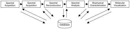
The NMR data processing pipeline consists of several distinct phases: Spectral Acquisition (SQ), the collection of NMR data in the time domain, Spectral Reconstruction (SR), the converting of time-domain data to a spectral representation in the frequency domain, Spectral Analysis (SA), the identification, assignment and characterization of spectral peaks, and Biophysical Characterization (BC), which loosely covers all subsequent data analysis and derivation including structure determination. A fifth analysis component for which software is required (although not technically for data processing) is that of Molecular Visualization (MV), and preceding any NMR experimentation there exists the phase of Sample Preparation (SP).
![]()
There are dozens of software packages available for NMR data handling developed and maintained by both commercial and academic sources. (It would be a true challenge to create a comprehensive list of all available software, and if such a list was to be compiled, it would quickly become out-dated. Interested readers are referred to a few websites which aim to keep such a list current (http://www.spincore.com/nmrinfo/software_s.html and http://www.bmrb.wisc.edu/tools/)). With the possible exception of the CCPN project [21], no one software tool aims to manage the entire NMR data processing pipeline from start to finish. Rather, each tool assists the user in a subset of tasks, usually within the context of only one of the aforementioned processing phases. NMR data is processed using these available tools both in a modular and sequential fashion, such that an individual NMR experiment is typically acquired on a computer connected to the spectrometer hardware, preprocessed for signal enhancement and transformed into a multi-dimensional spectrum on a separate computer system using different software, and then analyzed in both a qualitative and quantitative fashion on a third separate computer. This modular approach has proven very successful and is in fact critical for data analysis at the research level due to the modular nature of NMR experiments themselves. NMR pulse sequences (the core elements of the data acquisition module) are built as modules from pulse sequence components which are designed to manipulate nuclear spins in well-defined ways. By combining the pulse sequence components in various complementary manners, the user acquires several spectra yielding complementary information. The modular approach to data analysis allows the user to preprocess each individual spectrum in a manner appropriate to its acquisition details. Similarly, this modular approach allows the processing, analysis and post-processing of various subsets of data using methods suitable to both the subset of data being analyzed and the information sought by the user. The modular approach has the additional benefit that as the field of biological NMR continues to develop and new methodologies are either added or discontinued, the individual software modules can be efficiently tailored and optimized for the upcoming uses.
The shortfall of current NMR data processing is not that it is done in a modular fashion, but rather that it is done sequentially; and in addition, that it is done sequentially not by choice but rather because of the lack of software integration. The prototypical NMR spectroscopist has a host of information concerning the macromolecule under study (temperature, pH, concentration, macromolecular sequence, pKa) but will set up individual experiments based on past experience rather than any specific information on the sample. This may not seem much of an issue at the acquisition stage, since individual pulse sequences and pulse sequence packages are currently designed with little or no concern about the specifics of the sample. However, this sequential approach becomes a greater detriment as the processing and assignments proceed. The facility of protein assignments, for instance, is predicated on a knowledge of the protein sequence as well as the distribution of observed chemical shifts for the particular nuclei in each amino acid residue. The NMR spectroscopist invariably uses this information; however, its effective organization is lacking in most analysis software packages. Rather, the spectroscopist downloads the protein sequence from one database; retrieves distributions of chemical shifts from another database; corrects for possible isotope shifts from yet another database; and in the end often stores this essential information on a scrap of paper which is kept on the desk for reference.
The redundancy and inefficiency of this policy cannot be overstated. Every new protein requires a new download from the protein sequence database. Every newly designed sample requires new corrections to expected shifts. Each new tabulation is time-consuming and error prone. And since all the data originates from computational operations, such tabulation could easily be automated by a software integration environment and made essentially transparent to the user.
The preceding example discusses only one example of the highly integrated nature of the information required for NMR data processing. If the recompiling of archived information occurred only once or twice throughout the analysis procedure, it could be accomplished with a few carefully written computer scripts. (Such scripts abound throughout the NMR community. The authors of this review provides a free web-based GUI for generating NMR processing scripts at http://sbtools.uchc.edu.) However, NMR information is integrated to such a large extent that a few scripts will not suffice, nor will a large number of scripts. To fully exploit the available information and maximize the efficiency of data analysis, the information must not only be stored in a relational database, but the database must be available at a software level to drive the user’s processing and analysis directions.
The authors of this review are currently building a software integration environment for biomolecular NMR analysis called CONNJUR (http://www.connjur.com). In our efforts to design such a system we have spent much time modeling the processes and data generated and utilized throughout NMR data analysis. This review will focus on four portions of this workflow: preparation and characterization of the sample (SP), time domain data collection on the spectrometer (SQ), conversion of time domain data to the frequency domain (SR), and the assignment of peaks (SA). Discussion of these phases will follow a brief description of a few data types critically important to all NMR data analysis.
2. NMR Data Types
There are hundreds of distinct types of data which can and should be recorded throughout any NMR data analysis workflow. These data types are extremely diverse covering environmental information such as temperature, pressure and humidity; mechanical information regarding the equipment used throughout any steps of NMR data collection, personnel information, status and state information. Readers interested in all such data elements are referred to the websites of CCPN (www.ccpn.ac.uk/ccpn/data-model), the BMRB (www.bmrb.wisc.edu/formats.html), PDB (www.pdb.org) or any of our recent papers [22–24].
While the complete delineation of all possible data elements is beyond the scope of this review, it is worth noting the two most essential data types found in NMR spectroscopy. Those two data types are the nucleus giving rise the NMR signal, and the NMR signal itself.
Nuclei themselves have many properties important for the NMR experiment such as atomic number, atomic mass, spin, and gyromagnetic ratios. But apart from the few properties which must be kept track of, the major data type issue is defining a primary key for each nucleus that exists in a sample, particularly for a sample of macromolecules which themselves may have tens of thousands of distinguishable atoms. This issue will be addressed in the following section on preparing and characterizing the sample.
The NMR signal is of an obviously central importance as it is the measurement itself. From the early days of continuous wave spectroscopy, NMR signals have traditionally been measured and represented as absorption peaks. As such, they have important intrinsic properties such as intensity, chemical shift, linewidth and lineshape. The majority of spectral reconstruction and spectral analysis protocols provide information on each of these properties, while a minority do not [25,26]. Handling data and metadata regarding NMR signals will be addressed in the latter two sections on collecting time domain data, converting time domain data to the frequency domain and analyzing peaks.
3. Prepare and Characterize Sample
In conducting any scientific experiment it is of critical importance to control any causes of variation in the results in order to ensure reproducibility of the experiment within the laboratory environment. It is equally important that environmental variables are recorded and reported to the scientific community to ensure reproducibility by external laboratories. Thus, measurements such as ambient temperature, atmospheric pressure, etc. are often recorded during scientific experimentation, and these measurements are often made in a standard, automated fashion. Along with these standard measurements, standard parameters regarding the staff involved with the data collection, the precise equipment used, reagent brands and/or lots, etc. also need to be recorded. These types of standard recordings are similar within all sub-disciplines of biological research and are equally suitable to standard Laboratory Information Management Systems (LIMS). LIMS for NMR data have recently been proposed [27,28].
With biomolecular NMR samples, additional information regarding the sample conditions is of critical importance – and not simply for the reproducibility of the NMR experiments – but for their design, implementation and for the success of further biomolecular NMR data analysis. In biological NMR experiments, the solvent composition is important for lock settings as well as possible chemical shift standard corrections [29]. Knowing what class of molecule is under study – small molecule, nucleic acid or protein – will help dictate the suite of experiments which can and should be applied. In the case of proteins, the complete chemical structure of the protein(s) under study is a required pre-requisite – both the protein sequence and any potential post-translational modifications.
It is important to note that with NMR studies, it is not enough to know the chemical composition, but also the isotope enrichment of all sample components. In the case of the solvent, the level of isotope enrichment can affect the chemical shift of the solvent which in turn can affect both the lock and chemical shift referencing. In the case of the protein, the pattern of isotope enrichment throughout the protein affects not only the chemical shift, but also the magnitudes of the scalar and dipolar couplings throughout the macromolecule, which in turn affect the relaxation properties and coherence transfer pathways which can be exploited during any individual NMR experiment.
There are four general classes of isotopic labeling schemes: (i) natural abundance, where no isotopic enrichment is used and isotopes are incorporated proportional to their abundance in the natural environment, (ii) uniform labeling, in which an individual isotope is enriched to near 100% abundance, (iii) fractional labeling, in which an individual isotope is added at sub 100% abundance, leading to a sample in which the fractionally enriched isotope is represented in abundance proportional to the fractional enrichment and (iv) site-specific labeling in which particular subsets of atoms within the amino acid residue are selectively enriched with particular isotopes. These four general schemes can be applied for different elements within the same sample. In fact, additional isotope perturbations can be achieved through the mixing of amino acids or amino acid precursors which themselves utilize one of the four above classes of enrichment. This amino-acid, site-specific isotopic labeling is probably most cleverly implemented by the SAIL (stereo-array isotope labeling) approach of isotopic labeling [30], although many other approaches have been used to accomplish various similar goals [31–33].
Information regarding isotopic labeling patterns is not currently utilized by the standard software tools for spectral acquisition, reconstruction and analysis. Rather, the spectroscopist is expected to understand this property of his sample throughout these steps. In simplified cases bearing this burden is no hardship to the spectroscopist. If the sample is 15N labeled, one can run the suite of pulse programs exploiting that nucleus. If the sample is not labeled in this manner, those experiments will fail and the spectroscopist will discover this labeling situation quickly. However, as more specific labeling patterns are attempted, pulse programs which exploit intricate details become available [31], and having a computational representation of the labeling program – one understandable by the software tools – becomes critically important.
For that reason we have recently presented a relational model for protein chemical structure based on the IUPAC recommendations for protein nomenclature [34–36]. The original model covered atom names, chemical bonds, bond angles, torsion angles and chirality [23]. That model was subsequently extended to cover post-translational modification and non-standard amino acids as well as isotopic composition [22]. Fig. 1 illustrates the current status of this model. Further description of the entities and relationships can be found within the original publications.
Figure 1.

Entity-relationship model for the proposed representation for pulse sequences (left-hand side panel) and its associations with the conceptual data model for protein conformation [23] (right-hand side panel). Entities are identified as boxes, relationships between the entities as lines. The key entities for our representation are those of mixings and states, a mixing being a relationship between two states, the input and output states. States and mixings are related to the nuclei with which the magnetization resides and the nuclei involved in the magnetization transfer, respectively. Similarly, states and mixings are also related to the relaxation mechanisms which degrade the signal during those periods. The pulse sequence is defined as a collection of states, ordered by their relationship to mixings. The pulse sequence model is related to the protein data model through two connections: the execution event, corresponding to data acquisition, which ties a pulse sequence to a sample; and the chemical labeling pattern established through the chemical isotope entity.
The importance of keeping track of the sample components in such a model – and by sample components we mean not simply the protein sequence but any modifications and the isotopic labeling expected to be found within the sample under study – is so the computational tools can understand this information and provide additional guidance to the spectroscopist. For instance, in the preceding example where the spectroscopist attempted to collect a 15N HSQC experiment on a natural abundance sample, the spectrometer software could gray-out this selection or otherwise warn the user his choice of experiment was improper for the sample. Similarly, one can envision that if the sample is 15N labeled but not 13C labeled, the spectrometer can automatically turn off 13C decoupling pulses without additional user intervention.
While these particular examples may seem quite trivial when compared to the seemingly large investment of implementing a relational model for isotope labeling, more sophisticated guidance regarding the adaptation of selective pulses when isotope shifts are introduced or the customization of spectral windows with respect to isotope shifts [31] would provide more significant benefits. The largest benefits occur throughout the latter stages of the analysis pipeline and will be expanded upon later in this review.
4. Collect time data on spectrometer
The previous section made the claim that it is important for NMR computational tools to have a robust, internal representation for the sample composition – both chemical bonding networks and isotope labeling patterns. The next two sections will make a similar claim regarding how that information is laid out in the spectral layout – both in the time and frequency domains.
In the time domains, information must be modeled for two important considerations: (i) how the individual points in the spectrum relate to delays within the pulse sequence; and (ii) which chemical shifts and couplings are exploited during the pulse sequence which manifest themselves as the information content of the spectrum (i.e. which nuclear relationships are represented by cross peaks in the frequency spectrum).
The former concern about the time domain layout is important particularly for non-uniform data collection – the situation where in order for a combination in improvements to data collection time, sensitivity and/or resolution, the spectral signal will not be collected uniformly with a set spacing between the time points. Rather, only a subset of the possible evolution times are collected. Such data require more sophisticated processing algorithms than the standard Fourier Transformation to reconstruct a frequency plot, but have additional benefits which outweigh this inconvenience.
4.1 Non-uniform Sampling
4.1.1 Sensitivity
In order to analyze complex NMR data generated from bio-molecules it is desirable to attain high sensitivity and resolution. While NMR is capable of achieving extraordinary resolution for samples in solution, as compared to other spectroscopic techniques, the price that is paid is intrinsically low sensitivity. Recently there have been a number of advances to make improvements in sensitivity, including basic techniques, such as uniform isotopic enrichment of samples with 13C and 15N and using magnetic susceptibility matched NMR tubes to achieve the highest concentration with limited quantities of sample, and technical advances such as higher magnetic field strengths (sensitivity ∝ B03/2), advances in probe design with a factor of 2 improvement in sensitivity, cryogenically cooled NMR probes/preamplifiers with a factor of 3 improvement in sensitivity, and most recently cryogenic probes with higher salt tolerance reducing the noise generated by the sample [37].
4.1.2 The Discrete Fourier transform (DFT)
The discrete Fourier transform (DFT) utilized by Ernst and Anderson [38] revolutionized NMR in the 1970s. In addition to increasing the speed of data collection and allowing efficient signal averaging, DFT NMR was key in the development of multi-dimensional NMR experiments (nD) [39–44]. nD NMR experiments along with high field magnets, sensitive probes, advances in electronics, gradients, and sample preparation have all combined to make NMR a powerful technique for solving the three-dimensional (3D) structure of bio-molecules. A testament to this is that to date around 13% of the structures in the PDB have been determined by NMR. In addition to 3D structure determination, NMR offers a wealth of other uses to study biological samples for biophysical characterization such as probing molecular motions, monitoring protein folding events, binding studies, pH titrations, and many others.
4.1.3 DFT requirements
While the DFT revolutionized NMR, it imposes certain requirements on data collection that make it difficult to achieve a digital resolution comparable to the natural linewidths of the signals, in the interferometric (or indirect) dimension(s) of nD NMR experiments. First, the Nyquist theorem places a lower bound on the sampling rate, or time between points, referred to as the dwell time [45]. The dwell time is inversely proportional to the frequency range of the spectrum. Thus, to avoid aliasing of signals the dwell time must be short enough to cover the frequency range of interest. Secondly, in order to achieve a digital resolution comparable to the natural linewidth, a prerequisite to resolving closely spaced resonances of complex spectra, data must be collected with long acquisition times (tmax). In general data must be collected with acquisition times up to π times the transverse relaxation time (~ 3 × T2) to have a digital resolution comparable to the natural linewidth. Note that setting tmax to a value greater than 1.26 × T2 leads to an improvement in digital resolution, but at a cost of reducing the signal-to-noise ratio (S/N) [46]. Increasing the number of transients (nt) increases the S/N by the square root of nt. Increasing tmax also increases S/N, although to a lesser extent than nt, up to a tmax of 1.26 × T2. Each additional data point collected beyond 1.26 × T2 contributes a greater amount of noise than signal. Time domain data collected to 2× and 3× T2 yield S/N percentages of 96% and 85% respectively, as compared to the maximum S/N at a tmax of 1.26× T2 [46]. Thus the user must decide based on sample concentration, sensitivity of the experiment, instrument time available, and the need for resolution, how large to set tmax. The third constraint imposed by the DFT is that sample points must be collected at uniformly spaced intervals. Thus, to avoid aliasing and achieve digital resolution comparable to the natural linewidths, data must be collected with short time intervals to a tmax equal to ~ 3× T2 at equally spaced intervals.
4.1.4 Time constraints of DFT n-Dimensinal (nD) spectra
The constraints imposed by the DFT have virtually no effect on 1D NMR experiments as the entire FID is collected in milliseconds for biological systems. However, the constraints of the DFT make nD experiments prohibitive in measurement times required to achieve resolution comparable to the natural linewidths. Table 1 shows the expected experiment time in days for 3D and 4D experiments for a 15 and 30 kDa protein assuming tmax set to 0.4, 1.26 and 2.0 times T2 with 4 transients per increment. For 15 and 30 kDa proteins with tmax ~ 1.26× T2, 3D experiment times range from 8.81 to 33.7 days and 2.21 to 10.6 days, respectively. While some of these experiment times fall in an accessible time range for data collection, others clearly do not. Note that these times will increase significantly if additional signal averaging is needed due to low S/N or if additional digital resolution is needed. These time constraints have, to date, kept 4D and higher dimensionality experiments from becoming commonplace; however, the increased resolution afforded by 4D NMR experiments can greatly reduce ambiguity in complex biological systems. From Table 1 a 4D 13C/15N-edited NOESY experiment is expected to take 3019 and 379 days for the 15 and 30 kDa proteins, respectively, with tmax ~ 1.26× T2. Clearly for 4D experiments with uniform sampling tmax must be set to a small factor of T2 to allow the experiment time to be suitable, which will cause the linewidths in each indirect dimension to be broadened significantly as compared to the natural linewidth. Thus, with uniform sampling the true resolution afforded by 3D experiments is rarely achievable and is not possible for 4D experiments in any reasonable amount of time.
Table 1.
Estimated Experimental Times
| tmax | Freq. | 15 kDa Protein (τm ~ 9.3 nsec) | 30 kDa Protein (τm ~ 19.0 nsec) | ||||||
|---|---|---|---|---|---|---|---|---|---|
| A | B | C | D | A | B | C | D | ||
| 0.4× T2 | 600 | 1.28 | 3.40 | 0.89 | 96.6 | 0.32 | 1.07 | 0.22 | 12.1 |
| 0.4× T2 | 900 | 2.08 | 7.70 | 2.00 | 233 | 0.52 | 2.41 | 0.50 | 29.2 |
| 1.26× T2 | 600 | 12.7 | 33.7 | 8.81 | 3019 | 3.20 | 10.6 | 2.21 | 379 |
| 1.26× T2 | 900 | 20.7 | 76.4 | 19.8 | 7288 | 5.18 | 23.9 | 4.96 | 913 |
| 2.0× T2 | 600 | 32.1 | 85.0 | 22.2 | 12074 | 8.06 | 26.7 | 5.57 | 1515 |
| 2.0× T2 | 900 | 52.0 | 193 | 49.9 | 29146 | 13.0 | 60.2 | 12.5 | 3653 |
Expected experiment time, in days, for (A) 3D HNCACB, (B) 3D HNCACB-TROSY, (C) 3D 13C-edited NOESY, and (D) 4D 13C/15N-edited NOESY experiments for a 15 kDa and 30 kDa protein at 600 and 900 MHz. Experiment times were calculated with tmax set to 0.4× T2, 1.26× T2, and 2.0× T2. Experiment times were calculated assuming hyper-complex data along all indirect dimensions, 4 transients per increment, and a time of 1.25 seconds per transient. Sweep widths for 1H, 15N, and 13C were 12, 30, and 70 ppm, respectively. T2 relaxation times and rotational correlation times (τm) were estimated using the program ScheduleTool which can be downloaded from http://sbtools.uchc.edu/nmr/.
These constraints imposed by the DFT are exacerbated at higher field strengths where there is a linear increase in the frequency range for each of the dimensions causing the time interval between points to be shorter. For nD experiments increasing the field strength corresponds to an increase in data collection time by a factor of , where n is the number of dimensions, to achieve the same digital resolution. Note that for certain nuclei (especially 15N, 13C′) the natural linewidths of the signals will increase with field strength due to chemical shift anisotropy (CSA). Increasing the field strength from 600 to 900 MHz could potentially increase the experiment time by 2.25 and 3.38 fold for 3D and 4D experiments, respectively, to keep the same digital resolution at the higher field strength. From Table 1, which allows for increases in R2 rates due to CSA, the experiment times are seen to increase from 1.62 to 2.25 fold for 3D experiments and 2.41 fold for the 4D experiment when increasing from 600 to 900 MHz to attain a digital resolution equal to 1.26× T2 (expected experimental times generated using ScheduleTool: http://sbtools.uchc.edu/nmr).
4.1.5 Linear prediction and spectral aliasing
The limitations imposed by the DFT have been dealt with primarily in two ways, the use of spectral aliasing and linear prediction extrapolation (LP). Reducing the spectral width increases the dwell time between sample points and thus reduces the total number of samples that must be collected to achieve a desired digital resolution; however, reducing the spectral width will cause aliasing. Aliasing of NMR signals is commonplace; for instance, the Nε resonance of arginine has an average chemical shift of 84.7 ppm [47] and is almost always aliased for multidimensional experiments with a HN dimension. In 1H-13C HSQC experiments the resonances are, in general, found near a diagonal as both the 1H and 13C resonances of a bound 1H-13C pair are shifted upfield or downfield together. This allows the 13C spectral width to be reduced 3-fold, aliasing both the upfield and downfield resonances to a region of the spectrum that is largely devoid of resonances [48]. While aliasing a spectrum improves digital resolution it has the disadvantage that there is generally additional overlap in the aliased spectra and the interpretation of the spectra becomes complicated.
Data records in the indirect dimension of nD experiments are often truncated due to instrument time constraints. To eliminate truncation artifacts that arise with short data records, apodization functions are used to force the time domain data to decay to near zero. While this reduces the truncation artifacts it does not help digital resolution. A common approach to increase digital resolution, in cases where tmax was set too short due to time constraints, is to use the early time points and linear prediction (LP) extrapolation to expand the time domain data [49]. LP extrapolation has been employed for years and is still in common use today. In favorable circumstances LP has the ability to increase sensitivity and digital resolution. In non-favorable circumstances, such as noisy data or in aggressive circumstances when data is extrapolated too far, LP can result in false positive peaks [50]. Potentially worse is that LP extrapolation can result in frequency shifts of real signals [50]. This is especially true when the number of sinusoids to be extrapolated is underestimated or the data is noisy. As the sensitivity of biological NMR samples is often limited great care must be used when applying LP extrapolation.
4.1.6 Reduced dimensionality experiments
The limitations imposed by the DFT are well known and have led to a plethora of alternative methods of processing time domain data in an attempt to alleviate the requirements of uniformly collecting data records to long acquisition times in the indirect dimensions. All of these methods have in common the approach of sparse sampling where a reduced set of time domain data points are collected with respect to a full uniformly sampled spectrum. One type of sparse sampling that has gained considerable attention is reduced dimensionality (RD) experiments which rely on coupling the evolution periods of indirect dimensions together, which corresponds to sampling along radial vectors emanating from zero time at various angles [51–55]. Several methods have been developed to process and analyze RD data. Two popular methods are G-matrix Fourier Transform (GFT) [56,57] and Back Projection Reconstruction (BPR) [53,58–61]. These methods have led to additional methods to extract peak information from the projections and to make educated guesses for which radial angles to collect, such as APSY [62–64], EVOCOUP [65], and HIFI [66,67]. While these methods have been invaluable for igniting renewed interest in the use of sparse sampling to reduce the time needed to collect time domain data, they all have the disadvantage of using sparse sampling strategies that are non-random.
4.1.7 Point spread function
Any experiment collected with sparse sampling will have, in addition to random noise, additional artifacts in the spectrum due to the use of sparse sampling. These sampling artifacts originate from a convolution of the point spread function (PSF) for the set of sampled times with the spectrum of the sample [68–70]. The PSF is obtained from the DFT of the sampling scheme where times that are sampled are set to one, and times not sampled are set to zero. Sampling strategies that are regular in nature, such as those used in RD experiments, produce a PSF with strong ridge artifacts leading to spectra with significant sampling artifacts observed as ridges emanating from the signals [68]. Destroying the regularity of the sampling scheme by adding randomness dramatically reduces the ridges in the PSF and hence reduces the sampling artifacts in the spectrum [68]. It has been shown that sampling artifacts originating from the use of sparse sampling are largely dictated by the choice of which points are sampled rather than the method used to process the data; although, the magnitude of the sampling artifacts vary significantly for various processing methods [68]. In general sparse sampling schedules that are random will lead to a PSF with the smallest intensities and hence lead to spectra with the least amount of sampling artifacts. However, such sampling strategies will lead to spectra with weak S/N, especially if tmax is set to a high value, as the mean evolution delay will be large. A good compromise is to use a randomized sample schedule, but one that is skewed to early time points where the signal is strong [69,71–74]. Thus times where the sample is strong (early evolution delays) are sampled more frequently while times where the signal is weak (long evolution delays) are sampled less frequently, in much the same way that the matched filter is used to optimize the S/N in DFT spectra [75]. Indirect dimensions that are constant time are collected randomly with no skewing to early evolution delays. While the sensitivity of an experiment collected with non-uniform sampling (NUS) will be lower than a uniformly sampled experiment, where all the time points are collected, the reduction in S/N is often small compared to the time savings. When factoring in time savings experiments collected with NUS often have a higher sensitivity per unit time as compared to uniform sampling.
4.1.8 Rules of Thumb for Non-Uniform Sampling (NUS) Strategies
As discussed earlier, NUS strategies should have randomness to reduce the amplitude of sampling artifacts and be skewed to early evolution times where the signal is strong to attain high sensitivity per unit time. We have found that a decay rate, for skewing the selected points to early evolution delays, that is 1–2 fold higher than the R2 rates for the expected signals works well. In order to achieve sufficient resolution the tmax along the indirect dimensions should be set sufficiently large, generally 1–2 times the T2 time. A conservative estimate is that approximately one-third of time points need to be collected per indirect dimension, although this is variable due to sample and processing considerations and assumes that the samples fall on an underlying Nyquist grid with a spectral width equal to the desired frequency range. This value can be dramatically smaller in favorable conditions, although for biological samples the sensitivity is usually sufficiently low that a substantial number of sample times must be collected, not just to reduce sampling artifacts, but to achieve the desired S/N. Note that, in general, the amplitude of the sampling artifacts are reduced as the percentage of kept time points is increased. The percentage of NUS points that need to be collected as compared to a uniformly sampled experiment assuming one-third of time points per dimension is given by:
| (1) |
where n = number of dimensions. Thus, the time savings for a 2D, 3D, and 4D NUS experiment, with one-third of the points kept in each dimension, is 3-fold, 9-fold, and 27-fold, respectively. The method used to process the NUS data will dictate whether the time points are collected on an underlying grid (based on the dwell time set by the spectral widths), or whether they are collected at essentially arbitrary times. For NUS strategies using an underlying Nyquist grid, that grid can correspond to a spectral width that is larger than the frequency range of the signals. This increases the effective bandwidth in the indirect dimensions, akin to digital oversampling in the direct dimension, and has been shown to improve spectral quality [70]. This occurs as some of the sampling artifacts arising from NUS are aliases, and increasing the spectral width shifts some of these artifacts out of the spectral region of interest. The guidelines above for choosing the decay rate and the percentage of points kept along each dimension are not suitable for oversampled NUS strategies.
4.1.9 Processing methods suitable for arbitrarily sampled data
Alternatives to GFT and BPR, which can handle NUS data collected in a random manner, with essentially arbitrary evolution times, include “non-uniform Fourier transform” (nuDFT) [76,77], maximum likelihood (MLM) [78,79], Bayesian methods [80,81], multidimensional decomposition (MDD) [82–87], maximum entropy (MaxEnt) [69,88,89], and forward MaxEnt (FM) [90,91]. Each of these methods has strengths and weaknesses and employs a variety of assumptions about the data. nuDFT assumes that times not sampled have zero intensity and utilizes the fast Fourier transform (FFT) to compute the nuDFT by setting the time points not sampled to zero. The main advantage of nuDFT is that it is numerically efficient and utilizes the DFT which gives comfort to spectrocopists who have used the DFT for decades for processing uniformly sampled data. The main disadvantage is that the resulting spectral estimate is a convolution of the PSF for the set of sampled time points with the spectrum of the sample [69,70]. The consequence is that sampling artifacts are quite prominent in nuDFT spectra, and nuDFT spectra often need a post-processing “cleaning” procedure to deconvolve the PSF to make spectra suitable for analysis [92]. In contrast MLM, Bayesian, MDD, and MaxEnt methods will all, to a certain extent, deconvolve the PSF from the resulting frequency spectrum, thus minimizing the sampling artifacts as compared to nuDFT. MLM and Bayesian methods are parametric methods of signal processing and thus assume a model for the signals being analyzed. In general, the data are treated as a sum of exponentially decaying sinusoids. In cases where the S/N is strong, the assumption of an exponentially decaying signal (Lorenzian lineshape) is valid and the number of sinusoids is not underestimated, these methods can achieve tremendous results. However, these methods are prone to false positives and the signals can exhibit “spontaneous splitting” when the data is noisy, the lineshapes are non-Lorenzian, or the estimate of the number of sinusoids is under-estimated. MDD utilizes the less restrictive assumption that all essential features (signals) of an nD spectrum can be described as the sum of a small number of one-dimensional vectors. An advantage of MDD is that it is capable of correctly reproducing the intensities in spectra with high dynamic range (e.g. NOESY spectra) [86,93]. A disadvantage of MDD is that it is not as well developed as other methods, such as MaxEnt, and aspects of MDD, such as the response to noise, are not well understood [70].
4.1.10 Maximum Entropy reconstruction
MaxEnt makes no assumptions about the nature of the signals and its only assumption is that the noise is randomly distributed; thus it is perhaps the most general of the methods suitable for handling NUS data. MaxEnt has several advantages; it is numerically efficient (3D spectra reconstructions can be processed in minutes on desktop computers), makes no assumptions about the signals and thus is generally more robust for determining accurate frequencies of the signals than parametric methods [50], can be applied to very noisy data, and as an inverse method can be used to stably deconvolve linewidth [93] and couplings from spectra allowing increased resolution or “virtual” decoupling [88,94,95]. Detailed descriptions of MaxEnt can be found elsewhere [69,88,89], but in short MaxEnt makes an initial guess of the frequency spectrum (which starts as a blank spectrum). This trial spectrum is inverse Fourier transformed to produce a “mock” FID. The “mock” FID is compared to the experimental data, comparing only the data points from the “mock” FID that were collected. The MaxEnt algorithm analyzes the difference between the “mock” and experimental data and uses that information to generate another trial spectrum. The process is repeated until the inverse DFT of the trial spectrum agrees with the observed experimental data to within the experimental error of the data. The MaxEnt reconstruction determines the spectrum containing the least information, consistent with the measured data. The algorithm implemented in the Rowland NMR Toolkit (http://rnmrtk.uchc.edu/) has an exact solution and follows a descent (each successive “mock” data set is closer to the measured data set).
The main two disadvantages of MaxEnt are that as a non-linear method the signal intensities for high dynamic range spectra are not accurately reproduced, and that there are non-intuitive, adjustable parameters that must be set by the user. While the signal intensities are not accurately reproduced in MaxEnt reconstructions, the peak intensities can be corrected by injecting synthetic sinusoids of known intensity into the time domain data and using the resulting peak amplitudes to create a calibration curve. This method has been utilized with great success for measuring accurate intensities in 15N relaxation spectra which have a high demand on the accuracies on peak intensities [96]. The user adjustable parameters needed for MaxEnt reconstructions are related to the spectrometer sensitivity and the uncertainly (noise level) in the input spectrum. The problem of setting reasonable initial values for these adjustable parameters has been solved using an automatic method of determining their estimates by analyzing the noise in the spectrum and has been implemented in an easy to use web-based script generator [97,98]. The FM method is a special case of the more general MaxEnt where the maximum entropy principle is used to estimate values for the sample points not collected in the NUS data set, while enforcing an exact match between the inverse DFT and the spectral estimate to the samples in the NUS data set [70]. Thus MaxEnt reconstructions and FM are equivalent in the limit when the user adjustable parameter that enforces the agreement between the inverse DFT of the reconstructed spectrum and the measured data has infinite weight. The advantage of FM, or MaxEnt under the conditions where it is equivalent to FM, is that accurate peak intensities are produced; however, these conditions are, in general, not the optimal conditions for analyzing the resulting frequency spectrum.
4.1.11 Data Modeling and File Formats
nD data sets are essentially a series of data blocks, each block representing a free induction decay recorded from the spectrometer. The data sets are intrinsically complicated, as the data may be either complex (for quadrature detection) or real only in any of the dimensions. In addition, some dimensions are convoluted for sensitivity improvements [99] and the data must be rearranged prior to spectral reconstruction. Data structures and the processing required for spectral reconstruction have been thoroughly reviewed by Hoch and Stern [100].
Despite this intrinsic complication of time domain data, the data is typically stored in an abbreviated manner, such that the timing of each point throughout the direct and indirect dimensions is not recorded directly in the file but rather is inferred through the uniform spacing as recorded either by the dwell time or its reciprocal (spectral width). For uniformly sample data, the timing can efficiently be recorded in this manner. However, for non-uniform data sets, the delays in each of the n-dimensions must be stored individually. There are many possible methods of storing non-uniform timing – in our laboratory a secondary correspondence file is produced which maps the “uniformly stored” indirect data points with “non-uniform timings.” No such correspondence list is required for the direct dimension. (As all the data points can be collected without compromising acquisition time, direct dimension data is always collected uniformly).
As a frequency domain spectrum is reconstructed from the time domain data, the data representations will change as certain dimensions convert from time to frequency. This adds additional complexity to the data structure. In addition, most software programs also store a history of the mathematical operations applied to the data to improve sensitivity or resolution (operations such as linear prediction, apodization and zero filling which were discussed earlier). All of these metadata concerning the spectral reconstruction process and the layout of points within the spectral file eventually need to be modeled and stored to facilitate effective software integration.
4.2 Pulse Sequence Model
4.2.1 Introduction
Biological NMR is unparalleled as a spectroscopic technique due to the numerous and intricate ways in which pulsed NMR experiments can be used to probe the vast network of coupled nuclear spin energy states observable in biomolecules. However, while the versatility of NMR methodology is a great gift to the biological spectroscopist, the knowledge-base required to successfully implement NMR techniques on biological samples and to analyze the resulting data can be a substantial impediment to its effective use. Over the past two decades, the number of specialized pulse experiments available to the NMR spectroscopist has become exceedingly large. For instance, the current implementation of Varian’s BioPack contains over one hundred pulse programs, each individual program containing dozens of flags and adjustable parameters designed to produce subtle but distinct changes in the information content extractable from the NMR spectrum. Dozens of additional, novel sequences are published each year. An estimate of the total number of published pulse programs would number in the thousands; an estimate of the total number of useful pulse programs which have not been published could exceed tens of thousands.
In addition to the burden placed on the casual NMR user by the sheer number of pulse sequences available, each individual pulse sequence is intricately complex, being composed of dozens of finely tuned pulses and delays. Several formalisms have been developed to describe the physical basis for these experiments, such as the density matrix [101], product operator [102], coherence transfer [103,104] and coherence flow network [105] formalisms. These formalisms have been of critical importance to both the theoretician in designing NMR pulse sequences to probe for specific information contained within specific coupled networks as well as to the experimentalist in implementing the pulse program and extracting the anticipated spectral information. However, as the number and complexity of pulsed NMR techniques keep growing, expert knowledge of the entire library of pulse experiments currently available is rapidly exceeding the capabilities of even the most gifted NMR spectroscopist. In addition, as the field of NMR spectroscopy continues to grow, the number of users without the training to understand the complexities of the pulse sequence implementations increases. For both these reasons, it is clear that there is the need for a new representation of pulsed experiments, one designed from the perspective of those scientists who wish to utilize NMR methodology without committing themselves to an understanding of the physical basis for how the method works.
The requirements for such a new representation are straightforward. From an information standpoint, the representation should be capable of describing the information content contained within the acquired spectrum when a given pulse experiment is run on a given biological molecule. Pulsed experiments are designed for specific molecular species (for example, proteins or nucleic acids) of specific molecular weights and with specific assumptions as to the magnetic properties of the molecule under investigation (including isotopic labeling, scalar coupling patterns, relaxation behavior and expected chemical shift ranges). Therefore, the representation should be linked to these meta-parameters describing the sample under study. In addition, the representation should adequately describe the ordering of the information obtained – for instance, the dimensionality of the acquired spectrum along with the mixings and couplings which affect the resultant spectrum through changes in peak intensity, multiplicity and frequency. Finally, as any representation is ultimately to be used for communication, either between novice or expert users, the representation is required to be both correct and unambiguous so as to eliminate any potential misinterpretation. An added benefit of such stringent adherence to correctness and elimination of ambiguity, the representation will be of use for communication between computational software tools. For this computational purpose, the representation should be supported by a data model representation capable of cross-referencing the spectrum, the information content contained within the spectrum, along with the meta-parameters describing the assumed chemical structure of the biological sample.
With this in mind, we present here a conceptual data model for describing pulse sequences along with a semi-formal notation which can be used in representing novel sequences. Our proposed notation is based on a commonly-used, ad hoc description referred to throughout the literature as the magnetization transfer pathway. This proposed notation has two somewhat opposing goals. The first is to develop a representation which is broad enough to effectively encompass the description of all pulse sequences currently in use as well as additional sequences which may be developed in the future. The second is to keep the representation sufficiently simple that the NMR community will embrace and use it.
To satisfy the first goal, we have created a representation which is highly extensible, such that certain parameters like relaxation can be represented in various ways depending on the circumstances of the pulse experiment. To satisfy the second goal, we have created a representation whose implementation is flexible, leaving the sequence designer the freedom to choose how he wishes to report the parameters describing his pulse experiment. We believe this representation to be robust and flexible enough for use in modern pulse NMR spectroscopy. This notation and its underlying data model will be useful for communication between NMR spectroscopists at any level of training, as well as for communication between computational tools for the purpose of software integration and/or automation.
The need for a data model of pulse experiments has recently been emphasized by Laue and co-developers of the Collaborative Computing Project for NMR (CCPN) [106]. They present a simplified naming convention for describing the information content of pulse sequences within correspondences and communications, as well as a data model for their nomenclature which has been incorporated into the object model for the CCPN software suite. Our approach differs from that of CCPN in two important respects. Firstly, as the goal of the paper by Fogh et al. [106] was to produce a standardized naming format used primarily for compact, experiment identification, their nomenclature is by necessity over-simplified to allow for succinctness. In contrast, the notation described in this paper captures the full detail of pulsed NMR experiments. Secondly, as the overarching goal of the CCPN project is to retool NMR data analysis by creating a new suite of software tools, they elected to formulate a model about NMR analysis per se, rather than formulate a model of the natural scientific objects and the data about such objects. The notation in this paper takes a different approach, whereby the data itself as it represents the natural phenomena described by the NMR experiments is the driving force for the development of the model the notation incorporates. We believe our conceptual data model and semi-formal notation to be more robust in describing the information content of pulse sequences, being capable of describing more subtle nuances in the data content and organization. A comparison between the two approaches is given.
4.2.2 Theory
The proposed representation of pulsed NMR experiments is essentially a merger of the product operator formalism [102] and what has been loosely termed ‘magnetization transfer pathways.’ Descriptions of the latter are abundant throughout the literature (see [107], for instance), although they are used in an arbitrary and somewhat ad hoc fashion. The common purpose of magnetization transfer pathway descriptions is to delineate the path that nuclear magnetization* follows along the molecular spin network from the beginning of a pulsed experiment through to the end (acquisition) as in the example illustrated below.
The molecular spin network is of primary importance to these descriptions, as they are intended to describe the utility of the pulse experiment in the context of a particular type of molecule. This is in contrast to the coherence transfer formalisms, which are not based with reference to particular molecular systems. It is our goal to formalize the basic description of magnetization transfer pathways by adding rigor regarding which selection mechanisms are operating along the pathway and by adding terms to describe which states along the magnetization pathway are observable and for the relaxation mechanisms which are active along the pathway. The basic premises used at the starting point are three-fold: (1) the common design of all pulsed NMR techniques is to relay magnetization through a series of well-defined states (corresponding to well-defined molecular subsystems) to that of a detectable final state, (2) the various intermediate states may be detectable as well, giving rise to multi-dimensional experiments and (3) selection of magnetization at the intermediate states is obtained in only three ways: chemical shift selection obtained from pulse bandwidth, inter-nuclear coupling selection obtained from tuned delays, and phase selection obtained from chemical shift evolution. (Note that relaxation is not described as a selection mechanism but rather an attenuation of signal.)
In this representation, the basic structure of a pulse sequence is an arbitrary-length series of alternating STATES and MIXINGS with sequences both beginning and ending at a STATE.
![]()
Each STATE is defined by the following information: (1) the NUCLEUS or NUCLEI with which the magnetization currently resides, (2) the relative PHASE of the state (z along the magnetic field axis, x orthogonal to z, and y orthogonal to x), (3) the COUPLING state of potentially coupled nuclei, (4) the RELAXATION mechanisms affecting magnetization at this state and (5) the DURATION of magnetization at this state. Each MIXING is defined by the following information: (1) the COUPLING MECHANISM exploited during this period, (2) the CHEMICAL SHIFT range defined by the flanking pulses, (3) the RELAXATION mechanisms affecting magnetization during this period, and (4) the DURATION of this period. One final piece of information contained in this representation is a list of the states for which magnetization is observable, reflecting the various dimensions in a multidimensional experiment. Table 2 summarizes the information incorporated in this representation as well as the symbolic notation used in for its description.
Table 2.
Summary of information contained in the proposed pulse sequence representation.
| Period | Element | Sub-element | Description | Notation | Example | |
|---|---|---|---|---|---|---|
| State | Nucleus | See below | 1H | |||
| Decoupled Nucleus | Decoupled nuclei listed below in parentheses. | (15N∞) | ||||
| Coupled Nucleus | Coupled nuclei listed above in parentheses. |
|
||||
| Coupling state | Coupling state(s) selected | ↑, ↓ i(nphase), a(ntiphase) | ||||
| Observation | Dimension | Order of increment | 1 | t1, STATES | ||
| Convolution | Phase incr. type | States, RK | ||||
| Phase | Magnetization Phase | x, y, z | 1HZ | |||
| Mixing | Extent | Extent of transfer | p, s or t | →t | ||
| Coupling | Type | Type of coupling | J, NOE | JNH | ||
| Nuclei | Nuclei coupled | NH | ||||
| Coupling Filter | — over coupling |
|
||||
| Both | Nucleus | Element | Element name | H |
|
|
| Isotope Number | Atomic number | 1H | ||||
| Shifts selected (subscript following) | Qualitative selection | C′ | ||||
| Shifts rejected (subscript preceding) | Qualitative null | α | ||||
| Shift offset | Center of excitation | 176ppm | ||||
| Shift Bandwidth | Bandwidth of excitation | 200ppm | ||||
| Shift Null | First excitation null | 56 ppm | ||||
| Shift Profile | Extensible description | SLP | ||||
| Relaxation | Description listed below in brackets | Ad-hoc nomenclature for description of relaxation terms | T1, T2, SQ, MQ | |||
| Duration | Length of period | N/A | [T2] |
The various elements in this representation are modeled in traditional Entity-Relationship (ER) fashion. In this manner, the nuclear parameters are only modeled once, being applicable both for the carrier nuclei in each state as well as the coupled nuclei. Similarly, relaxation descriptions are described only once, but are applicable to both state and mixing entities.
4.2.3 Mixings and Couplings
Mixing in this representation is the mechanism by which magnetization is transferred from one well-defined state to another. All mixings are treated as pairwise interactions between two nuclear magnetization states. These magnetization states can represent different nuclear types or different nuclei of the same type. For instance, polarization transfer uses a J-coupling-mediated mixing to transfer magnetization from one scalar coupled heteronucleus to the other. Even though many separate nuclei in the molecule may be affected by one transfer (all amide groups for instance), these are considered a group of simultaneous pairwise transfers. Similarly, while an NOE mixing may spread magnetization from one proton, A, to several protons, B, C, D and E, this is also to be considered as a group of simultaneous pairwise transfers.
It is useful at this juncture to point out the distinction between the description of NMR pulse sequences and the physics underlying the sequences. Describing NOE transfers as pairwise interactions is by no means an adherence to the two-spin approximation. It is simply a statement that the transfer is only being observed to take place between two spins, regardless of how many spins are actually taking part in the physical transfer. Having represented a collection of NOE interactions as each being individually pairwise, it is still possible to analyze such data as a more complicated multi-spin transfer. However, the end result of any such analysis should explain the apparent pairwise interactions recorded by the pulsed experiment.
Similarly, the role of relaxation in this representation may seem inconsistent. Dipolar relaxation is considered a mixing mechanism if used to generate NOE transfers, but is considered a mechanism of signal attenuation if acting during other periods. Such apparent inconsistency is in fact one of the important features of this representation. While the underlying physics behind dipolar relaxation during an NOE mixing period and a polarization transfer period may be the same, the resultant effect on the qualitative nature of the experiment is completely different. Conveying such a distinction is what this representation is intended to do.
Mixings fall into one of three classifications based on the extend of transfer between states. The first class (t) is full transfer from one nuclear state to another, such that no memory exists in the receptor state as to the history of the magnetization. The second class (s) is partial transfer from one state to another, such that the receptor state is a mixed state of the donor and acceptor nuclei. The third class (p) is a null transfer, in which the donor state simply changes phase by its association described within the mixing. These three cases will be illustrated in the case study.
4.2.4 Relaxation vs. Selection
Relaxation is treated as an incoherent attenuation in the level of magnetization residing at any point along the transfer pathway. It is thus presumed that there is a finite amount of magnetization available for transfer in the first state of the transfer pathway, and the quantity of observable magnetization is steadily attenuated through relaxation mechanisms along the pathway. Thus, the key attribute of relaxation mechanisms is that they result in an incoherent attenuation of signal.
Selection is treated not as a mechanism of signal attenuation but rather as a mechanism for signal separation. Such separation may result in the effective attenuation of unwanted signals. It may be sufficient to separate two signal components and attenuate one of them with pulse field gradients (PFGs) or allow relaxation to selectively attenuate one component over the other. Alternatively, signal separation without attenuation may be the goal of the experiment.
There are three mechanisms of selection built into our description of magnetization pathways. The first mechanism would be imposed by bandwidth restrictions on the pulses. All pulses of measurable duration have a finite frequency bandwidth of excitation. Pulse bandwidth profiles are commonly used as a mechanism for selecting magnetization which is transferred only through a particular nuclear type. A classic example of this would be the HNCO experiment, in which the bandwidth of the carbon pulse is chosen to center on the carbonyl region of the spectrum and null on the alpha region, precisely for the reason of selecting the N→C′ pathway over the N→Cα pathway.
The second selection mechanism is enforced by properly tuned delays which are optimized to allow the desired coupling to evolve at the expense of unwanted couplings. Such an example of this mechanism in action would be that of an HNCO experiment designed to transfer magnetization through the hydrogen-bond. The magnetization pathway is qualitatively the same as that of the classic HNCO experiment, namely N→C′, however when selecting for hydrogen-bonded couplings, the delay is optimized to select for the much weaker three-bond N→C′ coupling across the hydrogen-bond.
The third selection mechanism is achieved by phase selection after chemical shift evolution. With this mechanism, magnetization is allowed to dephase from chemical shift evolution and magnetization only with the proper phase is selected. A simple example of this selection in practice would be the jump-return sequence used for solvent suppression, whereby on-resonance peaks are suppressed and off-resonance peaks are preserved. A more common example would be phase cycling routines in which magnetization with proper phase is added in successive increments, while magnetization with improper phase is subtracted and thereby eliminated.
Pulsed field gradients (PFG) are often considered a means of pathway selection, when used to attenuate undesired signal components which have already been separated using one of the two selection mechanisms listed above. Similarly, relaxation can also be used as a passive mechanism to achieve similar attenuation of previously separated signals. As both PFG and relaxation rely on the three aforementioned mechanisms for signal separation, we chose not to represent either as selection mechanisms in its own right.
While coupling transfer steps are most commonly used to select for the coupled pathway, they can also be used to select against the coupled pathway. In this case, the mixing period is described as selecting for all magnetization states which are excluded by the exploited coupling mechanism. This is illustrated using a TANGO [108] pulse scheme in the case study [Section 4.2.6.5].
4.2.5 Signal Separation
It is emphasized in the preceding section that in this representation, selection mechanisms are defined as methods for separating a combination of signals. Such separation is done either for the purpose of attenuating unwanted pathways or in order to detect multiple pathways in a distinguishable manner. Our treatment of selection focuses mainly on the first purpose, in that our symbolic notation focuses on signals which are selected for (as well as signals which are selected against.) However, when more than one class of signal is selected for, this is accommodated in the representation by simply branching the magnetization transfer pathway such that the observed NMR spectrum is considered a superposition of the multiple pathways. This is illustrated with the carbon-nitrogen dual HSQC in the case study.
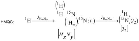
4.2.6 Nitrogen-Hydrogen Correlation Spectroscopy: A Case Study
Two-dimensional, nitrogen-hydrogen correlation spectra are perhaps the most widely used NMR spectra of biological macromolecules. They also comprise a subset of spectra with potentially the largest number of variations in how to acquire them. The basic appearance of the nitrogen-hydrogen correlation spectrum is a two-dimensional plot, with the x-axis containing the proton resonance frequencies, and the y-axis containing nitrogen resonance frequencies. A crosspeak appears at the corresponding intersection of frequencies for each NH group in the macromolecule. While the qualitative level of such information is the same for all such spectra, the principles behind the magnetization transfer as well as the overall appearance of the spectra vary greatly between the several different implementations of this basic experiment. We will use this type of spectroscopy as a case study for demonstrating the utility and practice of our proposed representation.
The majority of NH correlation pulse sequences use an out-and-back strategy, and can be approximately described as:
This description serves to illustrate a few important points regarding the notation. First, the magnetization transfer pathway is an alternating series of STATES and MIXINGS, the states being referred to by the nucleus involved and the mixings being noted as an arrow with the corresponding coupling written above. Second, observable states are labeled according to the Ernst convention for incrementable time periods (for example, t1: being the first incrementable time period described in the model)†. Third, coupled nuclei which are decoupled during a particular state are listed in parentheses below. Treatment of couplings are discussed in more depth in the following section.
As listed in Table 2, nuclei listed in the STATE period are defined by two parameters: the nucleus type and the atomic number. The atomic number parameter is optional; if left out the most-common spin ½ isotope is assumed.
The MIXING period is defined by essentially one parameter, the type of coupling exploited in the transfer. The above example shows the notation for scalar couplings. The coupling is defined not only by the type of coupling, but also the nuclei represented by the coupling as well as the chemical shift range of the nuclei. The chemical shift range is definable in three ways: either qualitatively using conventional notation (in the above example ∞ refers to a hard pulse), semi-quantitatively using a chemical shift range, or rigorously by describing the pulse profile completely. (No notation is defined for the latter, although the common names, durations and intensities of selective pulses could be used.)
Such notation is not meant to imply anything regarding the actual delays used in the experiment as these can be tuned on an experiment-by-experiment basis. As such, no distinction is made regarding subtle differences in coupling constant nor is any indication made as to what the actual coupling constant between the nuclei should be. All that is important is that magnetization is transferred between the two types of nuclei if they share scalar coupling. (Note additionally, that even though relaxation differences between the H→N and N→H transfers may warrant differing delays for these two periods, the coupling exploited is still the same. Similarly, sequences which use relaxation effects [109] or optimal control theory [110] to establish the antiphase magnetization still exploit the same coupling for polarization transfer.)
4.2.6.1 Couplings and Decoupling
The explicit coupling and decoupling of nuclei are accounted for by denoting the coupled nuclei in parentheses either above (active coupling) or below (active decoupling) the ‘observable’ nucleus. If a potentially coupled nucleus is not listed in either location, the coupling is assumed to be active if present. (An example of this would be 13C decoupling during the 15N evolution period. In samples without 13C labeling, the decoupling pulse is not normally included leading to a situation in which the carbon nucleus is neither actively coupled nor actively decoupled. In this situation, the carbon nucleus would be coupled for samples with 13C labeling and uncoupled for samples without.)
The representation of couplings can be illustrated more clearly by examining a TROSY implementation of the HSQC.
While the major incentive for using the TROSY sequence [111] is the decrease in transverse relaxation and subsequent narrower spectral lines, from a magnetization transfer standpoint a second key attribute of the TROSY sequence is the couplings which are selected for. In principle, the TROSY sequence provides a method for selecting either the high- or low-field components of the coupling. Relaxation benefits are realized when selecting the upfield proton component along with the downfield nitrogen component. Our notation uses the up and down arrows to specify the high- and low-field frequency components‡ of a coupling.
When both components appear, the notation i or a is used to distinguish whether the components are in-phase or anti-phase. In the absence of notation, in-phase coupling is assumed. There is an apparent correspondence between this coupling terminology and the coherence which is being evolved as defined by the product operator formalism (HαNy: ↑; HβNy: ↓; HzNy: a; and Ny: i). However, appropriate phase cycling and addition of transients can alter the apparent coupling pattern observed. An example of this would be the sensitivity enhancement sequence [99] in which HzNy evolution results in in-phase coupling.
Although not presented, a similar notation could be developed for distinguishing more complicated multiplet components than encountered here.
4.2.6.2 Inversion Recovery 1H T1 relaxation
The NH correlation experiment is also useful in monitoring amide proton relaxation. A common method for obtaining the relaxation rates is to precede the experiment with an inversion pulse. The following would describe such an experiment using a Bilinear Rotation Decoupling (BIRD) [112] inversion pulse to selectively invert protons which are scalar coupled to 15N nuclei:
where ‘z’ represents longitudinal magnetization, ‘y’ represents transverse magnetization, and ‘c’ represents a scaling of the magnetization imposed by the variable relaxation delay, t1). The preceding description illustrates that longitudinal as well as transverse relaxation can be represented with this notation. Importantly, it also demonstrates that the coupling evolved during the mixing period (in this case JNH) does not necessarily define the flanking nuclear states. In this example, the coupling dictates that only protons coupled to nitrogens are phase inverted (p), without transferring the magnetization through the nitrogen. Only successive mixings (t) transfer the magnetization to the heteronucleus and back again. An additional portion of the notation is added, the convolution state of the observed data can be defined; in this example S refers to States phase incrementation, RK refers to the Rance-Kay mechanism of sensitivity-enhancement [99] and N refers to no convolution. Additional types of convolution can be defined for measuring multiple quantum states (ZQ/DQ)[113], coupling information (J) [42] or combinations of chemical shifts as is done with accordion spectroscopy[114].
4.2.6.3 Alternative mixings and simultaneous acquisition
The 3D NOESY-HSQC is useful to demonstrate how alternative mixing types can be easily represented:
NOE transfers are labeled similarly to polarization transfer. Simultaneous selection of the carbon and nitrogen HSQC is noted by a branch in the pathway.
4.2.6.4 HSQC vs. HMQC
There are two major coherence transfer mechanisms, single and multiple quantum, for generating an NH correlation spectrum. From a product operator standpoint, the HSQC and HMQC sequences differ on the coherence state during evolution, the HSQC evolving single quantum coherence and the HMQC evolving multiple quantum terms [115].
The previous description above using our representation does not distinguish between these two coherence pathways, the reason being that regardless of the coherence order, it is the same scalar coupling which is being exploited for the transfer. However, the qualitative distinction between the two spectra is conveyed once relaxation terms are added to the notation as follow:
Thus, the distinction between HSQC and HMQC spectra becomes primarily one of relaxation mechanisms rather than transfer mechanisms.
However, an additional difference between the single and multiple quantum pulse sequences is the evolution of 1H-1H couplings during t1 in the MQ experiment. This coupling does not evolve during the t1 evolution time of the single quantum (HzNy) experiment, but does evolve in the multiple quantum experiment as the multiple quantum coherence is a mixed state of both 1H and 15N magnetization (HxNy). This representation treats such coherence as that of a mixed state, containing components of both pure states. The notation would be as shown below:
 |
There are a few key points illustrated in the above notation. First, the mixed state is identified as a side-by-side representation of the two pure states. Second, 1H-1H coupling is illustrated by noting 1H coupling above the 1H portion of the mixed state, while 1H-15N decoupling is illustrated by noting 1H decoupling below the 15N portion of the mixed state. Third, the result that t1 captures 15N evolution and not 1H evolution is conveyed by the additional term for the t1 evolution period. In such a manner, many complex evolutions can be described such as 15N+1H which might be found in accordion spectroscopy.
4.2.6.5 Selection Filters
Mixings can be used to select against pathways rather than to select for pathways.
Above is a description of a TANGO (Testing for Adjacent Nuclei with a Gyration Operator) [108] selection of HN magnetization, followed by a gradient to destroy the HN magnetization, followed by a 1H-1H NOESY experiment to effectively filter out amide protons. The use of a selection filter is signified by the bar over the mixing transfer.
4.2.7 Conceptual Data Model
The conceptual data model (CDM) shown in Fig. 1 is semantically equivalent to the proposed notational representation for pulse sequences. The key components relating to pulse sequences are contained within the green box. The central entity of this new model, the pulse sequence (N_PulseSequence), is composed of a series of magnetization states (N_PS_States) as depicted with the semi-formal notation. Each state within the pulse sequence is described with the various attributes outlined in Table 2. Some states within the pulsed experiment are related to each other as being the input and output states of mixing periods. This relationship is delineated as the two-to-many relationship in Fig. 1 between N_PS_States and N_PS_Mixings. As with the N_PS_State entity, the N_PS_Mixing entity records all the relevant attributes outlined in Table 2.
As discussed in the introduction, a key requirement for the conceptual data model is that it relates the information content of the spectrum to the sample meta-parameters. This is accomplished by linking an execution of a pulsed NMR experiment (N_PS_Execution) to a biological sample (B_Sample). This relationship between the pulse sequence and the sample connects the entity-relationship model presented here to that proposed previously for describing the conformation of proteins [23] as shown in Fig. 1. Through this connection, the configuration and execution of a pulse sequence is related to all of the molecular attributes of the sample (chemical shifts, couplings, chemical bonds and molecular structure) which affect the information content and organization of the NMR spectrum.
5. Convert time data to frequency and assign peaks
The layout in the frequency domain is important for the computational tools to understand where the chemical shifts of signals are expected to appear within the spectral matrix – which is critical in order to utilize the isotope labeling patterns for guidance in spectral data collection, reconstruction and analysis.
After NMR data are collected the spectra must be reconstructed and analyzed. There exist a wide variety of different methodologies for processing time domain data and converting it into the frequency domain. The end result requires inspection, visualization, and contextualization in terms of a protein’s amino acid sequence. Thus, one of the major computational challenges in NMR is data visualization, since many spectral data types are multidimensional. In the end, tools such as NMRPipe and the Rowland NMR Toolkit output frequency domain data which can be imported into popular peak analysis and assignment tools.
There are a wide variety of such programs, and the availability of novel tools and algorithms for dealing with visualization of spectral information continues to increase every year. Common tools include NMRDraw, XEASY, CARA, SPARKY, and NMRViewJ [116–119]. We briefly discuss the numerical content of such spectra, as well as the conventional methods for visualization and analysis of common spectra.
5.1 The Numerical Content of FID data
File formats describe multiple free induction decays accumulated from one pulse sequence where variable time delays are present, and it is these “time delays” which yield higher dimensional data. Different variable delay times will select different subsets of nuclei for measurement (individual nuclei precess at different rates). Ultimately, these differences allow for distinction of nuclei in multidimensional spectra of large molecules. Thus, NMR spectra comprise a n-dimensional cube which is a set of numbers which have amplitudes (which yield biophysical information) that are distributed across multi-dimensionally-delayed times.
The conversion of this information to the frequency domain finally yields a hyper-cube of “peaks” - or correlated atomic events induced by the pulse sequence, which can be interpreted in the context of a protein structure or a protein’s dynamics.
5.2 Spectral Processing
Numbers are spread across FID files in numerical chunks or “blocks”. Individual numbers in FIDs have different meaning throughout the processing workflow. Consider a 2D FID, collected in two spectrometer channels. For any given dimension, there are “real” and “imaginary” numbers (corresponding to distinct channels, which might be called “A” and “B”). Once converted to the frequency domain, there are still “real” and “imaginary” components for each fid data point, but those numbers do not correspond to the same semantics. Thus, we find that the imaginary components of frequency domain information can often be discarded after processing is completed.
5.3 Spectral Visualization
A common goal of multidimensional spectral analysis involves the correlation of resonances spanning multiple pulsed NMR spectra. Once time domain data is converted into the frequency domain, information from different spectra are “conceptually” merged (i.e. in the mind of the spectroscopist) in order to build a hyper-dimensional spectral information space [120] which spans different atomic relationships derived from pulse sequences. It is important to remember that n dimensional NMR spectra have n+1 dimensions which are viewed in the frequency domain. For example, a 1D spectrum is viewed in terms of chemical shift vs. amplitude. In 2D experiments, we have three axes, two of which correspond to chemical shifts for the two pulsed nuclei, and a third amplitude.
For precision, it is necessary to work in one or two spectral data axes at a time for many analytical tasks (i.e. peak volume estimation, residue specific peak assignment), but it is ultimately necessary that all such tasks retain their context in terms of other data, and it is this necessity that gives rise to a conceptual hyper-dimensional space in multidimensional NMR.
We briefly consider the different visualization schemes associated with three common spectra, HSQC, HNCA, and NOESY spectra in terms of this hyper-dimensional space. We choose these spectral types not because they are more fundamental then others, but rather, because they require three unique visualization and analysis methods, and are exemplary of the wide variety of data integration tasks necessary for the structural analysis of proteins by NMR. Finally, we integrate these molecular “perspectives” in the context of our broader review, that is, in terms of NMR pulse models, and amino acid sequences (Fig. 2). We summarize this view of the integrated nature of NMR analysis in Fig. 3.
Figure 2.

The various spectra collected in an NMR experiment contain related axes, whose common elements are derived from intersecting nuclei which are targeted by pulse sequences. The figure shows two spectra intersected, a 2D HSQC (right portion) and a 3D HNCA (left portion). The pulse sequence nuclei, which result in the axes in the diagram are shown in terms of the chemical structure (upper right). Correlations for the N-HSQC (blue) and HNCA (maroon) are marked. Visualization of a single HSQC can be done in two dimensions (plus the amplitude dimension, which has the peak amplitude). NH peaks for two residues are illustrated. These two residues are assigned to protein residues by correlating CH strips from an HNCA (right) to their NH dimension, as visualized by the intersecting lines through the NH peaks which end into the vertical planes emerging out of the C axis cross section. The carbon signals (pink circles) can be traced back to the HSQC peaks via these lines - demonstrating the “hyper dimensional” nature of correlation in multidimensional NMR. Higher dimensional NMR pulse sequences thus target both unknown and known information so as to increase information about a molecular system in a correlated and incremental fashion.
Figure 3.

Experimental analyses for NMR span spectral information (bottom left), sequence information (right) and pulse sequence models (upper left). The integration of these artifacts result in a nexus of data which are ultimately utilized to estimate the physical properties of a protein’s conformation and dynamics. See concluding remarks for additional discussion.
5.3.1 N-HSQC
In order to describe the way structural information is gleaned from N-HSQC-NOESY and HNCA spectra, the N-HSQC must be addresed first. The N-HSQC experiment generates a two dimensional spectrum which measures chemical shifts for hydrogen atoms which are directly bonded to nitrogen atoms, and is often used as a molecular signature. Within the concept of the hyperdimensional spectrum, the HSQC experiment is used to correlate the data from HSQC-NOESY and HNCA spectra by providing a shared 2-dimensional plane (HN – N).
Multiple HSQCs can also be collected for a protein in different chemical states, and such data sets can be used to study molecular function. For example, ligand interactions or protein unfolding (i.e. in the presence of a denaturant) have been monitored via integration of signals in multiple HSQC spectra [18,121].
As stated above, each peak in the HSQC represents an N-HN pair. The HSQC does not yield information about which N-HN pair within the protein corresponds to which crosspeak in the spectrum, however. This relationship is determined from HNCA (or HNCA-like) experiments.
It is critical to note that we treat the Nitrogen-HSQC as a reference spectrum because that is convention, but not because of any intrinsic property of the N-HSQC as a reference spectral experiment. The basis for multidimensional data correlation and integration in NMR is not dependant on the HSQC directly, but rather, dependent on the fact that spectra share some subset of common axes, which thus allow their hyperdimensional integration. One could easily pick another pulse sequence as the reference set for an experiment. The fact that HSQCs are relatively simple to collect, and feature individual peaks for each NH containing residue make them a convenent reference point.
5.3.2 HNCA
For peaks obtained in an HSQC we must determine corresponding residues. The HNCA experiments resolve this ambiguity by reproducing a “higher dimensional” HSQC which adds a third dimension for the carbon alpha atom. Measurement of carbon alpha signals by the HNCA pulse enables reconstruction of the chemical shift mappings in the linear sequence of a protein. The HNCA pulse can obtain carbon alpha signals for the i-1 and i residues in each of a protein’s amino acids (at least under ideal conditions). Thus it is often the case that data from the HNCA spectrum is visualized in “strips”, or lined up spectral slices, which correspond to the linear sequence of the protein under study.
It is important to note here that the HNCA is not always sufficient to get a residue’s preceding alpha carbon in HNCA experiments (in some cases, a trailing carbon may not have a strong enough signal, and thus the linear peptide chain of carbon alphas cannot be reconstructed completely), and thus a wide variety of other pulse sequences have been adopted to accomodate less sensitive experimental conditions. Extending this to its logical limit, there are libraries in existence which can specifically target all of the 20 individual amino acids [122,123], which can be used in unique scenarios in which certain pulsed nuclei are unavailable (e.g. with residues such as proline).
5.3.3 HSQC-NOESY
Once we know which residues correspond to which H-N cross peaks, we can determine physical constraints to a protein structure using HSQC-NOESY derived spectral data. NOESY spectra take advantage of the fact that hydrogen nuclei in close proximity to one another have a characteristic, through-space interaction. HSQC-NOESY experiments correlate H-N chemical shifts to through space interactions. HSQC-NOESY data are three dimensional, however it is common to look at the H-H plane of a NOESY experiment in order to analyze these interactions. In the case of NOESY information where peak integration is required, crosspeak boundry definition is an important visualization task.
We thus find that three key spectra which are commonly collected require different visualization schemes, in spite of the fact that those spectra all share a 2-dimensional plane (HN – N).
5.3.4 Visualization of the (n+1)th Dimension: Contour plots
The notion of 2D and 3D spectra obscures the fact that peaks have amplitudes: a “2D” spectrum refers to the number of chemical shift dimensions. There is an additional data dimension which corresponds to the amplitude of peaks in a spectrum. Finer grained analysis of spectra requires visualization of this dimension. Various tasks require one-dimensional visualization of the amplitude dimension.
An example of such analysis is peak integration, which is an important aspect of the process of calculating structural constraints [124]. The integration of peak volumes often requires detailed analysis [125]. Although it is trivial to calculate the volume under a certain line, determination of boundaries for a peak can be error prone. For example, consider the case where two peaks overlap. Integration requires navigation of a spectrum in two dimensions to find a cross peak of interest, and selection of the lower/upper limits of that peak.
A conventional method for visualization of spectra for these tasks involves either contour plotting or coloration. In either case, it is common that the contour (or color) variation correspond to variation in amplitude levels, where as the location on a two-dimensional plane corresponds to chemical shifts.
5.4 Summary
Pulsed NMR yields a wide variety of information. Different spectral data types are visualized in fundamentally different ways. Whereas HNCA-like spectra are often cut into strips, the HSQC is most often visualized as a single grid. Finally, data from NOESY experiments are three dimensional, but often require fine grained, lower dimensional analysis for quantification of individual peak volumes.
6. Conclusions
Fig. 3 illustrates the critical nexus point between the chemical composition of the NMR sample, the pulse programs which extract signals from specific nuclei within the sample, and the layout of the spectra themselves. It is this nexus point which may be considered the conceptual task of peak assignment – establishing a relationship between a subset of nuclei in a sample and a crosspeak within the spectral layout under the conditions of a particular pulse sequence. The chemical connectivities of the sample components dictate which pulse sequences will provide useful information and how they must be configured for optimal results (top right arrow). The pulse sequence in turn dictates how correlative information about the sample will manifest itself in the processed spectrum – thus impacting the spectral reconstruction and spectral analysis workflows (bottom left arrow). The final step – transforming the properties of the NMR signal (or crosspeak) into biophysical constraints on the sample under study is even more broad based, as it encompasses all types of biophysical characterizations possible with NMR, including structure determination, monitoring dynamics, ligand binding, macromolecular complexes, and chemical titrations.
Traditionally, the correlation of these very diverse semantic data types has been done by the NMR spectroscopist with the aid of computational tools. In order for computational tools to improve their usefulness, it is important that the connections between the different semantic data types be made explicit in a machine readible form, rather than being implicit and relying on human inference. We are working towards building a unified, relational data model at this critical nexus point (Fig. 3) so that future computational tools will be better able to assist NMR spectroscopists in their research.
Acknowledgments
This research was funded by US National Institutes of Health grants EB-001496 and GM-083072. The authors wish to thank Drs. George Gray, Heidi J.C. Ellis, Timothy O. Martyn, Jeffrey Hoch, Lorentz Mitschang and Bernd Simon for useful discussions.
Footnotes
In coherence pathway descriptions, the term ‘magnetization’ is usually reserved for single-quantum coherence with ‘coherence’ implying unobservable orders of coherence. Since it is not the intention of this formalism to track the order of coherence, we will use the term ‘magnetization’ to refer to all orders of coherence, observable or not.
Note that the numbering of the observable states reflects nothing more than the order in which they appear in the notation. As our notation is an abstract description of pulsed experiments, such numbering does not reflect either the actual order of incrementation in the executed experiment nor the ordering of data points in the final data matrix.
The high- and low-field components originate from the up and down nuclear spin states, and therefore the two components can be distinguished either by the spin state or the spin energy. However, the relationship between the spin state and energy is complicated by its dependence on the gyromagnetic ratio, which can be either positive or negative, depending on the nucleus. In order to simplify the representation from a user’s perspective, we choose to distinguish based on the more concrete energy state rather than the more theoretical spin state, although it must be emphasized that a pure correspondence and therefore a simple transformation exists between the two representations.
Publisher's Disclaimer: This is a PDF file of an unedited manuscript that has been accepted for publication. As a service to our customers we are providing this early version of the manuscript. The manuscript will undergo copyediting, typesetting, and review of the resulting proof before it is published in its final citable form. Please note that during the production process errors may be discovered which could affect the content, and all legal disclaimers that apply to the journal pertain.
References
- 1.Williamson MP, Havel TF, Wuthrich K. J Mol Biol. 1985;182:295. doi: 10.1016/0022-2836(85)90347-x. [DOI] [PubMed] [Google Scholar]
- 2.Girvin ME, Fillingame RH. Biochemistry. 1995;34:1635. doi: 10.1021/bi00005a020. [DOI] [PubMed] [Google Scholar]
- 3.Gaponenko V, Howarth JW, Columbus L, Gasmi-Seabrook G, Yuan J, Hubbell WL, Rosevear PR. Protein Sci. 2000;9:302. doi: 10.1110/ps.9.2.302. [DOI] [PMC free article] [PubMed] [Google Scholar]
- 4.Karplus M. J Am Chem Soc. 2002;85:2870. [Google Scholar]
- 5.Wang Y, Jardetzky O. Protein Sci. 2002;11:852. doi: 10.1110/ps.3180102. [DOI] [PMC free article] [PubMed] [Google Scholar]
- 6.Wishart DS, Sykes BD, Richards FM. Biochemistry. 1992;31:1647. doi: 10.1021/bi00121a010. [DOI] [PubMed] [Google Scholar]
- 7.Wagner G, Wuthrich K. J Mol Biol. 1982;160:343. doi: 10.1016/0022-2836(82)90180-2. [DOI] [PubMed] [Google Scholar]
- 8.Fowler CA, Tian F, Al-Hashimi HM, Prestegard JH. J Mol Biol. 2000;304:447. doi: 10.1006/jmbi.2000.4199. [DOI] [PubMed] [Google Scholar]
- 9.Shen Y, Lange O, Delaglio F, Rossi P, Aramini JM, Liu G, Eletsky A, Wu Y, Singarapu KK, Lemak A, Ignatchenko A, Arrowsmith CH, Szyperski T, Montelione GT, Baker D, Bax A. Proc Natl Acad Sci USA. 2008;105:4685. doi: 10.1073/pnas.0800256105. [DOI] [PMC free article] [PubMed] [Google Scholar]
- 10.Cavalli A, Salvatella X, Dobson CM, Vendruscolo M. Proc Natl Acad Sci USA. 2007;104:9615. doi: 10.1073/pnas.0610313104. [DOI] [PMC free article] [PubMed] [Google Scholar]
- 11.Cornilescu G, Delaglio F, Bax A. J Biomol NMR. 1999;13:289. doi: 10.1023/a:1008392405740. [DOI] [PubMed] [Google Scholar]
- 12.Marintchev A, Mullen MA, Maciejewski MW, Pan B, Gryk MR, Mullen GP. Nat Struct Biol. 1999;6:884. doi: 10.1038/12347. [DOI] [PubMed] [Google Scholar]
- 13.Gryk MR, Marintchev A, Maciejewski MW, Robertson A, Wilson SH, Mullen GP. Structure. 2002;10:1709. doi: 10.1016/s0969-2126(02)00908-5. [DOI] [PubMed] [Google Scholar]
- 14.Liu D, Prasad R, Wilson SH, DeRose EF, Mullen GP. Biochemistry. 1996;35:6188. doi: 10.1021/bi952656o. [DOI] [PubMed] [Google Scholar]
- 15.Hu HY, Horton JK, Gryk MR, Prasad R, Naron JM, Sun DA, Hecht SM, Wilson SH, Mullen GP. J Biol Chem. 2004;279:39736. doi: 10.1074/jbc.M402842200. [DOI] [PubMed] [Google Scholar]
- 16.Shuker SB, Hajduk PJ, Meadows RP, Fesik SW. Science. 1996;274:1531. doi: 10.1126/science.274.5292.1531. [DOI] [PubMed] [Google Scholar]
- 17.Mullen GP, Antuch W, Maciejewski MW, Prasad R, Wilson SH. Tetrahedron. 1997;53:12057. [Google Scholar]
- 18.Gryk MR, Abseher R, Simon B, Nilges M, Oschkinat H. J Mol Biol. 1998;280:879. doi: 10.1006/jmbi.1998.1731. [DOI] [PubMed] [Google Scholar]
- 19.Yang D, Mok YK, Forman-Kay JD, Farrow NA, Kay LE. J Mol Biol. 1997;272:790. doi: 10.1006/jmbi.1997.1285. [DOI] [PubMed] [Google Scholar]
- 20.Hoang L, Bedard S, Krishna MM, Lin Y, Englander SW. Proc Natl Acad Sci USA. 2002;99:12173. doi: 10.1073/pnas.152439199. [DOI] [PMC free article] [PubMed] [Google Scholar]
- 21.Fogh R, Ionides J, Ulrich E, Boucher W, Vranken W, Linge JP, Habeck M, Rieping W, Bhat TN, Westbrook J, Henrick K, Gilliland G, Berman H, Thornton J, Nilges M, Markley J, Laue E. Nat Struct Biol. 2002;9:416. doi: 10.1038/nsb0602-416. [DOI] [PubMed] [Google Scholar]
- 22.Ellis HJ, Fox-Erlich S, Martyn TO, Gryk MR. ITNG 2006. Las Vegas, NV: 2006. Information Technology: New Generations, 2006; p. 613. [Google Scholar]
- 23.Fox-Erlich S, Martyn TO, Ellis HJ, Gryk MR. Protein Sci. 2004;13:2559. doi: 10.1110/ps.04810204. [DOI] [PMC free article] [PubMed] [Google Scholar]
- 24.Verdi KK, Ellis HJ, Gryk MR. BMC Bioinformatics. 2007;8:31. doi: 10.1186/1471-2105-8-31. [DOI] [PMC free article] [PubMed] [Google Scholar]
- 25.Armstrong GS, Mandelshtam VA, Shaka AJ, Bendiak B. J Magn Reson. 2005;173:160. doi: 10.1016/j.jmr.2004.11.027. [DOI] [PubMed] [Google Scholar]
- 26.Mandelshtam VA, Taylor HS, Shaka AJ. J Magn Reson. 1998;133:304. doi: 10.1006/jmre.1998.1476. [DOI] [PubMed] [Google Scholar]
- 27.Baran MC, Moseley HN, Aramini JM, Bayro MJ, Monleon D, Locke JY, Montelione GT. Proteins. 2006;62:843. doi: 10.1002/prot.20840. [DOI] [PubMed] [Google Scholar]
- 28.Zolnai Z, Lee PT, Li J, Chapman MR, Newman CS, Phillips GN, Jr, Rayment I, Ulrich EL, Volkman BF, Markley JL. J Struct Funct Genomics. 2003;4:11. doi: 10.1023/a:1024684404761. [DOI] [PubMed] [Google Scholar]
- 29.Wishart DS, Bigam CG, Yao J, Abildgaard F, Dyson HJ, Oldfield E, Markley JL, Sykes BD. J Biomol NMR. 1995;6:135. doi: 10.1007/BF00211777. [DOI] [PubMed] [Google Scholar]
- 30.Kainosho M, Torizawa T, Iwashita Y, Terauchi T, Mei Ono A, Guntert P. Nature. 2006;440:52. doi: 10.1038/nature04525. [DOI] [PubMed] [Google Scholar]
- 31.Sweredoski MJ, Donovan KJ, Nguyen BD, Shaka AJ, Baldi P. Bioinformatics. 2007;23:2829. doi: 10.1093/bioinformatics/btm406. [DOI] [PubMed] [Google Scholar]
- 32.Jordan JB, Kovacs H, Wang Y, Mobli M, Luo R, Anklin C, Hoch JC, Kriwacki RW. J Am Chem Soc. 2006;128:9119. doi: 10.1021/ja058587a. [DOI] [PubMed] [Google Scholar]
- 33.Goto NK, Kay LE. Curr Opin Struct Biol. 2000;10:585. doi: 10.1016/s0959-440x(00)00135-4. [DOI] [PubMed] [Google Scholar]
- 34.Markley JL, Bax A, Arata Y, Hilbers CW, Kaptein R, Sykes BD, Wright PE, Wuthrich K. J Mol Biol. 1998;280:933. doi: 10.1006/jmbi.1998.1852. [DOI] [PubMed] [Google Scholar]
- 35.Biochem J. 1984;219:345. [Google Scholar]
- 36.Biochemistry. 1970;9:3471. doi: 10.1021/bi00820a001. [DOI] [PubMed] [Google Scholar]
- 37.Robosky LC, Reily MD, Avizonis D. Anal Bioanal Chem. 2007;387:529. doi: 10.1007/s00216-006-0982-4. [DOI] [PubMed] [Google Scholar]
- 38.Ernst RR, Anderson WA. Review of Scientific Instruments. 1966;37:93. [Google Scholar]
- 39.Jeener J. Ampere International Summer School. Yugoslavia: 1971. [Google Scholar]
- 40.Aue WP, Bartholdi E, Ernst RR. J Chem Phys. 1976;64:2229. [Google Scholar]
- 41.Oschkinat H, Griesinger C, Kraulis PJ, Sorensen OW, Ernst RR, Gronenborn AM, Clore GM. Nature. 1988;332:374. doi: 10.1038/332374a0. [DOI] [PubMed] [Google Scholar]
- 42.Nagayama K, Wuthrich K, Bachmann P, Ernst RR. Biochem Biophys Res Commun. 1977;78:99. doi: 10.1016/0006-291x(77)91226-8. [DOI] [PubMed] [Google Scholar]
- 43.Kay LE, Clore GM, Bax A, Gronenborn AM. Science. 1990;249:411. doi: 10.1126/science.2377896. [DOI] [PubMed] [Google Scholar]
- 44.Marion D, Driscoll PC, Kay LE, Wingfield PT, Bax A, Gronenborn AM, Clore GM. Biochemistry. 1989;28:6150. doi: 10.1021/bi00441a004. [DOI] [PubMed] [Google Scholar]
- 45.Bringham EO. The Fast Fourier Transform. Prentice-Hall, Inc; Englewood Cliffs, New Jersey: 1974. [Google Scholar]
- 46.Rovnyak D, Hoch JC, Stern AS, Wagner G. J Biomol NMR. 2004;30:1. doi: 10.1023/B:JNMR.0000042946.04002.19. [DOI] [PubMed] [Google Scholar]
- 47.Ulrich EL, Akutsu H, Doreleijers JF, Harano Y, Ioannidis YE, Lin J, Livny M, Mading S, Maziuk D, Miller Z, Nakatani E, Schulte CF, Tolmie DE, Kent Wenger R, Yao H, Markley JL. Nuc Acids Res. 2008;36:D402. doi: 10.1093/nar/gkm957. [DOI] [PMC free article] [PubMed] [Google Scholar]
- 48.Bax A, Ikura M, Kay LE, Zhu G. J Magn Reson. 1991;91:174. [Google Scholar]
- 49.Zeng Y, Tang J, Bush CA, Norris JR. J Magn Reson. 1989;83:473. [Google Scholar]
- 50.Stern AS, Li KB, Hoch JC. J Am Chem Soc. 2002;124:1982. doi: 10.1021/ja011669o. [DOI] [PubMed] [Google Scholar]
- 51.Szyperski T, Wider G, Bushweller JH, Wuthrich K. J Am Chem Soc. 1993;116:1601. doi: 10.1007/BF00242481. [DOI] [PubMed] [Google Scholar]
- 52.Malmodin D, Billeter M. Prog Nucl Magn Reson Spectrosc. 2005;46:109. [Google Scholar]
- 53.Kupce E, Freeman R. J Am Chem Soc. 2004;126:6429. doi: 10.1021/ja049432q. [DOI] [PubMed] [Google Scholar]
- 54.Atreya HS, Szyperski T. Methods Enzymol. 2005;394:78. doi: 10.1016/S0076-6879(05)94004-4. [DOI] [PubMed] [Google Scholar]
- 55.Freeman R, Kupce E. J Biomol NMR. 2003;27:101. doi: 10.1023/a:1024960302926. [DOI] [PubMed] [Google Scholar]
- 56.Szyperski T, Atreya HS. Magn Reson Chem. 2006;44:S51. doi: 10.1002/mrc.1817. [DOI] [PubMed] [Google Scholar]
- 57.Kim S, Szyperski T. J Am Chem Soc. 2003;125:1385. doi: 10.1021/ja028197d. [DOI] [PubMed] [Google Scholar]
- 58.Kupce E, Freeman R. J Biomol NMR. 2004;28:391. doi: 10.1023/B:JNMR.0000015421.60023.e5. [DOI] [PubMed] [Google Scholar]
- 59.Kupce E, Freeman R. J Am Chem Soc. 2003;125:13958. doi: 10.1021/ja038297z. [DOI] [PubMed] [Google Scholar]
- 60.Kupce E, Freeman R. J Biomol NMR. 2003;27:383. doi: 10.1023/a:1025819517642. [DOI] [PubMed] [Google Scholar]
- 61.Kupce E, Freeman R. Concept Magn Reson A. 2004;22A:4. [Google Scholar]
- 62.Hiller S, Wider G, Wuthrich K. J Biomol NMR. 2008;42:179. doi: 10.1007/s10858-008-9266-y. [DOI] [PubMed] [Google Scholar]
- 63.Fiorito F, Hiller S, Wider G, Wuthrich K. J Biomol NMR. 2006;35:27. doi: 10.1007/s10858-006-0030-x. [DOI] [PMC free article] [PubMed] [Google Scholar]
- 64.Hiller S, Fiorito F, Wuthrich K, Wider G. Proc Natl Acad Sci USA. 2005;102:10876. doi: 10.1073/pnas.0504818102. [DOI] [PMC free article] [PubMed] [Google Scholar]
- 65.Malmodin D, Billeter M. J Mag Reson. 2005;176:47. doi: 10.1016/j.jmr.2005.05.020. [DOI] [PubMed] [Google Scholar]
- 66.Cornilescu G, Bahrami A, Tonelli M, Markley JL, Eghbalnia HR. J Biomol NMR. 2007;38:341. doi: 10.1007/s10858-007-9173-7. [DOI] [PubMed] [Google Scholar]
- 67.Eghbalnia HR, Bahrami A, Tonelli M, Hallenga K, Markley JL. J Am Chem Soc. 2005;127:12528. doi: 10.1021/ja052120i. [DOI] [PMC free article] [PubMed] [Google Scholar]
- 68.Mobli M, Stern AS, Hoch JC. J Magn Reson. 2006;182:96. doi: 10.1016/j.jmr.2006.06.007. [DOI] [PubMed] [Google Scholar]
- 69.Schmieder P, Stern AS, Wagner G, Hoch JC. J Biomol NMR. 1993;3:569. doi: 10.1007/BF00174610. [DOI] [PubMed] [Google Scholar]
- 70.Maciejewski MW, Qui HZ, Rujan I, Mobli M, Hoch JC. J Magn Reson. 2009;199:88. doi: 10.1016/j.jmr.2009.04.006. [DOI] [PMC free article] [PubMed] [Google Scholar]
- 71.Barna JCJ, Laue E. J Magn Reson. 1987;75:384. [Google Scholar]
- 72.Schmieder P, Stern AS, Wagner G, Hoch JC. J Biomol NMR. 1994;4:483. doi: 10.1007/BF00156615. [DOI] [PubMed] [Google Scholar]
- 73.Barna JCJ, Laue ED, Mayger MR, Skilling J, Worrall SJP. J Mag Reson (1969) 1987;73:69. [Google Scholar]
- 74.Maciejewski MW, Stern AS, King GF, Hoch JC. Nonuniform sampling in biomolecular NMR. In: Webb GA, editor. Modern Magnetic Resonance. Springer; 2008. p. 1305. [Google Scholar]
- 75.Ernst RR. Advances in Magnetic Resonance. Academic; New York: 1966. p. 1. [Google Scholar]
- 76.Kazimierczuk K, Kozminski W, Zhukov I. J Mag Reson. 2006;179:323. doi: 10.1016/j.jmr.2006.02.001. [DOI] [PubMed] [Google Scholar]
- 77.Kazimierczuk K, Zawadzka A, Kozminski W, Zhukov I. J Biomol NMR. 2006;36:157. doi: 10.1007/s10858-006-9077-y. [DOI] [PubMed] [Google Scholar]
- 78.Chylla RA, Volkman BF, Markley JL. J Biomol NMR. 1998;12:277. doi: 10.1023/a:1008254432254. [DOI] [PubMed] [Google Scholar]
- 79.Chylla RA, Markley JL. J Biomol NMR. 1995;5:245. doi: 10.1007/BF00211752. [DOI] [PubMed] [Google Scholar]
- 80.Chylla RA, Markley JL. J Biomol NMR. 1993;3:515. doi: 10.1007/BF00174607. [DOI] [PubMed] [Google Scholar]
- 81.Bretthorst GL. J Mag Reson. 1990;88:533. [Google Scholar]
- 82.Luan T, Orekhov VY, Gutmanas A, Billeter M. J Magn Reson. 2005;174:188. doi: 10.1016/j.jmr.2005.02.009. [DOI] [PubMed] [Google Scholar]
- 83.Orekhov VY, Ibraghimov I, Billeter M. J Biomol NMR. 2003;27:165. doi: 10.1023/a:1024944720653. [DOI] [PubMed] [Google Scholar]
- 84.Gutmanas A, Jarvoll P, Orekhov VY, Billeter M. J Biomol NMR. 2002;24:191. doi: 10.1023/a:1021609314308. [DOI] [PubMed] [Google Scholar]
- 85.Korzhneva DM, Ibraghimov IV, Billeter M, Orekhov VY. J Biomol NMR. 2001;21:263. doi: 10.1023/a:1012982830367. [DOI] [PubMed] [Google Scholar]
- 86.Luan T, Jaravine V, Yee A, Arrowsmith CH, Orekhov VY. J Biomol NMR. 2005;33:1. doi: 10.1007/s10858-005-1363-6. [DOI] [PubMed] [Google Scholar]
- 87.Jaravine V, Ibraghimov I, Orekhov VY. Nat Methods. 2006;3:605. doi: 10.1038/nmeth900. [DOI] [PubMed] [Google Scholar]
- 88.Hoch JC, Stern AS. Methods Enzymol. 2001;338:159. doi: 10.1016/s0076-6879(02)38219-3. [DOI] [PubMed] [Google Scholar]
- 89.Donoho DL, Johnstone IM, Stern AS, Hoch JC. Proc Natl Acad Sci USA. 1990;87:5066. doi: 10.1073/pnas.87.13.5066. [DOI] [PMC free article] [PubMed] [Google Scholar]
- 90.Hyberts SG, Frueh DP, Arthanari H, Wagner G. J Biomol NMR. 2009;45:283. doi: 10.1007/s10858-009-9368-1. [DOI] [PMC free article] [PubMed] [Google Scholar]
- 91.Hyberts SG, Heffron GJ, Tarragona NG, Solanky K, Edmonds KA, Luithardt H, Fejzo J, Chorev M, Aktas H, Colson K, Falchuk KH, Halperin JA, Wagner G. J Am Chem Soc. 2007;129:5108. doi: 10.1021/ja068541x. [DOI] [PMC free article] [PubMed] [Google Scholar]
- 92.Kazimierczuk K, Zawadzka A, Kozminski W, Zhukov I. J Magn Reson. 2007;188:344. doi: 10.1016/j.jmr.2007.08.005. [DOI] [PubMed] [Google Scholar]
- 93.Hiller S, Ibraghimov I, Wagner G, Orekhov VY. J Am Chem Soc. 2009;131:12970. doi: 10.1021/ja902012x. [DOI] [PMC free article] [PubMed] [Google Scholar]
- 94.Shimba N, Kovacs H, Stern AS, Nomura AM, Shimada I, Hoch JC, Craik CS, Dotsch V. J Biomol NMR. 2004;30:175. doi: 10.1023/B:JNMR.0000048855.35771.11. [DOI] [PubMed] [Google Scholar]
- 95.Shimba N, Stern AS, Craik CS, Hoch JC, Dotsch V. J Am Chem Soc. 2003;125:2382. doi: 10.1021/ja027973e. [DOI] [PubMed] [Google Scholar]
- 96.Schmieder P, Stern AS, Wagner G, Hoch JC. J Magn Reson. 1997;125:332. doi: 10.1006/jmre.1997.1117. [DOI] [PubMed] [Google Scholar]
- 97.Mobli M, Maciejewski MW, Gryk MR, Hoch JC. J Biomol NMR. 2007;39:133. doi: 10.1007/s10858-007-9180-8. [DOI] [PubMed] [Google Scholar]
- 98.Mobli M, Maciejewski MW, Gryk MR, Hoch JC. Nat Methods. 2007;4:467. doi: 10.1038/nmeth0607-467. [DOI] [PubMed] [Google Scholar]
- 99.Cavanaugh J, Palmer AG, III, Wright PE, Rance M. J Mag Reson. 1991;91:429. [Google Scholar]
- 100.Hoch JC, Stern AS. NMR data processing. Wiley-Liss; New York: 1996. [Google Scholar]
- 101.Blum K. Density Matrix Theory and Applications. Plenum Press; 1981. [Google Scholar]
- 102.Sorensen OW, Eich GW, Levitt MH, Bodenhausen G, Ernst RR. Prog Nucl Magn Reson Spectrosc. 1983;16:163. [Google Scholar]
- 103.Bodenhausen G, Kogler H, Ernst RR. J Mag Reson. 1984;58:370. doi: 10.1016/j.jmr.2011.08.033. [DOI] [PubMed] [Google Scholar]
- 104.Bain AD. J Mag Reson. 1984;56:418. [Google Scholar]
- 105.Edison AS, Abildgaard F, Westler WM, Mooberry ES, Markley JL. Methods Enzymol. 1994;239:3. doi: 10.1016/s0076-6879(94)39003-7. [DOI] [PubMed] [Google Scholar]
- 106.Fogh RH, Vranken WF, Boucher W, Stevens TJ, Laue ED. J Biomol NMR. 2006;36:147. doi: 10.1007/s10858-006-9076-z. [DOI] [PubMed] [Google Scholar]
- 107.Cavanaugh J, Fairbrother WJ, Palmer AG, III, Skelton NJ. Protein NMR Spectroscopy: Principles and Practice. Academic Press; San Diego: 1996. [Google Scholar]
- 108.Wimperis S, Freeman R. J Mag Reson. 1984;58:348. [Google Scholar]
- 109.Riek R, Wider G, Pervushin K, Wuthrich K. Proc Natl Acad Sci USA. 1999;96:4918. doi: 10.1073/pnas.96.9.4918. [DOI] [PMC free article] [PubMed] [Google Scholar]
- 110.Frueh DP, Ito T, Li JS, Wagner G, Glaser SJ, Khaneja N. J Biomol NMR. 2005;32:23. doi: 10.1007/s10858-005-3592-0. [DOI] [PubMed] [Google Scholar]
- 111.Pervushin K, Riek R, Wider G, Wuthrich K. Proc Natl Acad Sci USA. 1997;94:12366. doi: 10.1073/pnas.94.23.12366. [DOI] [PMC free article] [PubMed] [Google Scholar]
- 112.Garbow JR, Weitekamp DP, Pines A. Chem Phys Lett. 1982;93:504. [Google Scholar]
- 113.Piantini U, Sorensen OW, Ernst RR. J Am Chem Soc. 1982;104:6800. [Google Scholar]
- 114.Bodenhausen G, Ernst RR. J Am Chem Soc. 1982;104:1304. [Google Scholar]
- 115.Freeman R. Spin Choreography: Basic Steps in High Resolution NMR. Oxford University Press; Oxford, Great Britain: 1998. [Google Scholar]
- 116.Keller RLJ. Computer aided resonance assignment tutorial. Cantina Verlag. 2004:73. [Google Scholar]
- 117.Delaglio F, Grzesiek S, Vuister GW, Zhu G, Pfeifer J, Bax A. J Biomol NMR. 1995;6:277. doi: 10.1007/BF00197809. [DOI] [PubMed] [Google Scholar]
- 118.Bartels C, Xia TH, Billeter M, Guntert P, Wuthrich K. J Biomol NMR. 1995;6:1. doi: 10.1007/BF00417486. [DOI] [PubMed] [Google Scholar]
- 119.Goddard TD, Kneller DG. SPARKY. Vol. 3. University of California; San Francisco: [Google Scholar]
- 120.Kupce E, Freeman R. Prog Nucl Magn Reson Spectrosc. 2008;52:22. [Google Scholar]
- 121.Egan DA, Logan TM, Liang H, Matayoshi E, Fesik SW, Holzman TF. Biochemistry. 1993;32:1920. doi: 10.1021/bi00059a006. [DOI] [PubMed] [Google Scholar]
- 122.Schubert M, Smalla M, Schmieder P, Oschkinat H. J Magn Reson. 1999;141:34. doi: 10.1006/jmre.1999.1881. [DOI] [PubMed] [Google Scholar]
- 123.Schubert M, Oschkinat H, Schmieder P. J Magn Reson. 2001;148:61. doi: 10.1006/jmre.2000.2222. [DOI] [PubMed] [Google Scholar]
- 124.Clore GM, Gronenborn AM. Science. 1991;252:1390. doi: 10.1126/science.2047852. [DOI] [PubMed] [Google Scholar]
- 125.Koradi R, Billeter M, Engeli M, Guntert P, Wuthrich K. J Magn Reson. 1998;135:288. doi: 10.1006/jmre.1998.1570. [DOI] [PubMed] [Google Scholar]