Protein and gene model inference based on statistical modeling in k-partite graphs

Abstract

One of the major goals of proteomics is the comprehensive and accurate description of a proteome. Shotgun proteomics, the method of choice for the analysis of complex protein mixtures, requires that experimentally observed peptides are mapped back to the proteins they were derived from. This process is also known as protein inference. We present Markovian Inference of Proteins and Gene Models (MIPGEM), a statistical model based on clearly stated assumptions to address the problem of protein and gene model inference for shotgun proteomics data. In particular, we are dealing with dependencies among peptides and proteins using a Markovian assumption on k-partite graphs. We are also addressing the problems of shared peptides and ambiguous proteins by scoring the encoding gene models. Empirical results on two control datasets with synthetic mixtures of proteins and on complex protein samples of Saccharomyces cerevisiae, Drosophila melanogaster, and Arabidopsis thaliana suggest that the results with MIPGEM are competitive with existing tools for protein inference.

Proteomics, the comprehensive and quantitative analysis of proteins that are expressed in a given organ, tissue, or cell line, provides unique insights into biological systems that cannot be provided by genomics or transcriptomics approaches (1).

With the advent of shotgun proteomics [gel-free liquid chromatography tandem mass spectrometry (LC-MS/MS)] (2), the number of distinct proteins that could be identified from complex samples has significantly increased compared to more traditional gel-based approaches. Shotgun proteomics has become the method of choice for the analysis of complex protein mixtures (1). Briefly, proteins are extracted from their biological source and enzymatically digested into peptides (usually using trypsin). The peptides are then separated by liquid chromatography and analyzed by tandem mass spectrometry. Peptides are thus the elementary unit of measure in LC-MS/MS (from now on, we assume that protein implies protein sequence and peptide implies peptide sequence).

In this paper, we focus on a probabilistic model to address the problem of protein inference. The peptide identifications, i.e., the (posterior) probabilities that a given peptide is present in a sample of interest (or a corresponding discriminant score) are the input for our statistical model and algorithm for inferring posterior probabilities that individual proteins are present in the sample. As one important difference to previous solutions, the Markovian Inference of Proteins and Gene Models (MIPGEM) also allows to infer the presence or absence of gene models instead of being restricted to proteins. This is a useful extension for the integration of proteomics and transcriptomics data.

Earlier proposals for protein inference models include refs. 3–14. A brief description of some of these methods can be found in ref. 11.

The main elements characterizing our approach include the following: (i) We take uncertainties related to the peptide-spectrum matching process into account by modeling the peptide scores as random quantities. As a consequence, unknown model parameters are introduced for the protein inference (when using peptide probabilities or scores as input). Instead of using global parameters, we estimate them for each dataset by using the maximum likelihood principle. (ii) Propagation of uncertainties in our framework is fully transparent. We use proper probability calculation in a Markovian-type model for k-partite graphs without any ad hoc adjustments. The underlying mathematical assumptions can be written in a concise and precise form. Our modeling framework enables reproducible results (including a qualitative understanding why they arise), due to its coherency and mathematical consistency. Importantly, it allows us to provide a fine-grained ranking of the identified proteins. (iii) We address the problem of ambiguous proteins by inferring probabilities of their encoding gene models being present. This allows for a clear interpretation at the gene model level.

Because the protein inference step is a likely source of significant errors in the proteomics literature (15), we believe that a coherent and proper modeling framework alone is an important contribution to the area of protein inference. Furthermore, none of the existing approaches infer probabilities for gene models and our first empirical results suggest that our protein inference is competitive with, for example, ProteinProphet (5).

Main Sources of Error in Protein Inference

Generally, there are two major sources of errors in protein inference, namely, the low quality of peptide scores or probabilities (16) and the erroneous probability propagation from identified peptides to protein probabilities.

In contrast to the widely used ProteinProphet (5), we model peptide probabilities or scores as random quantities in order to deal with the potentially low quality of peptide scores. This allows us to account for uncertainty and noise in these scores. It is markedly different from assuming that peptide scores are correct and then inferring protein probabilities from peptide scores using probability calculus only (4, 5, 7, 8, 11). Note that readjusting the peptide scores by some weighting procedure is not the same as treating them as random quantities. Other methods that model the input for protein inference, namely, the peptide scores, as random variables include refs. 10 and 14. Differences between our model and these two approaches are discussed in more detail in SI Comparison with Other Protein Inference Models.

Regarding the erroneous probability propagation, due to the complexity of the problem, current approaches either involve oversimplifying stochastic independence assumptions or alternatively employ ad hoc corrections. We, on the other hand, make some Markovian-type assumptions on a k-partite graph model that we think are much more consistent with the reality than what has been previously considered.

Bipartite Graph Model for Peptides and Proteins

The goal of our model is to compute the probability of a protein being present given the probabilities or scores of the observed peptides. We do not address here the problem of peptide-spectrum matching. Instead, we simply consider the assigned peptides and their scores as given. In the examples, we work with scores from PeptideProphet (17) [based on a SEQUEST (18) search], although the model is more generally applicable.

We denote by Z_j = 1 or 0 whether a protein j is present or absent in the sample of interest, respectively, and denote by p_i the peptide probability or score for the presence of peptide i. Furthermore, let be the index set of all peptides. Using this notation, we want to infer .

MIPGEM builds on probabilities or scores of identified peptides as part of the input. These scores are modeled as random quantities. Furthermore, the list of candidate proteins denoted by is generated from the identified peptides and the respective protein sequence database. A protein is in this list if (i) at least one of the experimentally identified peptides matches to the protein and (ii) the matching peptides of the protein cannot be explained (matched) by other proteins having larger sets of peptides (see SI Assembling the Bipartite Graph). This approach is based on the idea of providing a minimal graph explaining all peptides (exception: proteins matching to the exact same set of peptides are all represented in the graph). The effect of the pruning procedure is discussed in SI Assembling the Bipartite Graph. The data are then represented by a bipartite graph (as illustrated in Fig. 1). Each protein node represents a unique protein sequence. There is an edge between two nodes if and only if the peptide sequence is part of the protein sequence (inclusion).

Fig. 1.

Example of two connected components. The first one has two peptides () and one protein (). The second one holds two peptides () and two proteins ().

Tripartite Graph Model to Include Gene Models.

A gene model may encode for more than one protein. The sequences of these alternative splice variants might be very similar. Thus, based on the experimental peptide evidence, it is often not possible to distinguish which of them are in the sample and which are not (i.e., ambiguous protein identifications). In this case, it is useful to compute the probability of the encoding gene model (GM), i.e., the probability that at least one protein encoded for by the gene model is present in the sample.

In contrast to methods such as ProteinProphet (5) and MSBayesPro (12), MIPGEM includes, in addition to the relationship between peptides and proteins, the connection between gene models and proteins (13). It can thus be seen as a special form of a tripartite graph (see Fig. 2 for some examples) and allows us to compute gene model probabilities. This extension is useful for a subsequent integration of transcriptomics data, the majority of which are currently still reported at the gene model level. MIPGEM provides gene model scores automatically by using standard probability calculus as follows.

Fig. 2.

Selected examples of connected components of the tripartite graph with shared peptides from the A. thaliana dataset illustrate the usefulness of computing gene model probabilities. The labels of the peptides are their transformed PeptideProphet scores. (A) All protein sequences (AT4G26910.1, AT4G26910.2, and AT4G26910.3) get a score equal to their “prior” value (estimated to be 0.85 for this dataset). Nevertheless, the score of the gene model (AT4G26910) is large, and we can, at least, affirm that the gene model is probably represented in the sample by at least one protein sequence. (B) The protein on the bottom (AT4G37930.1) is clearly identified. The other two proteins (AT5G26780.1 and AT5G26780.2) are ambiguous. However, the two gene models (AT4G37930 and AT5G26780) are identified equally well. (C) ProteinProphet cannot distinguish between these three proteins (from bottom to top: AT2G42500.1, AT2G42500.2, and AT3G58500.1) and yields a group probability of one that at least one of these sequences is in the sample. With our computed gene model probabilities, we can say that it is more probable that a protein encoded for by gene model AT2G42500 is in the sample than one encoded for by gene model AT3G58500. (D) ProteinProphet identifies both proteins (AT3G05420.2 and AT3G05420.1) in separate groups. In contrast, MIPGEM will readily compute a score for the gene model encoding both these protein splice isoforms. This example is discussed in more detail in SI Additional Figures and Tables.

A gene model is present if at least one of its proteins is in the sample

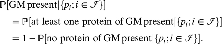The latter quantity can be expressed in terms of the conditional distribution of peptides given the proteins and of the protein priors. Further details are given in SI Gene Model Probabilities.

Independence Between the Connected Components.

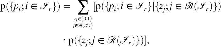
The next few sections will explain our model for protein inference, and we will thus concentrate on the bipartite graph as introduced in Fig. 1. Because the peptide probabilities or scores are considered to be realizations of random variables, we need to model their probability distribution. To do so, it is assumed that different connected components of the bipartite graph are independent. This assumption is reasonable, because we believe that peptides from the same proteins are dependent (and even more generally, peptides from the same connected component are potentially dependent), but peptides from completely different proteins which occur in different connected components are independent. The probability distribution of the peptide scores can then be modeled as

[1]

where is the set of peptides of the rth connected component of the bipartite graph.

Furthermore, the factors in the product in Eq. 1 can be rewritten as

[2]

where and there exists an edge between i and j for at least one is the range of . In other words, all the proteins having an edge to at least one of the peptides belong to .

The sum in the Eq. 2 goes over a multiindex: all the possible values for z_j (0 for absent or 1 for present in the sample) for all the proteins .

Markovian-Type Assumption.

The factors in Eq. 2 can be simplified by further assumptions. Assume that the peptides belonging to the same connected component (with r = 1,2,…,R) are independent given their matching proteins in the range . This assumption implies that dependencies among peptides are exclusively due to their common proteins. Furthermore, we make a Markovian assumption (for graphical models) which states that only the neighboring proteins matter in the conditional distribution for the peptides. The first factor in the sum of Eq. 2 can then be written as

[3]

where Ne(i) are the neighbors of the peptide i, that is, the set of all the proteins j having an edge to the peptide i.

The second factor in the Eq. 2 can be simplified by assuming that the prior occurrence of a protein is independent of the presence of other proteins:

[4]

In principle, a priori knowledge about dependencies among proteins could be implemented. Formulating such prior information is nontrivial, but it would conceptually fit into our modeling framework as well.

Probability Mixture Distribution for the Peptide Scores.

Next, a model for the probability distribution of the peptide scores given the neighboring proteins is introduced. Constructing a good model for this task is rather subjective and more data dependent than the previous modeling steps (e.g., depending whether peptide scores are probabilities or some other discriminating measure). We believe that further extensions are possible at this modeling stage to improve our protein identification approach.

We worked on peptide probabilities (or normalized scores), e.g., from PeptideProphet (17), taking values in the interval (0,1]. A mapping is used to obtain scores defined on the whole real line. The logit function is used for this task:

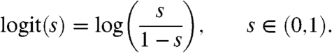Some of the peptide probabilities from the used experimental data are equal to one. This is a problem in our implementation since logit(1) is infinity. To avoid this problem, all the peptide scores are rescaled by a factor of 0.99 before the logit transform is applied. When writing p_i in the remainder of the paper, we always refer to the rescaled and logit-transformed score.

Our model assumes two different probability distributions depending on the presence of proteins (the latter is treated as an unobserved hidden variable and hence we are considering a mixture model). If none of the neighboring proteins of a peptide i are present (z_j = 0 for all j∈Ne(i)), a uniform distribution with the density function f₀(·) is assumed. A piecewise linear density f₁(·) is assumed if at least one of the neighboring proteins is present.

Hence, the mixture model is

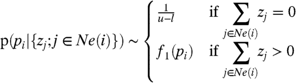[5]

with

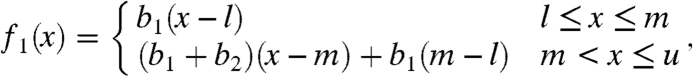[6]

where b₁ > 0, b₂≥0 are unknown parameters and 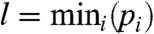, m = median_i(p_i), and . The density function f₁(x) must fulfill

[7]

One of the parameters b₁ or b₂ has to be estimated. The second one can then be computed with the constraint on the integral.

The form of the densities f₀(·) and f₁(·) were chosen empirically based on the logit-transformed PeptideProphet scores. For other scores, these functions may have to be adapted.

At this point, the model for the probability distribution of the peptide scores can be summarized by the following equation:

[8]

where p(p_i|{z_j; j∈Ne(i)}) is defined in Eq. 5.

Shared Peptides.

A shared peptide matches to two or more proteins. Shared peptides occur most of the time because of homologous proteins, splice variants, or redundant entries in the protein sequence database (16). As a consequence of our modeling assumptions, shared peptides contribute to increase or decrease (relative to single peptides) the probability for presence of a protein, depending on whether the peptide scores are above or below the median of all peptide scores. A conceptual example is given in SI Shared Peptides.

Summary of the Assumptions.

The main assumptions in our model are as follows:

1. The peptide probabilities or scores are modeled as random quantities. This allows one to account for statistical uncertainty and variability.

2. The connected components of the bipartite graph for proteins and peptides induce independence between peptide scores from different connected components. However, peptides within the same connected component can be strongly dependent.

3. Peptide scores are independent given their neighboring proteins. This is a Markovian assumption (on graphical models) which encompasses a broad class of interesting dependence structures [see, for example, Lauritzen (19)].

4. The prior probability that a protein is present or not in the sample is independent of the presence of the other proteins. This simplifies the specification of a prior distribution: Extensions to more general prior distributions are conceptually straightforward but the computation for fitting the model becomes more expensive.

   However, this does not mean that proteins are independent. In the model, the dependence among proteins within the same connected component is still present. We only assume independent priors as starting values to make the computations easier.

5. The model for peptide scores is a mixture model. As such, it belongs to a popular class of statistical models for inferring presence or absence of an unobserved hidden variable (i.e., a protein in our context).

Maximum Likelihood Estimation and Computation.

One of the parameters b₁, b₂ in Eq. 6 has to be estimated from the data of the current sample of interest. We use maximum likelihood estimation for this task. More details can be found in SI Log-Likelihood.

Ideally, the prior probabilities p(z_j) (see formula 8) are related to some biological information and there would be a specific value p(z_j) for each protein j. Because this biological knowledge is often missing, we simplify to the point where it is assumed that all the proteins have the same prior probability of being in the sample, i.e., p(z_j) ≡ π for all j. Such a parameter π can then be estimated from the data. Using such an approach, the parameter π is not a prior probability from a Bayesian statistics framework anymore. More details can be found in SI Log-Likelihood.

Computation of the Protein Probabilities

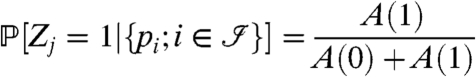
Formulas 1 and 8 describe how to calculate the distribution of the peptide scores. The goal here is to compute the probability that a protein j is present given the peptide scores:

[9]

with

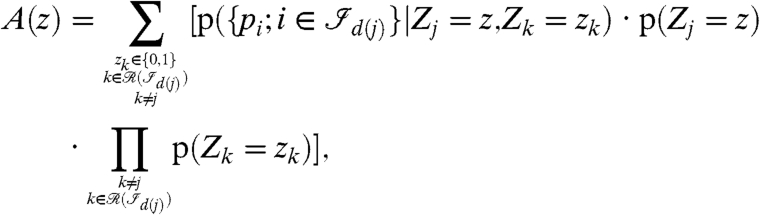[10]

where d(j) is the index of the connected component holding the protein j. A derivation of formula 10 and more details about the computations for A(z) are given in SI Protein Probabilities.

The value of in Eq. 9 involves the estimated parameters , and the protein priors.

The computational effort for large connected components is considerable and needs a workaround. Details are given in SI Sampling for Large Connected Components.

Validation of the Model

We compared our results to the protein scores computed by ProteinProphet (5) and MSBayesPro (12) to evaluate MIPGEM. To be able to compare our results to the output from other methods, there are two issues to be addressed. The first one concerns the accounting of contaminants, whereas the second one is specific to ProteinProphet.

Maximize Data Quality Prior to Protein Inference.

In particular for large real-world datasets, it is important to assess how many false positive identifications are observed.

Because the peptide-spectrum matching process will only produce true positive assignments if the corresponding protein is present in the database, contaminants that can get added to the protein mixture during the experimental handling such as human keratins and others, should ideally be added to the database. Due to their abundance, they otherwise could lead to false positive peptide and protein identifications (20).

This has an important consequence for the interpretation of the results. Identified contaminants could be counted as true positives. On the other hand, a missed contaminant should definitely not be counted as a false negative. Hence, there is a risk of getting true positives for “free” while not counting the eventual false negatives. To achieve a more objective accounting, we decided not to consider the contaminants, neither in our model nor in the reference methods.

The same sets of true proteins and contaminants were used to interpret the results from all methods. For the two synthetic mixtures, lists with the corresponding proteins are given in SI Additional Information About the Datasets.

ProteinProphet.

The output from ProteinProphet (5) is structured in groups. Each group gets a probability that at least one of the proteins in the group is present in the sample. Furthermore, a probability for each distinguishable protein is computed. For ambiguous proteins, the computed number corresponds to the probability of seeing at least one of these ambiguous proteins. If the sequences of all ambiguous protein accessions are identical, we consider the sequence as unambiguously identified.

From ProteinProphet’s output we consider all unambiguously identified proteins. We make sure to only keep sequences having at least one contributing peptide (after the reallocation of peptides performed by this method). When drawing the ROC (receiver operating characteristic) curves about true and false positive findings, we consider two scenarios: (i) take all these sequences and consider the protein probabilities (labeled with “ProteinProphet—prot prob”) and (ii) discard proteins belonging to a group and use group probabilities for groups identifying a single protein sequence (labeled with “ProteinProphet—group prob”). The differences in the plots between these two interpretations are very small.

Because of ProteinProphet’s nature to group proteins that cannot be distinguished based on the experimental peptide evidence, we can only take into consideration unambiguously identified proteins when comparing our results to the output of the two reference methods. However, note that in MIPGEM each protein sequence gets its own score. Each protein sequence appears only once in our graph, even if it corresponds to several accession numbers. We do no further grouping of ambiguous sequences, but compute a probability for each of them. Ambiguous proteins then get the same score. This score automatically decreases with the number of ambiguous proteins (for the same set of peptides). This is a major difference to ProteinProphet where ambiguous proteins are simply “put” together, and the user only gets a probability of at least one of these proteins being in the sample. We think that it is much better to report the probabilities for each separate protein instead of such a group probability, which may lead to misinterpretations of the results.

MSBayesPro.

The rules for a protein to be considered as identified in MSBayesPro (12) are discussed in SI Comparison with Other Protein Inference Models.

General Remarks.

We consider, in general, distinct peptides, even if identified by several mass spectra similarly to ref. 7. If the peptide sequences are the same, but the charge states differ, we consider a separate instance of the peptide for each of the detected charge states. Only peptides with a PeptideProphet score larger than 0.9 are used for the protein inference. The sensitivity of MIPGEM’s output with respect to the chosen cutoff for the peptide scores is discussed in SI Additional Figures and Tables.

The two synthetic samples, the mixture of 18 proteins (21) and Sigma49 (9, 22), are “toy” datasets of low protein complexity. It is commonly agreed that showing a good performance on these samples is nice, but does not say much about the method’s ability to handle real datasets. We therefore chose three further complex protein datasets that have recently been described in the literature for testing (13, 23, 24).

Mixture of 18 Purified Proteins.

The results are shown in Fig. 3A. Details about the dataset are given in SI Mixture of 18 Purified Proteins.

Fig. 3.

Number of true positives (#TP) versus number of false positives (#FP) for the mixture of 18 purified proteins (A), for the Sigma49 (B) and for the S. cerevisiae (C) datasets.

The number of true positives (TPs) and false positives (FPs) was computed as described before. The differences between the results of the three methods are small: MIPGEM performs slightly worse.

Sigma49 Dataset.

The results are shown in Fig. 3B. Details about the dataset are given in SI Sigma49.

There is an important difference between our model and the two reference methods. ProteinProphet’s ROC curve goes up rapidly. It finds 22 proteins (20 TP and 2 FP) having a probability of one. MSBayesPro goes up a little less steeply by assigning a top score to 15 TPs and 2 FPs. It is not possible to run these two methods in a more conservative way. On the other hand, MIPGEM goes up straight to 13 TPs against 0 FPs, and it then flattens out. Unlike ProteinProphet and MSBayesPro, MIPGEM can be used (in principle) to achieve zero false positives.

Among our top-scoring proteins, there are also single hits (proteins identified by a single spectrum). Single hits are penalized in ProteinProphet, but not in MIPGEM. A figure showing the results of the different methods when discarding the identified single hits can be found in SI Additional Figures and Tables.

Saccharomyces cerevisiae Dataset.

The results are shown in Fig. 3C. Details about the dataset are given in SI Saccharomyces cerevisiae Dataset.

We find a similar behavior as for the Sigma49 dataset. MIPGEM exhibits zero false positives among the 320 top-scoring proteins, whereas ProteinProphet and MSBayesPro cannot produce zero false positives.

Drosophila melanogaster Dataset.

MIPGEM was also applied to complex protein samples of unknown composition. Details about the dataset are given in ref. 23 and SI Drosophila melanogaster Dataset.

Because we don’t know which proteins are present in the sample, we can only make a statement about how well the three methods agree on the identified sets of protein sequences.

ProteinProphet (5) finds 217 proteins with a probability score of one. MSBayesPro (12) detects 222 proteins with a score of one. In view of our findings for the Sigma49 dataset, we assume that these proteins also include false positives.

The intersection of proteins yielding a top score in ProteinProphet and in MSBayesPro holds 167 proteins. Unfortunately, we cannot even rank for presence of these top-scoring proteins because their probabilities, from ProteinProphet and MSBayesPro, are all equal to the maximal value of one. With MIPGEM, we can easily rank the proteins because their corresponding scores vary. The distributions of the computed protein scores are shown in SI Additional Figures and Tables. In Table 1, the n top-scoring proteins of MIPGEM are compared to (i) the set of 167 proteins in the intersection of the top-scoring proteins of both reference methods; (ii) the set of 217 proteins with a maximal score from ProteinProphet; and (iii) the set of 222 proteins with a maximal score from MSBayesPro. Each row of Table 1 displays how many proteins belong both to the reference set and to the n top-scoring proteins from MIPGEM. For this example, the overlap between the results of the three methods is perfect only up to the 25 top-scoring proteins from our model. At this stage, discrepancies appear between the results from MSBayesPro and the two other methods. The overlap between ProteinProphet and MIPGEM, however, is perfect up to the first 101 proteins. For larger numbers of identified proteins, the percentage of overlap becomes lower. The outcomes of the three approaches coincide better if the identified single hits are discarded in all models (see SI Additional Figures and Tables). Note that some of our top-scoring proteins are neither identified by ProteinProphet nor by MSBayesPro with top scores.

Table 1.

Overlap of protein identifications

n	25	50	78	101	170	200	222
Ref. set (i)	25	45	72	95	108	126	143
Ref. set (ii)	25	50	78	101	115	133	155
Ref. set (iii)	25	45	72	95	163	181	198

Arabidopsis thaliana Dataset.

In contrast to the two reference methods, our model is also designed to infer gene models. To validate this feature, we used A. thaliana pollen data where we constructed an approximate ground truth for the gene models. Details about this dataset are given in ref. 13 and SI Arabidopsis thaliana Dataset.

Fig. 4 shows the ROC curve for the identified gene models, and Fig. 2 highlights the importance of using gene model scores. ProteinProphet and MSBayesPro both lack this feature. There is no straightforward way to compare our results with their output.

Fig. 4.

Number of true positive (#TP) versus number of false positive (#FP) gene models for the A. thaliana pollen dataset. The dashed lined corresponds to the expected output from random sampling. A comparison to ProteinProphet and MSBayesPro is not possible, because these methods are not designed to infer gene model probabilities.

Discussion

MIPGEM is a rigorous statistical model for protein inference from shotgun proteomics data. It is based on a few clearly stated assumptions. In particular, we use Markovian assumptions on graphs which allow to model dependencies among and between peptides and proteins in a realistic way. In contrast to most previous solutions, we model the peptide scores as probabilistic input for the protein inference and extend our approach to also infer the probabilities at the gene model level. The latter will allow for integration with transcriptomics data even if the exact protein composition cannot be inferred. It can also be used to assess the potential of proteomics to identify different protein splice isoforms that are encoded by the same gene model (see Fig. 2D).

The model was tested on two control datasets and one “semicontrol” dataset. We found that, in comparison to ProteinProphet (5), a commonly applied software tool to summarize protein identifications based on experimental peptide evidence, MIPGEM exhibits fewer false positives among the highest ranking proteins while paying a price in terms of a larger number of false negatives. This same trend was observed compared to MSBayesPro (12), another protein inference method. Controlling the number of false positives at a low level is in accordance with statistical hypothesis testing.

Also, our approach allows for distinction on a fine level, whereas ProteinProphet and MSBayesPro often assign the maximal score of one to many proteins. In addition, in case of ambiguous proteins, we think it is much better to report probabilities for individual proteins instead of grouping these sequences as ProteinProphet does. Such protein groups with a single probability do not allow for a clear interpretation.

Our statistical modeling framework for protein and gene model inference is generic and can be extended in order to include additional parameters such as peptide detectability (25) (see, e.g., ref. 12), number of tryptic termini (10, 14), specific protein prior probabilities, or protein coverage to further improve its performance.

References

- 1.Aebersold R, Mann M. Mass spectrometry-based proteomics. Nature. 2003;422:198–207. doi: 10.1038/nature01511. [DOI] [PubMed] [Google Scholar]
- 2.Washburn MP, Wolters D, Yates JR., III Large-scale analysis of the yeast proteome by multidimensional protein identification technology. Nat Biotechnol. 2001;19:242–247. doi: 10.1038/85686. [DOI] [PubMed] [Google Scholar]
- 3.Tabb DL, McDonald WH, Yates JR., III DTASelect and contrast tools for assembling and comparing protein identifications from shotgun proteomics. J Proteome Res. 2002;1:21–26. doi: 10.1021/pr015504q. [DOI] [PMC free article] [PubMed] [Google Scholar]
- 4.Moore RE, Young MK, Lee TD. Qscore: An algorithm for evaluating sequest database search results. J Am Soc Mass Spectr. 2002;13:378–386. doi: 10.1016/S1044-0305(02)00352-5. [DOI] [PubMed] [Google Scholar]
- 5.Nesvizhskii AI, Keller A, Kolker E, Aebersold R. A statistical model for identifying proteins by tandem mass spectrometry. Anal Chem. 2003;75:4646–4658. doi: 10.1021/ac0341261. [DOI] [PubMed] [Google Scholar]
- 6.Weatherly DB, et al. A heuristic method for assigning a false-discovery rate for protein identifications from mascot database search results. Mol Cell Proteomics. 2005;4:762–772. doi: 10.1074/mcp.M400215-MCP200. [DOI] [PubMed] [Google Scholar]
- 7.Price TS, et al. EBP: Protein identification using multiple tandem mass spectrometry datasets. Mol Cell Proteomics. 2007;6:527–536. doi: 10.1074/mcp.T600049-MCP200. [DOI] [PubMed] [Google Scholar]
- 8.Feng J, Naiman DQ, Cooper B. Probability model for assessing proteins assembled from peptide sequences inferred from tandem mass spectrometry data. Anal Chem. 2007;79:3901–3911. doi: 10.1021/ac070202e. [DOI] [PubMed] [Google Scholar]
- 9.Zhang B, Chambers MC, Tabb DL. Proteomic parsimony through bipartite graph analysis improves accuracy and transparency. J Proteome Res. 2007;6:3549–3557. doi: 10.1021/pr070230d. [DOI] [PMC free article] [PubMed] [Google Scholar]
- 10.Shen C, et al. A hierarchical statistical model to assess the confidence of peptides and proteins inferred from tandem mass spectrometry. Bioinformatics. 2008;24(2):202–208. doi: 10.1093/bioinformatics/btm555. [DOI] [PubMed] [Google Scholar]
- 11.Bern M, Goldberg D. Improved ranking functions for protein and modification-site identifications. J Comput Biol. 2008;15:705–719. doi: 10.1089/cmb.2007.0119. [DOI] [PubMed] [Google Scholar]
- 12.Li YF, et al. A Bayesian approach to protein inference problem in shotgun proteomics. J Comput Biol. 2009;16(8):1183–1193. doi: 10.1089/cmb.2009.0018. [DOI] [PMC free article] [PubMed] [Google Scholar]
- 13.Grobei MA, et al. Deterministic protein inference for shotgun proteomics data provides new insights into Arabidopsis pollen development and function. Genome Res. 2009;19:1786–1800. doi: 10.1101/gr.089060.108. [DOI] [PMC free article] [PubMed] [Google Scholar]
- 14.Li Q, MacCoss M, Stephens M. A nested mixture model for protein identification using mass spectrometry. Ann Appl Statist. 2010. preprint.
- 15.Nesvizhskii AI, Vitek O, Aebersold R. Analysis and validation of proteomic data generated by tandem mass spectrometry. Nat Methods. 2007;4:787–797. doi: 10.1038/nmeth1088. [DOI] [PubMed] [Google Scholar]
- 16.Nesvizhskii AI, Aebersold R. Analysis, statistical validation and dissemination of large-scale proteomics datasets generated by tandem ms. Drug Discov Today. 2004;9:173–181. doi: 10.1016/S1359-6446(03)02978-7. [DOI] [PubMed] [Google Scholar]
- 17.Keller A, Nesvizhskii AI, Kolker E, Aebersold R. Empirical statistical model to estimate the accuracy of peptide identifications made by ms/ms and database search. Anal Chem. 2002;74:5383–5392. doi: 10.1021/ac025747h. [DOI] [PubMed] [Google Scholar]
- 18.Eng JK, McCormack AL, Yates JR., III An approach to correlate tandem mass spectral data of peptides with amino acid sequences in a protein database. J Am Soc Mass Spectr. 1994;5:976–989. doi: 10.1016/1044-0305(94)80016-2. [DOI] [PubMed] [Google Scholar]
- 19.Lauritzen SL. Graphical Models. Oxford: Oxford Science Publ; 1996. pp. 28–60. [Google Scholar]
- 20.de Godoy LMF, et al. Status of complete proteome analysis by mass spectrometry: SILAC labeled yeast as a model system. Genome Biol. 2006;7:R50. doi: 10.1186/gb-2006-7-6-r50. http://www.ncbi.nlm.nih.gov/pubmed/16784548. [DOI] [PMC free article] [PubMed] [Google Scholar]
- 21.Keller A, et al. Experimental protein mixture for validating tandem mass spectral analysis. OMICS. 2002;6:207–212. doi: 10.1089/153623102760092805. [DOI] [PubMed] [Google Scholar]
- 22.Tabb DL, Fernando CG, Chambers MC. Myrimatch: Highly accurate tandem mass spectral peptide identification by multivariate hypergeometric analysis. J Proteome Res. 2007;6:654–661. doi: 10.1021/pr0604054. [DOI] [PMC free article] [PubMed] [Google Scholar]
- 23.Brunner E, et al. A high-quality catalog of the Drosophila melanogaster proteome. Nat Biotechnol. 2007;25:576–583. doi: 10.1038/nbt1300. [DOI] [PubMed] [Google Scholar]
- 24.Ramakrishnan SR, et al. Integrating shotgun proteomics and mRNA expression data to improve protein identification. Bioinformatics. 2009;25(11):1397–403. doi: 10.1093/bioinformatics/btp168. [DOI] [PMC free article] [PubMed] [Google Scholar]
- 25.Alves P, et al. Advancement in protein inference from shotgun proteomics using peptide detectability. In Pacific Symposium on Biocomputing. 2007:409–420. http://www.ncbi.nlm.nih.gov/pubmed/17990506. [PubMed] [Google Scholar]
Associated Data
This section collects any data citations, data availability statements, or supplementary materials included in this article.