A generative model of microtubule distributions, and indirect estimation of its parameters from fluorescence microscopy images

Abstract

The microtubule network plays a critical role in many cellular processes, and quantitative models of how its organization varies across cell types and conditions are required for understanding those roles and as input to cell simulations. High-throughput image acquisition technologies are potentially valuable for this purpose, but do not provide sufficient resolution for current analysis methods that rely on tracing of individual microtubules. We describe a parametric conditional model of microtubule distribution that can generate a microtubule network in intact cells using a persistent random walk approach. The model parameters are physically meaningful as they directly describe the spatial distribution of microtubules and include the number of microtubules as well as the mean of the length distribution. We also present an indirect method for estimating the parameters of the model from three-dimensional fluorescence microscope images of cells that relies on comparing acquired images with simulated images generated from the model. Our results show that our method can reasonably recover parameters for a given query image, and we present the distributions of parameters estimated by our method for a collection of HeLa cell images.

INTRODUCTION

Understanding the many complex cellular and subcellular processes underlying biological phenomena will require approaches for obtaining spatiotemporal information for the tens of thousands of proteins expressed in a typical cell. These measurements (in many cases in the form of statistical estimates) can then be used in modeling and simulation efforts where the goal is to predict and help understand cellular systems. One such example in microtubule organization is the simulation of microtubules with motor proteins in order to understand their phenotypic behavior (1). Another example in the area of cytoskeleton organization is the simulation of actin to understand the lamellipodial behavior of a cell (2).

Among the many relevant cellular phenomena to be modeled and quantified, the subcellular spatial distribution of proteins (their location and overall organization) is important because of the crucial role that location plays in many cellular phenomena. Many neurodegenerative diseases such as Alzheimer’s and Parkinson’s are related to the malfunction of microtubule associated proteins and the microtubule network that leads to the accumulation of protein aggregates in brain cells (3). Technologies that facilitate the quantitative analysis of protein location, on a proteome-wide scale, would therefore have potentially high impact.

Many approaches have been described for obtaining subcellular location data of large numbers of protein distributions (4-8). Green fluorescent protein (GFP) tagging has emerged as the most widely used tool for this purpose and has enabled proteome-scale studies (see (9) for a prominent example using GFP-fusions in yeast). A notable exception is the work by the Human Protein Atlas project (10,11), which uses antibody-based methods and has generated millions of images for over six thousand antisera against various proteins. Although it is possible to interpret the information content in such collections visually, automated approaches can play an important role in extracting more detailed quantitative information from them (12).

Potential frameworks to characterize protein location patterns from such image data include descriptive techniques and generative models. In short, descriptive techniques seek to describe the content of images using numerical feature vectors, one vector per cell or image. These techniques enable automated subcellular location determination using supervised learning approaches (see (13), for an example) but, in the absence of any associated modeling technique, they cannot be used to provide quantitative physical information pertaining to the protein distributions. Generative models, on the other hand, generalize from examples by learning a description of the underlying process believed to give rise to the image (14). We have previously described a framework to learn generative models of multiple subcellular location patterns from cells (15). Cell membrane, nuclear and protein object models were constructed so that simulated images representing seven different subcellular location patterns could be generated. In short, one way to fully understand the location patterns of individual proteins in a given cell type is to summarize this information in the form of a model that can accurately represent the statistical variation contained in a set of fluorescence microscopy images. In the context of this work, we sought to demonstrate that physically meaningful parameters describing the process by which protein distributions are generated can also be learned from these images. We also sought to extend our previous modeling framework, which represented protein distributions as a collection of distinct objects (15), to protein distributions such as microtubule networks, that cannot be easily represented as objects.

There are several direct methods for estimation of microtubule parameters by tracing described in the current literature. For these, however, the imaging approach is either not suitable for intact cells, or the image resolution is not sufficient to discern individual microtubules throughout the entire extent of the cell (16-20). This can be seen in Figure 1 in which the high density of microtubules near the centrosomal region makes it impossible to visually or computationally extract individual tracks. Even in regions where individual tracks can be discerned (often near the boundary of the cell), tracing algorithms are invariably hindered by “crossing” tracks. One solution is to use specialized microscopy methods that greatly enhance estimation of filament like structures: Fluorescence Speckle Microscopy (21), Fluorescence Correlation Spectroscopy (22) and Stimulated Emission Depletion microscopy (23). However, these methods are not easy to apply on a proteome scale. Indirect approaches, on the other hand, are more suitable for filament structures since the structures themselves do not have to be matched exactly but rather the pattern they form in an image is matched instead. A compelling example of such an approach was used to validate models of the mitotic spindle (24). In that study, however, very limited and simple image features such as mean of fluorescence intensity was used to compare patterns in the images. Another excellent example of an indirect method was analysis of the structure and dynamics of the actin filament network in the lamellipodia of a migrating cell (25). However, images in this work were cropped to a representative region in the lamellipodia that would not be expected to yield accurate estimate parameters for the entire cell. The method of comparison used only a distribution of correlation lengths from images, which may not be adequate to completely quantify complex patterns in images resulting from overlapping filament structures.

Figure 1.

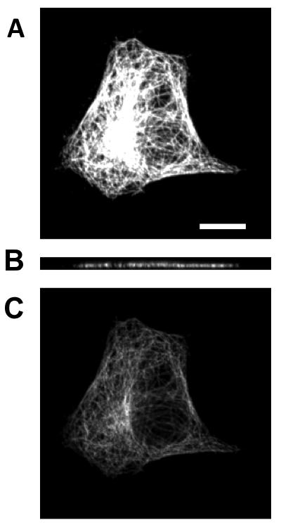
Example image from the 3D HeLa dataset. (A) shows the sum X-Y projection of the image (B) shows a slice along the X-Z and (C) shows a slice along the X-Y. The scale bar is 10 μm.

OVERVIEW OF OUR CONTRIBUTION

The principle behind the system we describe is that very basic a priori knowledge can be used to formulate models of proteins from which artificial images are generated (according to initial estimates of the parameters of the model). The model parameters are then iteratively modified until a specified similarity measure between the real input images and the artificial ones is maximized. The critical steps in this procedure are shown in Figure 2 and include microtubule pattern generation, image simulation, and comparison with a real microscopic image. These steps are assembled into an optimization procedure to be detailed below. We have obtained preliminary results with both simulated and real data showing that extraction of such parameters for microtubule distributions is feasible.

Figure 2.

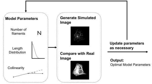
Overview of the Approach

MATERIALS AND METHODS

DATA ACQUISITION

Images of 3D HeLa cells previously obtained by three-color confocal immunofluorescence microscopy (26) were used. This collection contains approximately 50 images for each of nine different proteins, including tubulin. Each image consists of three channels, one reflecting the distribution of DNA (as visualized with propidium iodide after RNAse digestion), total protein (as visualized with a non-specific reactive probe), and a specific protein (as visualized with a well-characterized monoclonal antibody). The spacing between voxels in the image is 0.05 microns in the focal plane (the X and Y directions) and 0.2 microns in the axial dimension (the Z direction).

COMPUTATIONAL METHODS

Preprocessing

The raw images were first downsampled in the X-Y dimension due to memory and computational issues from 0.05 microns to 0.2 microns per voxel. Hence the final voxel spacing is uniform in all three directions; the number of voxels in the X or Y dimension reduced from 1024 to 256.

Estimation of the point spread functions (PSF)

Three point spread functions were estimated for the cell membrane, nuclear membrane and alpha-tubulin-GFP channels. The point spread functions for the cell membrane and nuclear channels were estimated using the Diffraction PSF 3D ImageJ plugin (http://www.optinav.com/Diffraction-PSF-3D.htm). The plugin outputs the emission point spread function. The confocal point spread function is approximated as the square of the emission point spread function. The point spread function for alpha-tubulin-GFP channel was directly estimated from the fluorescence microscopy image. Line intensities along the X dimension and along the Z dimension were computed with clearly distinguishable and well separated microtubules wrapped around the nucleus. The line profiles were registered and truncated to size 7, and averaged for the X and Z dimension. A 3D Gaussian was manually fit and was used as the point spread function.

Segmentation to estimate the cytosolic space

Each channel of each image was corrected for background fluorescence by subtraction of the most common pixel value and deconvolved with a theoretical point spread function for the nuclear channel and the cell membrane channel. The images were segmented into single cell regions using seeded watershed segmentation. The cell boundary and nuclear boundary in each slice was then found using the active contour method on the deconvolved cell membrane channel and nucleus channel respectively (27).

Estimating Location of the centrosome

The tubulin image was convolved with a 3×3×3 averaging filter. The location of the centrosome was estimated to be the voxel with the maximum intensity.

Growth Model of Microtubule Patterns

The model of microtubule distribution was constructed using a growth model conditioned on the centrosome location, cytosolic space and the parameters of the model. The growth model consists of generating microtubules as points on a star network with the hub as the centrosome. Let X₀ denote the location, in three dimensions, of the center of the centrosome of a given cell. Assuming the centrosome a sphere, we fix the diameter of a centrosomal structure to be approximately 0.4 μm. We generate N random points $X_0^i:i\in Z,1\le i\le N$ inside the volume of the sphere where N is the number of microtubules to be generated. Each point in the sphere is extended in a random direction to a new point $X_1^i$ with steplength γ. These short segments are further extended by picking a point $X_2^i$ with step length γ that satisfies two constraints. The stiffness constraint is as follows:

$$\cos \alpha \le v_1•v_2\le 1$$ (1)

$$\begin{array}{cc}\hfill \hfill & \hfill v_1=\frac{X_1-X_0}{\Vert X_1-X_0\Vert }\hfill \\ \hfill \text{with}\hfill & \hfill \hfill \\ \hfill \hfill & \hfill v_2=\frac{X_2-X_1}{\Vert X_2-X_1\Vert }\hfill \end{array}$$ (2)

and α – angle between (X₂ – X₁) and (X₁ – X₀) . In our model, cos(α) is called the collinearity parameter. Points are also constrained to be generated in the cytosolic space using a lookup image that was estimated using segmentation.

We model the length distribution as a truncated normal distribution (28). The normal distribution is truncated such that there can be no negative lengths. This distribution was shown earlier to fit the lengths of microtubules well in the meiotic spindle (29). The random variable X ~ N(μ,σ²) conditioned on (0 < X < ∞) follows a probability density function:

$$f(x;\mu ,\sigma ,a,b)=\frac{\frac{1}{\sigma }\varphi \left(\frac{x-\mu }{\sigma }\right)}{1-\Phi \left(\frac{-\mu }{\sigma }\right)}$$ (3)

where ϕ is the probability density function of the standard normal distribution and Φ is the cumulative distribution function. This distribution is sampled N times, where N is the number of microtubules. The microtubule elongation procedure is iterated for each of N microtubules, until the sampled lengths of the microtubule polymer is satisfied. The following are thus the model parameters:

1. Diameter of the centrosomal sphere: 0.4 μm (fixed)

2. step length: 0.2 μm (fixed)

3. number of microtubules: n

4. collinearity: cos α

5. mean of the normal distribution: μ

6. standard deviation of the normal distribution: σ

Simulated Pattern to Simulated Image

The microtubule structure model is convolved with the estimated point spread function to simulate a fluorescence microscopy image generation process. The resulting polymerized tubulin image is multiplied by a scalar such that the single microtubule peak intensity from the simulated image matches the mean of the peak single microtubule intensity in the raw image.

Grid Generation

We generated a grid of simulated images by varying model parameters. The range of the values for the standard deviation of the length distribution and the collinearity (cos α) did not take all possible values, but was based on how much real variation we believe is present. The parameters varied took the following values:

• n = 5, 25, 50, 75, 100, 125, 150, 175, 200, 225, 250, 275, 300

• μ = 5, 25, 50, 75, 100, 125, 150 microns

• σ = 1, 5, 10, 15, 20, 25 microns

• cos α = 0.9, 0.95, 0.98

Thus, for a given cell morphology, a total of 1638 images were generated.

Feature Computation

(1) Thirteen 3D Haralick texture features were computed from a single co-occurrence matrix for all the 13 directions for each image was calculated (30). Two more sets of these features were computed by downsampling the image by two and by four. (2) The image was discretized in subvolumes radially starting from the centrosome. Radial intensity features were calculated by computing the total intensity in these subvolumes and normalizing by their respective volumes. (3) Histogram features were computed that consist of standard measures such as Mean, Variance, Skewness, Kurtosis, Energy and Entropy. (4) The total intensity was computed as a feature that is the sum total of all graylevels values in the 3D image.

Distance Function and Matching

A diagonal matrix D was computed that contain the variances of the features. This variance matrix was then used to compute the Normalized Euclidean distance between a feature vector x_s computed from a set of simulated microtubules (simulated image) and a feature vector x_r corresponding to the image based on which the microtubule simulation was computed (raw image). In this case, the Normalized Euclidean distance is given by

$$d_{rs}^2=(x_r-x_s)D^{-1}{(x_r-x_s)}^{\prime }$$

For any query image, we computed the Normalized Euclidean distances from each of the large grid of simulated images. The optimization problem estimates parameters by minimizing the Normalized Euclidean distance: $[n,\mu ,\sigma ,\cos \alpha ]=\mathrm{argmin}{d}_{rs}^2$.

Sensitivity Analysis

To determine how well model parameters can be recovered by matching, 400 parameter sets were randomly selected from the grid. Images were generated based on these parameter sets with different random number generator seeds than those from the images in the image grid. Image matching was done with each of the 400 query images.

The error metric used was the mean absolute percentage error (MAPE).

$$\mathit{MAPE}=\frac{1}{400}\sum _{t=1}^{400}\mid \frac{R_t-S_t}{R_t}\mid$$

where

• R_t - Query Image parameters

• S_t - Estimated Image parameters

RESULTS

GENERATIVE MODEL OF MICROTUBULE PATTERNS

Cell and nuclear boundaries and Centrosome location

Typically, microtubules grow out from the centrosome and grow within the cytosolic space of the cell. Hence, a generative model of the microtubule pattern must be conditioned (dependent) on a nuclear model and a cell membrane model. In order to build a model from a 3D cell image, the nuclear and cell membrane channels were deconvolved with their respective point spread functions and segmented semi-automatically using the Active Contour without Edges approach (see Methods). The central point from which microtubules grow is the centrosome, and its position can be directly estimated from the tubulin channel. Figure 3 shows the cell boundary, the nucleus boundary and the centrosome location for a slice of the image in Figure 1.

Figure 3.

Cell and Nuclear boundaries and Centrosome Location

Microtubule Growth Model and Image Simulation

The growth model consists of generating different numbers of microtubules (each with a specified length) by extending short segments starting from a single point in the cytosolic space (the centrosome). The model parameters that are varied are the number of microtubules, the mean and standard deviation of the length distribution of microtubules, and the collinearity (see Methods). Given specific values for each parameter, an image can be generated that simulates a microtubule distribution, as it would be imaged under the specified condition. Figure 4 shows a model of the microtubule network generated by this method and an image that results from convolving it with a point spread function.

Figure 4.

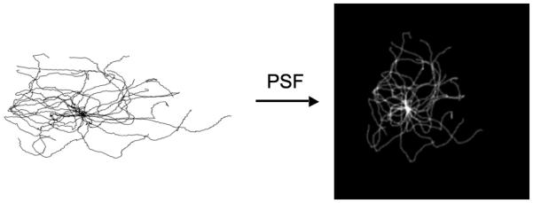
An example rendering of a microtubule 3D model (view from a 3D corner) converted to image (sum projected along Z-axis) using a point spread function. The background color is changed to reflect model and image.

ESTIMATING MODEL PARAMETERS

A grid of simulated images was generated using the model by varying the model parameters. Image features, numerical descriptors that encode the image content, were then calculated for both real and simulated images (see Methods). We measured the similarity between the query image and each of the simulated images by computing the Normalized Euclidean distance in feature space. The best fit parameters were chosen as the ones minimizing the Normalized Euclidean distance.

EVALUATING THE MATCHING PROCEDURE USING SIMULATED DATA

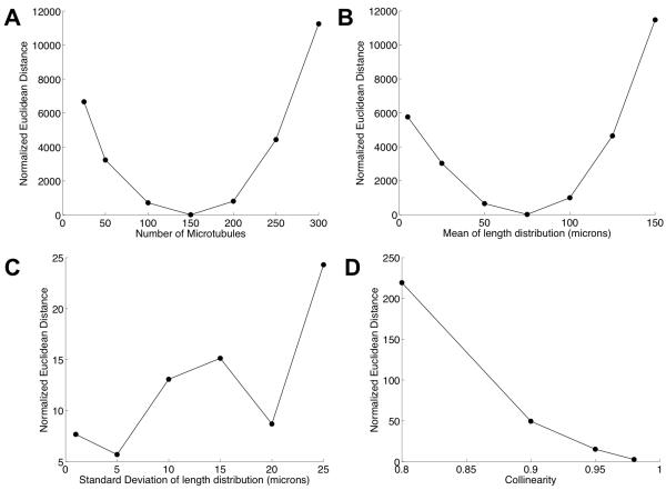
In order to check the model’s ability to recover parameters when these are known, images of microtubule patterns were simulated using the methodology described. For each simulation we tested whether the estimation procedure could be used to recover the known parameter values. The cost function is dependent on the choice of features computed from the images and the distance metric in feature space. A plot of the Normalized Euclidean distance as a function of different parameters around the vicinity of the optimal parameters (Number of microtubules = 150, Mean of length distribution = 75 microns, Standard Devation of length distribution = 10 microns, Collinearity = 0.95) is shown in Figure 5. The cost functions for the parameters show clear minima for the number of microtubules and the mean of the length distribution of microtubules, suggesting that the method of minimization could potentially recover parameters. However, in order to test this, we computed the accuracy of the method on simulated data. Table 1 shows the average over four realizations of the mean absolute percent error (MAPE) as a measure of the accuracy of recovering model parameters (See Methods). Various feature sets were tested in various combinations, and the error was observed to be minimum when all the six sets of features were used in the distance function. All the subsequent analyses were performed using all six feature sets in the distance function. Since, the growth model is stochastic, we also studied the error as a function of number of average realizations (computing a distance between a query feature vector and an average feature vector over the number of realizations for each parameter set). The error was only observed to decrease by at most a few percentage points (e.g., from an error of 8.7% to 7% for the number of microtubules) as we increased the number of realizations (data not shown). Hence, in order to reduce computation costs, all subsequent comparisons of query images with synthetic images were performed for only a single realization of the parameter set.

Figure 5.

Cost Function Plots for (A) Number of Microtubules (B) The Mean and Standard Deviation (C) of the length distribution of microtubules and (D) Collinearity

TABLE 1.

Error estimates for parameter recovery

FEATURE SETS	MEAN ABSOLUTE PERCENT ERROR (AVERAGE OVER FOUR REALIZATIONS)
	Number of Microtubules	Mean of length distribution of Microtubules (μm)	Standard deviation of length distribution of microtubules (μm)	Collinearity	Total
tot	70	102	141	3.9	316.9
his	12	17	221	2.5	252.5
har	10	19	226	1.5	256.5
ha2	14	24	230	1.7	269.7
ha4	17	32	233	1.7	283.7
rad	30	53	235	1.7	319.7
har, rad	10	19	233	1.2	263.2
tot, har	10	18	223	1.5	252.5
tot, rad	27	48	232	1.5	308.5
his, har	8	15	231	1.3	255.3
har, ha2, ha4	12	21	223	1.5	257.5
tot, har, ha2, ha4	12	21	222	1.4	256.5
har, ha2, ha4, rad	12	21	235	1.3	269.3
his, har, ha2, ha4, rad	9	15	227	1.2	252.2
tot, his, har, ha2, ha4, rad	9	15	226	1.2	251.2

• rad – Radial Intensity Features
• his – Histogram features
• har – Haralick Texture features
• ha2 - Haralick Texture features downsampled by 2
• ha4 - Haralick Texture features downsampled by 4
• tot – Total Intensity Feature

ESTIMATING PARAMETERS FROM A 3D HeLa IMAGE DATASET

Using this approach, we next estimated parameters from the images in the 3D HeLa dataset. In these computations we restricted the search to be conducted over parameter values that produced images of similar total tubulin as the input real image. This was done by first estimating the amount of variation in the peak intensity of a single microtubule. We chose one standard deviation of this variation and converted it into a standard deviation of total tubulin using the following formula:

$${\text{Total Tubulin}}_{\lim }=\frac{\left(\sum _{\text{pixels}}\text{image}\right)I_{\text{mean}}}{\gamma I_{\lim }}$$

where:

• I_mean is the mean of peak single microtubule intensity estimated

• I_lim is the upper or lower limit of intensity that is one standard deviation away from I_mean

• γ is the total intensity from a simulated microtubule point

• The simulated images in the grid were searched over this band of total tubulin.

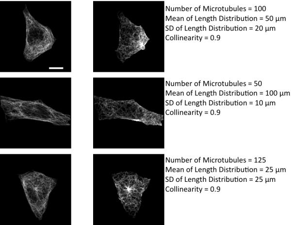
For the 3D image shown in Figure 1, the optimal parameters are: number of microtubules = 175; mean of the length distribution = 25 microns; standard deviation of the length distribution = 15 microns and the collinearity = 0.9. The simulated image corresponding to the optimal parameter set based on the matching is shown in the center column of Figure 6. In order to check if a visually reasonable match was picked by the algorithm, variations across the best match are also shown with images of varying number of microtubules (A), mean of the length distribution (B), standard deviation of the length distribution (C), and the collinearity of the microtubules (D). The leftmost image of Figure 6A shows an example of a bad parameter set that has very few microtubules. Figure 7 shows the estimated images and parameters for three cells in the 3D HeLa dataset. We also present the estimated parameters for 42 images from the dataset as histograms for each of the parameters (Figure 8).

Figure 6.

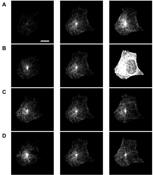
Effect of variation of model parameters on image appearance. The image whose parameters provide the best match to the image in Figure 1 is shown in the center column, and images with lower or higher values of each parameter are shown in the left and right columns, respectively. (A) Number of Microtubules (B) The Mean and Standard Deviation (C) of the length distribution of microtubules and (D) Collinearity. The scale bar is 10 μm.

Figure 7.

Query images (left column) from the 3D HeLa dataset and Estimated Images (right column) along with the estimated model parameters. The scale bar is 10 μm.

Figure 8.

Histograms of the parameters estimated for 42 cells of the 3D HeLa dataset. (A) Number of Microtubules (B) The Mean and Standard Deviation (C) of the length distribution of microtubules and (D) Collinearity

DISCUSSION

We presented a model-based approach to generate microtubule patterns that mimic some of the aspects of microtubule distributions in live cells. The algorithm generates images and measures similarity between each of the generated images and the query image by computing a Normalized Euclidean distance in feature space. The structural information about the microtubule distribution in a query image is approximated as the parameters of the generative model that generated the simulated image with the smallest Normalized Euclidean distance.

We have used a stochastic path generation algorithm to create microtubule distributions. The microtubule segments in our growth model are extended using a persistent random walk procedure where successive segments are related by a range of correlation coefficients (31). The collinearity parameter used here is a lower bound on the correlation coefficient (with the upper bound fixed at one) that can be understood as a single stiffness parameter. A related stiffness parameter that is commonly used in persistent random walk methods is the persistence length that can also be estimated from our growth model. The persistent random walk growth model is simple approach but has been used previously to generate microtubule filament patterns (32).

We have validated our parameter estimation approach using simulated data. Using the same modeling for simulation and recovery, results showed that the average error for recovering the number of microtubules in an image was about 9% while the error in the recovery of the mean length parameter was around 15%. We have also extracted microtubule distribution parameters from real images. In this case results are harder to interpret since the correct values are unknown. Overall, the recovered parameters are able to generate images of similar overall appearance to those of the corresponding real images. Also, the ranges of recovered parameter values (Figure 8) are of the appropriate order according to the findings in a study of microtubules in intact cells (33).

FUTURE DIRECTION

Although we have validated our methods using simulated data, and have used them to estimate parameters that appear to be reasonable from real data, we believe more can be done to further increase our confidence in these estimates. One of our future plans along this direction is to estimate parameters from cells under conditions where we expect the number and length of microtubules to change (such as in the presence of microtubule depolymerizing drugs like nocodazole). We plan to test whether the estimated parameters follow the expected behavior, and if not, to modify the model or the estimation approach appropriately.

In addition, although our modeling approach at this point is relatively simple, it can be easily expanded to incorporate more biologically relevant information. For example, our growth model can be made to include kinetic parameters such as growth and shrinkage rates to model dynamic instability of microtubules, or parameters that capture its interaction with molecular motors (34). It may be possible to incorporate some of these parameters by mapping them to the current model parameters (such as length distribution).

In the future, we anticipate that our model can be merged with generative models of other protein patterns. Microtubules are critical for intracellular transport and vesicles that are transported by molecular motors along microtubules. There are numerous other protein pattern images of microtubule associated proteins (MAPs) such as the microtubule end binding protein (mEB1), that are dependent on microtubule network. The model will be able to generate instances of protein patterns that are dependent on the microtubules (such as lysosomal proteins and microtubule end binding proteins).

The current approach can be used to learn models for other structures that have network/filamentous appearance. Particularly, patterns that make up the cell cytoskeleton such as actin and intermediate filaments, or proteins that make up the connective tissue such as collagen fibers, may be quantified by this method.

REFERENCES

- 1.Nedelec F. Computer simulations reveal motor properties generating stable antiparallel microtubule interactions. J Cell Biol. 2002;158(6):1005–15. doi: 10.1083/jcb.200202051. [DOI] [PMC free article] [PubMed] [Google Scholar]
- 2.Schaus TE, Taylor EW, Borisy GG. Self-organization of actin filament orientation in the dendritic-nucleation/array-treadmilling model. Proc Natl Acad Sci U S A. 2007;104(17):7086–91. doi: 10.1073/pnas.0701943104. [DOI] [PMC free article] [PubMed] [Google Scholar]
- 3.Richter-Landsberg C. The cytoskeleton in oligodendrocytes. Microtubule dynamics in health and disease. J Mol Neurosci. 2008;35(1):55–63. doi: 10.1007/s12031-007-9017-7. [DOI] [PubMed] [Google Scholar]
- 4.Hoja MR, Wahlestedt C, Hoog C. A visual intracellular classification strategy for uncharacterized human proteins. Exp Cell Res. 2000;259(1):239–46. doi: 10.1006/excr.2000.4948. [DOI] [PubMed] [Google Scholar]
- 5.Jarvik JW, Fisher GW, Shi C, Hennen L, Hauser C, Adler S, Berget PB. In vivo functional proteomics: mammalian genome annotation using CD-tagging. Biotechniques. 2002;33(4):852–4. 856, 858–60. doi: 10.2144/02334rr02. passim. [DOI] [PubMed] [Google Scholar]
- 6.Koroleva OA, Tomlinson ML, Leader D, Shaw P, Doonan JH. High-throughput protein localization in Arabidopsis using Agrobacterium-mediated transient expression of GFP-ORF fusions. Plant J. 2005;41(1):162–74. doi: 10.1111/j.1365-313X.2004.02281.x. [DOI] [PubMed] [Google Scholar]
- 7.Kumar A, Agarwal S, Heyman JA, Matson S, Heidtman M, Piccirillo S, Umansky L, Drawid A, Jansen R, Liu Y. Subcellular localization of the yeast proteome. Genes Dev. 2002;16(6):707–19. doi: 10.1101/gad.970902. others. [DOI] [PMC free article] [PubMed] [Google Scholar]
- 8.Ross-Macdonald P, Coelho PS, Roemer T, Agarwal S, Kumar A, Jansen R, Cheung KH, Sheehan A, Symoniatis D, Umansky L. Large-scale analysis of the yeast genome by transposon tagging and gene disruption. Nature. 1999;402(6760):413–8. doi: 10.1038/46558. others. [DOI] [PubMed] [Google Scholar]
- 9.Huh WK, Falvo JV, Gerke LC, Carroll AS, Howson RW, Weissman JS, O’Shea EK. Global analysis of protein localization in budding yeast. Nature. 2003;425(6959):686–91. doi: 10.1038/nature02026. [DOI] [PubMed] [Google Scholar]
- 10.Barbe L, Lundberg E, Oksvold P, Stenius A, Lewin E, Bjorling E, Asplund A, Ponten F, Brismar H, Uhlen M. Toward a confocal subcellular atlas of the human proteome. Mol Cell Proteomics. 2008;7(3):499–508. doi: 10.1074/mcp.M700325-MCP200. others. [DOI] [PubMed] [Google Scholar]
- 11.Uhlen M, Bjorling E, Agaton C, Szigyarto CA, Amini B, Andersen E, Andersson AC, Angelidou P, Asplund A, Asplund C. A human protein atlas for normal and cancer tissues based on antibody proteomics. Mol Cell Proteomics. 2005;4(12):1920–32. doi: 10.1074/mcp.M500279-MCP200. others. [DOI] [PubMed] [Google Scholar]
- 12.Glory E, Murphy RF. Automated subcellular location determination and high-throughput microscopy. Dev Cell. 2007;12(1):7–16. doi: 10.1016/j.devcel.2006.12.007. [DOI] [PubMed] [Google Scholar]
- 13.Boland MV, Murphy RF. A neural network classifier capable of recognizing the patterns of all major subcellular structures in fluorescence microscope images of HeLa cells. Bioinformatics. 2001;17(12):1213–23. doi: 10.1093/bioinformatics/17.12.1213. [DOI] [PubMed] [Google Scholar]
- 14.Murphy RF. Systematic Description Of Subcellular Location For Integration With Proteomics Databases And Systems Biology Modeling. 2007. pp. 1052–1055.
- 15.Zhao T, Murphy RF. Automated learning of generative models for subcellular location: building blocks for systems biology. Cytometry A. 2007;71(12):978–90. doi: 10.1002/cyto.a.20487. [DOI] [PubMed] [Google Scholar]
- 16.Jiang M, Ji Q, McEwen B. Model-based automated segmentation of kinetochore microtubule from electron tomography. Conf Proc IEEE Eng Med Biol Soc. 2004;3:1656–9. doi: 10.1109/IEMBS.2004.1403500. [DOI] [PubMed] [Google Scholar]
- 17.Lebbink MN, Geerts WJ, van der Krift TP, Bouwhuis M, Hertzberger LO, Verkleij AJ, Koster AJ. Template matching as a tool for annotation of tomograms of stained biological structures. J Struct Biol. 2007;158(3):327–35. doi: 10.1016/j.jsb.2006.12.001. [DOI] [PubMed] [Google Scholar]
- 18.Lichen L, Qiang J, McEwen BF. Extraction of 3D microtubules axes from cellular electron tomography images. 2002. pp. 804–807.
- 19.Santamaría-Pang A, Bîldea TS, Colbert CM, Saggau P, Kakadiaris IA. Towards segmentation of irregular tubular structures in 3D confocal microscope images. Copenhangen, Denmark: 2006. pp. 78–85. [Google Scholar]
- 20.Sargin ME, Altinok A, Kiris E, Feinstein SC, Wilson L, Rose K, Manjunath BS. Tracing Microtubules in Live Cell Images. 2007. pp. 296–299. [DOI] [PMC free article] [PubMed]
- 21.Ponti A, Matov A, Adams M, Gupton S, Waterman-Storer CM, Danuser G. Periodic patterns of actin turnover in lamellipodia and lamellae of migrating epithelial cells analyzed by quantitative Fluorescent Speckle Microscopy. Biophys J. 2005;89(5):3456–69. doi: 10.1529/biophysj.104.058701. [DOI] [PMC free article] [PubMed] [Google Scholar]
- 22.Sisan DR, Arevalo R, Graves C, McAllister R, Urbach JS. Spatially resolved fluorescence correlation spectroscopy using a spinning disk confocal microscope. Biophys J. 2006;91(11):4241–52. doi: 10.1529/biophysj.106.084251. [DOI] [PMC free article] [PubMed] [Google Scholar]
- 23.Donnert G, Keller J, Medda R, Andrei MA, Rizzoli SO, Luhrmann R, Jahn R, Eggeling C, Hell SW. Macromolecular-scale resolution in biological fluorescence microscopy. Proc Natl Acad Sci U S A. 2006;103(31):11440–5. doi: 10.1073/pnas.0604965103. [DOI] [PMC free article] [PubMed] [Google Scholar]
- 24.Sprague BL, Pearson CG, Maddox PS, Bloom KS, Salmon ED, Odde DJ. Mechanisms of microtubule-based kinetochore positioning in the yeast metaphase spindle. Biophys J. 2003;84(6):3529–46. doi: 10.1016/S0006-3495(03)75087-5. [DOI] [PMC free article] [PubMed] [Google Scholar]
- 25.Schaub S, Meister JJ, Verkhovsky AB. Analysis of actin filament network organization in lamellipodia by comparing experimental and simulated images. J Cell Sci. 2007;120(Pt 8):1491–500. doi: 10.1242/jcs.03379. [DOI] [PubMed] [Google Scholar]
- 26.Velliste M, Murphy RF. Automated determination of protein subcellular locations from 3D fluorescence microscope images. 2002. pp. 867–870.
- 27.Chan TF, Vese LA. Active contours without edges. IEEE Trans Image Process. 2001;10(2):266–77. doi: 10.1109/83.902291. [DOI] [PubMed] [Google Scholar]
- 28.Johnson NL, Kotz S. Continuous univariate distributions. 2 v. Hougton Mifflin; New York: 1970. [Google Scholar]
- 29.Yang G, Houghtaling BR, Gaetz J, Liu JZ, Danuser G, Kapoor TM. Architectural dynamics of the meiotic spindle revealed by single-fluorophore imaging. Nat Cell Biol. 2007;9(11):1233–42. doi: 10.1038/ncb1643. [DOI] [PubMed] [Google Scholar]
- 30.Chen X, Velliste M, Weinstein S, Jarvik JW, Murphy RF. Location proteomics-Building subcellular location trees from high resolution 3D fluorescence microscope images of randomly-tagged proteins. 2003. pp. 298–306.
- 31.Rudnick JA, Gaspari GD. Elements of the random walk : an introduction for advanced students and researchers. Cambridge University Press; Cambridge ; New York: 2004. p. xv.p. 329. [Google Scholar]
- 32.Brangwynne CP, MacKintosh FC, Weitz DA. Force fluctuations and polymerization dynamics of intracellular microtubules. Proc Natl Acad Sci U S A. 2007;104(41):16128–33. doi: 10.1073/pnas.0703094104. [DOI] [PMC free article] [PubMed] [Google Scholar]
- 33.Gorbsky G, Borisy GG. Microtubule distribution in cultured cells and intact tissues: improved immunolabeling resolution through the use of reversible embedment cytochemistry. Proc Natl Acad Sci U S A. 1985;82(20):6889–93. doi: 10.1073/pnas.82.20.6889. [DOI] [PMC free article] [PubMed] [Google Scholar]
- 34.Karsenti E, Nedelec F, Surrey T. Modelling microtubule patterns. Nat Cell Biol. 2006;8(11):1204–11. doi: 10.1038/ncb1498. [DOI] [PubMed] [Google Scholar]