Automated Interpretation of Subcellular Patterns in Fluorescence Microscope Images for Location Proteomics

Abstract

Proteomics, the large scale identification and characterization of many or all proteins expressed in a given cell type, has become a major area of biological research. In addition to information on protein sequence, structure and expression levels, knowledge of a protein’s subcellular location is essential to a complete understanding of its functions. Currently subcellular location patterns are routinely determined by visual inspection of fluorescence microscope images. We review here research aimed at creating systems for automated, systematic determination of location. These employ numerical feature extraction from images, feature reduction to identify the most useful features, and various supervised learning (classification) and unsupervised learning (clustering) methods. These methods have been shown to perform significantly better than human interpretation of the same images. When coupled with technologies for tagging large numbers of proteins and high-throughput microscope systems, the computational methods reviewed here enable the new subfield of location proteomics. This subfield will make critical contributions in two related areas. First, it will provide structured, high-resolution information on location to enable Systems Biology efforts to simulate cell behavior from the gene level on up. Second, it will provide tools for Cytomics projects aimed at characterizing the behaviors of all cell types before, during and after the onset of various diseases.

Introduction

Recent advances in biological research, such as the sequencing of the human genome, development of DNA microarrays, and the launch of proteomics projects have provided rich data sets and enabled biological questions to be addressed by revolutionary approaches. Rather than creating an hypothesis from observations and then designing and performing experiments necessary to either support or overthrow it, a new paradigm has evolved in which biologists verify hypotheses that are generated from analysis of large-scale data sources (data-driven research). The creation of the appropriate structured databases for each kind of biological information associated with efficient data mining tools is critical for this process. The National Center for Biotechnology Information’s well-known Genbank database (http://www.ncbi.nlm.nih.gov/Genbank/index.html) and BLAST search engine (http://www.ncbi.nlm.nih.gov/BLAST/) are a good example of this database/algorithm pair for sequence data.

Knowledge of a protein’s subcellular location is essential to a complete understanding of its functions, and information on protein subcellular location needs to be systematically organized into databases on a proteome-wide basis. This is the goal of location proteomics (1), the determination of the high-resolution location patterns of most or all proteins expressed in a given cell type. Work over the last few years has led to methods that can automatically determine the subcellular location of a protein from fluorescence microscope images (1–7). Location proteomics is important to systems biology, since “bottom-up” models that start from individual genes and proteins must simulate those components in their proper location in order to obtain accurate predictions of cell behavior (8). Location proteomics methods are also valuable for the new field of Cytomics, which seeks to characterize the variation in behavior of all cell types and how it relates to disease. Automated analysis of changes in subcellular location of various marker proteins can allow determination of the range of cell behaviors from individual to individual and at various stages of disease so that diagnosis and treatment can be customized for individualized medicine (9–11).

Fluorescence Microscopy and Random Protein Tagging

Subcellular location can be experimentally determined by subcellular fractionation, electron microscopy or fluorescence microscopy. The last is the most common method and relies on the ability to deliver fluorescent molecules into cells to label specific proteins. There are two ways of doing this.

The first method, immunofluorescence microscopy, relies on delivering external fluorescent molecules into cells. Cells are first fixed by adding a substance (e.g. paraformaldehyde) that cross-links proteins in the cell, essentially immobilizing all cellular components. This prevents the contents of the cells from washing away when the cells are next permeabilized, meaning that a detergent is used to fully or partially dissolve the cell membrane. With the membrane barrier out of the way it is possible to introduce any desired molecules into the cell, for example antibodies conjugated to fluorescent dyes. An alternative to using antibodies is to use other specific substances known to bind to a particular protein. For example phalloidin binds to F-actin, a major component of the cytoskeleton. Therefore dye-conjugated phalloidin can be used to label the actin cytoskeleton. The use of such probes is not strictly immunofluorescence, but is functionally identical. One limitation of immunofluorescent labeling is the dependence on the existence of specific antibodies or probes that are known to bind to the target protein. Another is that, due to the need for fixation and permeabilization, it cannot be used with live cells.

The second method is to have fluorescent molecules be internally generated in the cells of interest. DNA sequences coding for a fluorescent protein (e.g., eGFP) can be engineered so that they will be randomly attached to an endogenous protein in the cell, thereby fluorescently labeling that protein. There have been several examples of the use of this technique (12–15). This method does not depend on the existence of antibodies or probes that bind to the target protein, because with these approaches a random protein is tagged. Random-tagging of proteins can also be done with the use of small epitopes (essentially short sections of a protein) instead of fluorescent proteins (16,17). In this case immunofluorescence is used to image the location of the tagged protein, using an antibody against the epitope tag. This has the advantage that epitope tags are frequently much smaller than fluorescent proteins and are therefore less likely to disrupt the function of the protein they are attached to. On the other hand the fixing and staining that are required for immunofluorescence can disrupt cellular structures, and it means that live cells cannot be imaged.

When random-tagging experiments are repeated enough, one can eventually label most (or possibly all) proteins in a given cell type. This method combined with fluorescence microscopy allows comprehensive libraries of images depicting the location patterns of proteins in a given cell type to be generated.

The Need for Image Interpretation Methods

Given large libraries of images, the remaining challenge is to analyze the image data and to enter the results systematically into databases in a manner similar to DNA and protein sequences. What is needed is a systematics for protein location, i.e. a set of methods that allow objective and repeatable determination of location class, quantitative comparison of location patterns and the creation of subcellular location trees that group similar location patterns (similar to phylogenetic trees). Methods will have to be created for querying databases by image content, or similarity of protein location. For example, given an image depicting a subcellular location pattern, it would be desirable to retrieve all images showing a similar location pattern (this would be the “protein location” equivalent of BLAST).

Currently, protein location in databases like SWISS-PROT (http://www.ebi.ac.uk/swissprot/) is described by unstructured text terms such as “nuclear”, “peri-nuclear”, “reticular” or by phrases like “mainly found in the nucleoli but also in the nucleus and cytosol”. Many protein entries have no information on subcellular location, and others are only assigned a more general description such as “membrane protein.” This situation has been improved somewhat by the introduction of a standard vocabularies and/or a hierarchical structure of terms, as is done in the Gene Ontology database (18). However, assignment of these terms by human curators suffers from problems with objectivity and reproducibility, and, more importantly, textual description is inherently insufficient to capture the subtle differences between patterns that can be seen when comparing the tens of thousands of proteins expressed in a given cell type (let alone the variation in patterns for the same protein between cell types). There exists in fact a continuum of possible location patterns, while a verbal description would inherently discretize the space of possible patterns. Furthermore, verbal descriptions do not lend themselves to quantitative comparison.

What is therefore needed is a measure of protein location similarity, both for use in constructing an organized database and for querying it. Such a measure would ideally be able to capture the characteristics of a specific location pattern while being relatively insensitive to changes in cell shape and orientation. In addition, it would be desirable for similarity measures to be independent of the image acquisition method (e.g., deconvolution, confocal, or multi-photon microscopy, laser scanning or slide-based cytometry), sample preparation (immunofluorescence, epitope-tagging etc.) or image resolution, so that data from laboratories around the world can be combined. This is a critical requirement since the daunting scope of determining locations for all proteins in all cell types under all important conditions makes it unlikely that all data will be collected by a single method.

This review will summarize efforts over the past decade to develop methods for comparing, classifying and clustering fluorescence microscope images depicting subcellular location patterns. These efforts have involved generation of large image datasets (see Table 1) as well as implementation and testing of computational methods.

Table 1.

Image datasets used to develop and test methods for automated protein subcellular location pattern interpretation. All of the datasets were collected using immunofluorescence labeling except the 3D3T3 dataset, which was collected using CD-tagging to create random GFP-fusions.

Dataset Name	Microscopy Method	Objective	Pixel Spacing (microns)		No. of Colors per Image	No. of Classes/Clones	Reference
			X-Y	Z
2D CHO	Wide-field w/deconvolution	100X	0.23	N/A	1	5	(2)
2DHeLa	Wide-field w/deconvolution	100X	0.23	NA	2	10	(3)
3DHeLa	Confocal scanning	100X	0.049	0.203	3	11	(22)
3DUCE	Confocal scanning	63X	0.098	0.163	3	12	(28)
3D3T3	Spinning disk confocal	60X	0.11	0.5	1	90	(1,25)

Automated Interpretation of Protein Subcellular Location Patterns

Subcellular Location Features (SLFs)

Cells can vary greatly in their size, shape, position, orientation and intensity in the fluorescence microscope field. Consequently, raw pixel intensity values are generally not immediately useful for recognizing location patterns, although some success has been achieved with modular neural networks for direct recognition of basic subcellular patterns (4). Alternatively, generalized representation of a protein distribution can be achieved by a set of numerical features computed from the image; these describe the characteristics of the image and can be used to differentiate different location patterns without being overly sensitive to changes in the intensity, rotation and position of a cell. Our group has developed different sets of Subcellular Location Features (referred to with the acronym SLF followed by a number) for this purpose and a summary of some of these feature sets can be found in Table 2. Brief descriptions of the feature types follow (see reference _ for a more detailed discussion).

Table 2.

Subcellular location feature sets used for classification of 2D and 3D images. The classification accuracies shown are for the 10-class 2DHeLa or 3DHeLa datasets.

Feature Set	2D/3D	Parallel DNA Needed?	No. of Features	Description	Highest Accuracy	References
SLF1	2D	No	16	Morphological, edge and geometric features		(3)
SLF2	2D	Yes	22	SLF1 plus DNA related features	76%	(3)
SLF4	2D	Yes	84	SLF2 plus Zernike moment and Haralick texture features	81%	(3)
SLF5	2D	Yes	37	SDA selected from SLF4	83%	(3)
SLF7	2D	No	84	SLF4 minus DNA features plus 6 new morphological features	86%	(5)
SLF8	2D	No	32	SDA selected from SLF7	89%	(5)
SLF12	2D	No	8	SDA selected from SLF7, the smallest set achieving 80% accuracy	80%	(23)
SLF13	2D	Yes	31	SDA selected from SLF7 plus 6 DNA features	91%	(5)
SLF15	2D	No	44	SDA selected from SLF7 plus 60 Gabor and 30 Daubechies 4 wavelet features	92%	(6)
SLF16	2D	Yes	47	SDA selected from SLF7 plus 6 DNA related features, 60 Gabor and 30 Daubechies 4 wavelet features	92%	(6)
SLF9	3D	Yes	28	3D morphological features	91%	(22)
SLF10	3D	Yes	9	SDA selected from SLF9	95%	(6)
SLF11	3D	No	42	3D morphological, edge and Haralick texture features		(1)
SLF14	3D	No	14	SLF9 minus DNA features	89%	(6)
SLF17	3D	No	7	SDA selected from SLF11 with Haralick features at 0.4 microns/pixel and 256 gray levels	98%	(24)

SLF for 2D images

SLFs for 2D images can be divided into several categories:

• Morphological features (3), defined on the fluorescence objects in an image. A fluorescent object is a set of continuous pixels with intensity above a threshold. Examples of morphological features and their values for two images of different organelle patterns are shown in Figure _; any one of these features could be used to distinguish the two patterns.

• Geometrical features (3), defined using the convex hull of an image. The convex hull is the small convex set that encircles all above-threshold pixels.

• Zernike moment features (3,19), which measure the similarity between an input image and a set of Zernike polynomials (defined on a unit circle corresponding in radius to an average cell).

• Haralick texture features (3,20,21), defined on the gray level co-occurrence matrix of an image which captures the correlation between adjacent pixel intensities. Approximate rotational invariance of these features can be achieved by averaging across the four directions (horizontal, vertical and two diagonals) that pixels can be adjacent to each other.

• Edge features (3), which capture the number of above-threshold pixels distributed along edges and the homogeneity of the edges in intensity and direction.

• DNA features (3), which describe the relationship between protein fluorescence and DNA fluorescence in parallel images. This category of features is available only if a parallel DNA image is captured.

• Wavelet features (6), derived from discrete wavelet transformation of an image, capture frequency information about an image. We have used two sets of wavelet features, based on the Daubechies 4 wavelet and Gabor wavelet transforms.

SLF for 3D images

Most of the 3D SLFs we have used are direct extensions of their 2D counterparts. They can be divided into the following categories:

• Morphological features (22), extended from their 2D version by using 3D Euclidean distance instead of 2D Euclidean distance and replacing area by volume. To further take advantage of the additional information in a 3D image compared to 2D, we decompose distance into the component in the focal plane and the component along the optical axis of the microscope (for some cell types, the protein distribution at the bottom of a cell can be different from that at the top). This results in two additional 3D distance features for each original 2D distance feature.

• Edge features (1), derived from edge detection for each focal plane. We computed the edges only along each slice because the slice spacing is typically much larger than the pixel spacing in the slice and the number of slices in 3D images is relatively small (14 to 24 for 3DHELA and 31 for 3D3T3). Once edge pixels are identified, the fraction of above-threshold pixels and the fraction of fluorescence that are on the edge are calculated.

• Haralick texture features (1). There are 4 directions in which a gray level co-occurrence matrix can be constructed for a 2D image. In 3D, the gray-level co-occurrence matrix can be built for 13 directions, and features can be averaged over all directions to yield rotation invariant features. We have used the mean and range of the 13 Haralick statistics as 3D texture features.

Feature Reduction

Given the above, each image in a dataset or database can be represented by its SLF values. This is the form needed for statistical learning and other analyses. However, not all of the SLF are likely to be valuable and the presence of uninformative features can often limit learning. The presence of a large number of unnecessary features can also increase the computation time for learning. Therefore, feature reduction is frequently performed before presenting data to a learning algorithm to reduce the feature dimensionality and to remove redundant and/or uninformative features.

There are generally two types of feature reduction methods: feature recombination and feature selection.

Feature Recombination Methods

In feature recombination methods, original features are projected onto a reduced feature space by a transformation function (linear or non-linear). This transformation function inevitably results in features that are difficult to trace back to their origins in the image. Principal components analysis is a classic example of a feature recombination method.

Feature Selection Methods

In feature selection methods, a set of (ideally independent) features that provides discriminatory power about the system is selected by an objective function, which evaluates the quality of each feature (or combination of features). The features themselves are unchanged in this procedure. However, to find the optimal feature subset is an NP-hard task (i.e., one where the optimal solution cannot be guaranteed to be found in an amount of time that is no more than a polynomial function of the number of features) and heuristic searches are usually employed (which run efficiently but could end up with a globally suboptimal solution).

Comparison of Feature Reduction Methods

While no global conclusions can be drawn about the utility of various feature reduction methods, their performance can be compared in the context of a specific feature space and learning task. Using on our dataset of 2D HeLa cell images, we have carried out such as comparison for eight feature reduction methods (23). Four feature recombination methods (Principal Components Analysis, Non-Linear Principal Components Analysis, Kernel Principal Components Analysis and Independent Component Analysis) and four feature selection methods (Information Gain Ratio, Stepwise Discriminant Analysis, Fractal Dimensionality Reduction, and Genetic Algorithms) were described and evaluated (23). The results indicate that feature selection methods generally outperform feature recombination methods for this dataset. Among feature selection methods, Stepwise Discriminant Analysis (SDA) and Genetic Algorithms achieved the best classification accuracy. Since SDA is orders of magnitude more computationally efficient than Genetic Algorithms, we have used this method primarily in all of our work.

Supervised Learning of Subcellular Location Patterns

Supervised learning can be described as learning rules that enable the class (subcellular location in our case) of a new observation (a cell image) to be predicted or assigned based on the variables describing that observation (the SLF). Another way of stating this is that the task is finding a function (f) that maps features (X) to the output variable (Y) using a set of training samples (with known Ys). Once the mapping function f has been learned during training, unlabelled samples can be classified based on their X (i.e., Y=f(X) for unlabelled samples). Commonly employed classification algorithms include decision trees, Bayes nets, k-nearest neighbor, artificial neural networks and support vector machines.

Classification of 2D Images

A decade ago, we set as our initial task to test whether systematic analysis of protein subcellular location was feasible using numerical features computed from fluorescence microscope images (2). We created a 2D image set representing five location classes by using deconvolution fluorescence microscopy to image CHO cells fluorescently labeled for DNA and for proteins in the Golgi, lysosomes, nucleoli and microtubules. This set contains 33 to 97 images per protein. Using a back-propagation neural network (BPNN) and a combination of Zernike moment and Haralick texture features, the five classes of subcellular location pattern could be distinguished with an average accuracy of 88% (2). These encouraging results were the first demonstration of the feasibility of automated classification of subcellular patterns.

Classification of the 10-Class 2DHeLa Dataset

The number of distinct subcellular location patterns in eukaryotic cells is definitely much larger than the 5 classes in this initial trial. Inspired by the good performance achieved, a larger 10-class 2DHeLa dataset was constructued to cover most major subcellular structures and organelles (2). To test whether the automated classifier could distinguish between similar patterns, two Golgi proteins, giantin and gpp130, were included in this dataset. These were known to be difficult to distinguish by visual inspection, a belief that was later verified experimentally (5). Specimens of HeLa cells were prepared using rhodamine-phalloidin to label the microfilaments, and using immunofluorescence labeling to label proteins located in the endoplasmic reticulum (ER), Golgi (as represented by the proteins giantin and gpp130), lysosomes (LAMP2), endosomes (transferrin receptor), mitochondria, nucleoli (nucleolin) and microtubules (tubulin). A parallel DNA image was obtained for each image and used both for calculating features relative to the center of the nucleus and as an additional location pattern. This image set is referred to as 2DHeLa, and it contains images for 73 to 98 cells per protein. Example images are shown in Figure 2.

Figure 2.

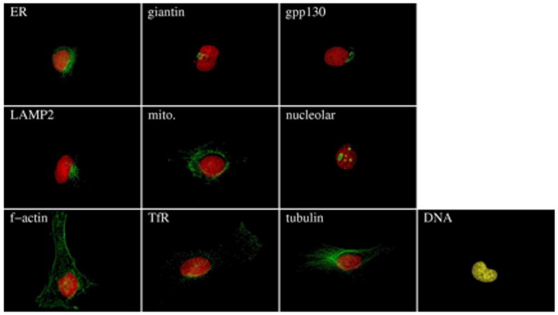
Typical images from the 10-class 2DHELA image dataset. Red color represents DNA staining and green color represents target protein fluorescence.

If the same set of moment and texture features used for the 2D CHO dataset were used for the 2DHeLa dataset, classification accuracy would be expected to be lower since the 2DHeLa set includes twice as many patterns and includes similar classes. Therefore, we developed new sets of features, which included morphological and geometrical features, edge features and DNA features. As shown in Table 2, promising initial results were obtained with feature sets SLF2, SLF4 and SLF5 (2). Even better results have subsequently been obtained by improving the feature sets and using different types of classifiers. The best results obtained to date have been for feature set SLF16 using a mixture-of-experts classifier (6). The results for this classifier are shown in Table 3 in the form of a confusion matrix, where the diagonal shows the accuracies for each individual class and the off-diagonal numbers are the percentage of test samples of each “True” class (row heading) that were misclassified as the “Predicted” class (column heading). It can be seen from the results that automated pattern analysis methods are quite capable of recognizing most major classes of subcellular location patterns. Note that the two pairs of patterns most easily confused are the two Golgi proteins (giantin and gpp130) and the endosomal and lysosomal proteins (LAMP2 and TfR). Even though the accuracies for these two pairs of classes are lower than for other classes, the classification accuracy is high considering the amount of similarity between these pairs of classes and the amount of morphological variability within each class.

Table 3.

Confusion matrix for classification of images from the 2DHeLa set with a mixture-of-experts classifier using SLF8 (a set of 32 features selected by stepwise discriminant analysis from SLF7). The results shown are the average percentages (over 10 cross-validation trials) of images in each true class that are classified in each predicted class.

	Predicted Class
True Class	DNA	ER	Gia	Gpp	Lam	Mit	Nuc	Act	TfR	Tub
DNA	99	1	0	0	0	0	0	0	0	0
ER	0	97	0	0	0	2	0	0	0	1
Gia	0	0	91	7	0	0	0	0	2	0
Gpp	0	0	14	82	0	0	2	0	1	0
Lam	0	0	1	0	88	1	0	0	10	0
Mit	0	3	0	0	0	92	0	0	3	3
Nuc	0	0	0	0	0	0	99	0	1	0
Act	0	0	0	0	0	0	0	100	0	0
TfR	0	1	0	0	12	2	0	1	81	2
Tub	1	2	0	0	0	1	0	0	1	95

The average correct classification rate across all classes was 92%. Results from reference (6).

Classification of the 3DHeLa Dataset

With advances in fluorescence microscope technology in the recent years it has become practical and even commonplace to collect 3-dimensional (3D) images of cells. This provides the opportunity to ask whether automated image interpretation methods can perform better if they use 3D images instead of 2D images. To this end, we constructed a high resolution 3D image set of HeLa cells (22), consisting of 50 to 58 single cell images per class for the same set of classes used in the 2DHeLa set. For each image, parallel DNA and total protein images were recorded using different fluorescence probes. Example images of the 3DHeLa set are shown in Figure 3.

Figure 3.

Typical images from 11-class 3DHeLa image dataset. The eleventh (cytoplasmic) pattern is represented by the blue color. Red, blue and green colors represent DNA staining, total protein staining and target protein fluorescence. Projections on the X-Y (top) and the X-Z (bottom) planes are shown. Image © Carnegie Mellon University; used with permission.

Our first approach to the classification of 3D cells utilized a set of 28 morphological features that included 14 features relating the protein distribution to the parallel DNA image. In combination with a BPNN classifier, this set yielded an overall classification accuracy of 91% (22). Using SLF10, a subset of 9 of these features selected by SDA, an overall accuracy of 95% was achieved (6).

Since a parallel DNA image may not always be available, we determined the contribution of the DNA related features to the overall accuracy. When set SLF14 was created by removing the DNA features from SLF9, a significantly lower overall accuracy of 88% was obtained. To see whether the absence of these features could be compensated for with additional features calculated from the protein image, we implemented new sets of 3D features that included edge and Haralick texture features (24). The optimal use of the Haralick texture features requires a choice of the pixel resolution at which they should be calculated, and experiments revealed that this optimum occurred when images were downsampled to 0.4 micron resolution and 256 gray levels. As seen in Table 4, the SLF17 feature set, containing only 7 features selected from the whole set of morphological, edge and texture features, can provide 98% overall classification accuracy (24). This performance suggests that SLF17 is a near optimal feature set for capturing all major subcellular location patterns in HeLa cells. It is worth noting that the results in Table 4 represent the first time that a classifier was able to achieve greater than 95% accuracy in distinguishing giantin and gpp130, two proteins known to be located in slightly different parts of the Golgi apparatus. It is also worth noting that the measured accuracy of distinguishing these two patterns by visual inspection is below 50% (5).

Table 4.

Confusion matrix for classification of images from the 3DHeLa dataset with a BPNN with 20 hidden units using SLF17. The results shown are averages over 10 cross-validation trials.

True Class	Predicted Class
	DNA	ER	Gia	Gpp	LA	Mit	Nuc	Act	TfR	Tub
DNA	98	2	0	0	0	0	0	0	0	0
ER	0	100	0	0	0	0	0	0	0	0
Giantin	0	0	100	0	0	0	0	0	0	0
Gpp130	0	0	0	96	4	0	0	0	0	0
LAMP2	0	0	0	4	95	0	0	0	0	2
Mitochon-dria	0	0	2	0	0	96	0	2	0	0
Nucleolin	0	0	0	0	0	0	100	0	0	0
Actin	0	0	0	0	0	0	0	100	0	0
TfR	0	0	0	0	2	0	0	0	96	2
Tubulin	0	2	0	0	0	0	0	0	0	98

The average correct classification rate across all classes was 98% Results from reference (24).

Unsupervised Learning of Subcellular Location Patterns

One of the ultimate goals for location proteomics is to determine which proteins share the same location pattern. In other words, given a set of proteins, each with multiple image representations, we need to find a partitioning so that proteins in one partition share a single location pattern. This is analogous to clustering genes by their expression patterns in microarray experiments. In both cases, one of the goals of such clustering is to enable the identification of sequence elements that might be shared between members of a cluster. For co-expressed genes, these may be transcriptional enhancers, while for co-located proteins, they may be targeting motifs. Just as there may be indirect control of transcript clusters (i.e., one or more transcript may regulate the transcription of the others in the cluster), so also may targeting of proteins be indirect (proteins in a cluster may bind to each other with only one of them containing a targeting signal). In any case, the first step to understanding these mechanisms on a proteome-wide scale is to identify all high-resolution location patterns and determine which proteins display each.

Subcellular Location Trees

As discussed before, a library of images representing many, if not all, proteins expressed in a given cell type can be obtained by random tagging techniques. A excellent version of this approach is CD-tagging (12), which introduces an internal GFP domain to the tagged protein. CD-tagging has been used to generate a library of over a hundred clones derived from mouse 3T3 cells, each of which expresses a (usually different) tagged protein (25). Three-dimensional images have been collected for many of these clones using spinning disk confocal microscopy (1).

It is a common practice to explore the similarities of sequence or structure among a set of proteins by constructing a phylogenetic tree. The basis of this construction is a measure of the difference (or similarity) in sequence or structure between each pair of proteins. A similar approach can be used to group proteins using their similarity as reflected in subcellular location features. We refer to the trees created by this approach as subcellular location trees (SLTs).

The initial illustration of the principle of a protein SLT was performed using the 10 classes in the 2DHELA dataset and feature set SLF8 (5). The resulting tree revealed that 1) similar location patterns were grouped first (two Golgi proteins, and the pair of lysosomes and endosomes proteins), and 2) the tree was consistent with the biological understanding of these organelle patterns.

The first SLT built for a protein library was constructed for 46 of the randomly tagged 3T3 cell lines obtained by CD-tagging (1). A critical issue in constructing an SLT is how (or whether) to select features from the starting feature set. In our initial study we described one approach to this problem, in which classifiers are trained in an attempt to distinguish all proteins (even though some protein pairs are expected to be indistinguishable) and increasing numbers of features selected by SDA are used. When this approach was used starting from feature set SLF8 and using a neural network classifier, a final set of 10 features was obtained. This set was able to distinguish all 46 proteins with about 70% accuracy, but since some proteins may share a single location pattern this number does not reflect the accuracy with which the fundamental classes can be distinguished. Examination of this tree is somewhat difficult because the exact underlying true cluster structure is not known (otherwise, the clustering procedure would be unnecessary). However, we observed for example, that most nuclear proteins were grouped into two separate clusters. A close examination of images from the two clusters revealed some subtle differences between them which suggested that the method is sensitive enough to properly separate similar but distinct patterns.

More recently, an updated SLT was created on a larger version of the 3D3T3 dataset (26). This version consisted of 90 tagged proteins. The dataset was first screened to eliminate those proteins considered to be too variable in their distribution (using an algorithm described in the next section). The feature set used to construct this SLT included texture features calculated at an experimentally determined optimal pixel resolution (0.5 micron) and gray levels (64). Also, instead of constructing a single SLT on the dataset, which could be sensitive to small variations, we constructed a consensus tree (27). This is done by constructing many trees, each using a randomly selected half of the images for each protein, and keeping track of which branches are conserved across many of these trees. The resulting consensus tree (Figure 4) and representative images for each protein can be viewed through an interactive browser at http://murphylab.web.cmu.edu/services/PSLID/tree.html

Figure 4.

A consensus subcellular location tree generated on the 3D3T3 image dataset. The rows show the name of the tagged protein (where known), the description assigned from visual inspection, and the subcellular location inferred from annotations in the Gene Ontology (GO) database. Names of proteins whose location from visual inspection differs significantly from that inferred from GO annotation are preceeded with **. The sum of length of vertical edges connecting two proteins represents the distance between them. From reference (26).

Objective Grouping of Proteins Based on Subcellular Location Patterns

A traditional difficulty in interpreting tree-structured clustering algorithms is to find which branches represent the same class. An equivalent problem is to find the number of inherent clusters. A parallel approach we used for this problem is to cluster all individual images from all proteins (by k-means algorithm) and determine the optimal number of clusters (by Akaike Information Content). However, some of the clusters contained only outlier images from some proteins. Therefore, we estimated the optimal number of clusters to be the number of clusters containing a majority of the images of at least one protein.

When this method is applied to the 3D3T3 dataset, 17 clusters (excluding those clusters containing only outliers) were obtained. Furthermore, statistical analysis of the partitionings obtained from these two parallel approaches (clustering and cutting the consensus tree to obtain the same number of clusters) revealed a good agreement between them (26), which suggested that either partition largely reflects the real structure for this dataset.

Subcellular Location Trees for analysis of protein targeting mutants

In addition to being useful for location proteomics, SLF features and cluster analysis methods can also be used to determine how many mutant localization phenotypes a particular protein can display. In collaboration with Jack Rohrer’s group at the University of Zurich, we have demonstrated the feasibility of this application by analyzing confocal images of normal and mutant GFP-tagged proteins expressed in HeLa cells (28). A collection of single- and double-mutants in the cytoplasmic tail of a protein (uncovering enzyme, or UCE) that is normally expressed in the trans-Golgi network were created and expressed in HeLa cells. 3D images were collected following the three-color imaging protocol used for the 3DHeLa collection. The images were automatically segmented into single cell regions using the DNA and total protein images, and then SLF were calculated and used to build a hierarchical cluster tree. The value of the approach was demonstrated in that both an intermediate phenotype between the normal and “null” phenotype and an “alternate” phenotype were found; both of these were had not been discerned by visual examination of the images but could be verified once they were identified by the cluster analysis.

Image Comparison

The results reviewed above show that the SLF capture the essential characteristics of protein distributions in fluorescence microscope images. This validates their used for other statistical analyses besides classification and clustering. Following is a brief description of some additional tasks that can be accomplished with the SLF.

Objective Selection of Typical Images

The traditional way of selecting a representative image from an image set is to use visual inspection. However, this process is subjective and labor-intensive. With the numerical SLF available, we can determine the distance of each feature vector (representing an image) to the mean feature vector and images can be ranked by this distance (29). The representative images would be those on top of the ranked list.

Objective Comparison of Two Image Sets

A frequent question asked by biologists about fluorescence image is whether two different image sets represents different location patterns or not. For instance, one could be interested in whether expression of a mutated gene changes the targeted protein location pattern.

To address this problem, we can perform an appropriate multivariate test between the distributions of the SLF of the two image sets. For example, we have used the Hotelling T²-test, which is a multivariate version of the student T-test to compare image sets (30). If the resulting F value from the test is greater than a critical F value calculated from the degrees of freedom at a given confidence level, we conclude that the image sets differ at the given confidence level. By this method, all pairs of classes in 2DHELA dataset were shown to be statistically different at the 95% confidence level, which is consistent with the finding that a trained classifier could distinguish all 10 classes with relatively high accuracy. As a control, two sets of images for cells labeled with different antibodies against the same protein (giantin) were generated and compared. The resulting F value of 1.04 was less than the critical F value of 2.22 at the 95% confidence level (30), demonstrating that this method is not overly sensitive to within class variations.

Software Availability

Much of the software described above is available for download as Matlab and C++ code from http://murphylab.web.cmu.edu/software. Updated versions can be used through the PSLID image database (http://murphylab.web.cmu.edu/services/PSLID), where feature calculation is integrated into the database and inputs to analysis functions are specified as the results of a text- or content-based image query). The PSLID software is also available for local installation.

Conclusions

Location proteomics is an important branch of proteomics because protein location is an essential aspect of protein behavior. Computerized methods for image interpretation are needed for location proteomics since they are efficient, cost-saving, objective and sensitive to subtle differences. In the current review, we have briefly discussed the current advances in the development of subcellular location features for both 2D and 3D protein fluorescence images. We also discussed the automated interpretation methods, including classifiers, clustering algorithms and other statistical analysis tools derived from these numerical descriptors of an image. Combined with advances in random tagging and high-throughput imaging techniques, these computational methods can generate a complete view of the location patterns for most, if not all, proteins expressed in an arbitrary cell type. Encouraging progress in combining automated microscopy with pattern analysis methods has been reported recently (7). While many challenges remain, the first comprehensive and objective grouping of proteins by their high-resolution subcellular location is within reach.

Finally, systems biology efforts to build bottom-up models of complex behaviors at the cellular level and higher will require detailed information on the subcellular location of all proteins. This information will need to be in the form of generative, stochastic models that capture the cell-to-cell variation in patterns within a location cluster, and that can be combined to generate synthetic cell images in which each protein is distributed in accordance with all available data. The development of methods for building generative models of highly variable subcellular patterns will be an important challenge for the field over the next few years.

Figure 1.

Illustration of morphological features extracted from images of two subcellular patterns. Objects are defined using an automated threshold selection method. The size and distance features are measured in pixels.

References

- 1.Chen X, Velliste M, Weinstein S, Jarvik JW, Murphy RF. Location proteomics - Building subcellular location trees from high resolution 3D fluorescence microscope images of randomly-tagged proteins. Proc SPIE. 2003;4962:298–306. [Google Scholar]
- 2.Boland MV, Markey MK, Murphy RF. Automated recognition of patterns characteristic of subcellular structures in fluorescence microscopy images. Cytometry. 1998;33(3):366–375. [PubMed] [Google Scholar]
- 3.Boland MV, Murphy RF. A Neural Network Classifier Capable of Recognizing the Patterns of all Major Subcellular Structures in Fluorescence Microscope Images of HeLa Cells. Bioinformatics. 2001;17(12):1213–1223. doi: 10.1093/bioinformatics/17.12.1213. [DOI] [PubMed] [Google Scholar]
- 4.Danckaert A, Gonzalez-Couto E, Bollondi L, Thompson N, Hayes B. Automated Recognition of Intracellular Organelles in Confocal Microscope Images. Traffic. 2002;3(1):66–73. doi: 10.1034/j.1600-0854.2002.30109.x. [DOI] [PubMed] [Google Scholar]
- 5.Murphy RF, Velliste M, Porreca G. Robust Numerical Features for Description and Classification of Subcellular Location Patterns in Fluorescence Microscope Images. J VLSI Sig Proc. 2003;35(3):311–321. [Google Scholar]
- 6.Huang K, Murphy RF. Boosting Accuracy of Automated Classification of Fluorescence Microscope Images for Location Proteomics. BMC Bioinformatics. 2004;5:78. doi: 10.1186/1471-2105-5-78. [DOI] [PMC free article] [PubMed] [Google Scholar]
- 7.Conrad C, Erfle H, Warnat P, Daigle N, Lorch T, Ellenberg J, Pepperkok R, Eils R. Automatic Identification of Subcellular Phenotypes on Human Cell Arrays. Genome Research. 2004;14:1130–1136. doi: 10.1101/gr.2383804. [DOI] [PMC free article] [PubMed] [Google Scholar]
- 8.Murphy RF. Location proteomics: a systems approach to subcellular location. Biochem Soc Trans. 2005;33:535–538. doi: 10.1042/BST0330535. [DOI] [PubMed] [Google Scholar]
- 9.Hood L, Heath JR, Phelps ME, Lin B. Systems Biology and New Technologies Enable Predictive and Preventative Medicine. Science. 2004;306(5696):640–643. doi: 10.1126/science.1104635. [DOI] [PubMed] [Google Scholar]
- 10.Valet G. Human cytome project, cytomics and systems biology: the incentive for new horizons in cytometry. Cytometry A. 2005;64A(1):1–2. doi: 10.1002/cyto.a.20120. [DOI] [PubMed] [Google Scholar]
- 11.Valet G, Tarnok A. Potential and challenges of a human cytome project. J Biol Regul Homeost Agents. 2004;18(2):87–91. [PubMed] [Google Scholar]
- 12.Jarvik JW, Adler SA, Telmer CA, Subramaniam V, Lopez AJ. CD-Tagging: A new approach to gene and protein discovery and analysis. BioTechniques. 1996;20(5):896–904. doi: 10.2144/96205rr03. [DOI] [PubMed] [Google Scholar]
- 13.Rolls MM, Stein PA, Taylor SS, Ha E, McKeon F, Rapoport TA. A visual screen of a GFP-fusion library identifies a new type of nuclear envelope membrane protein. J Cell Biol. 1999;146(1):29–44. doi: 10.1083/jcb.146.1.29. [DOI] [PMC free article] [PubMed] [Google Scholar]
- 14.Telmer CA, Berget PB, Ballou B, Murphy RF, Jarvik JW. Epitope Tagging Genomic DNA Using a CD-Tagging Tn10 Minitransposon. BioTechniques. 2002;32:422–430. doi: 10.2144/02322rr04. [DOI] [PubMed] [Google Scholar]
- 15.Habeler G, Natter K, Thallinger GG, Crawford ME, Kohlwein SD, Trajanoski Z. YPL. db: the Yeast Protein Localization database. Nucleic Acids Research. 2002;30(1):80–83. doi: 10.1093/nar/30.1.80. [DOI] [PMC free article] [PubMed] [Google Scholar]
- 16.Kumar A, Cheung K-H, Ross-Macdonald P, Coelho PSR, Miller P, Snyder M. TRIPLES: a database of gene function in Saccharomyces cerevisiae. Nucleic Acids Research. 2000;28(1):81–84. doi: 10.1093/nar/28.1.81. [DOI] [PMC free article] [PubMed] [Google Scholar]
- 17.Kumar A, Agarwal S, Heyman JA, Matson S, Heidtman M, Piccirillo S, Umansky L, Drawid A, Jansen R, Liu Y, et al. Subcellular localization of the yeast proteome. Genes Develop. 2002;16:707–719. doi: 10.1101/gad.970902. [DOI] [PMC free article] [PubMed] [Google Scholar]
- 18.Harris MA, Clark J, Ireland A, Lomax J, Ashburner M, Foulger R, Eilbeck K, Lewis S, Marshall B, Mungall C, et al. The Gene Ontology (GO) database and informatics resource. Nucleic Acids Res. 2004;32:D258–D261. doi: 10.1093/nar/gkh036. [DOI] [PMC free article] [PubMed] [Google Scholar]
- 19.Teague MR. Image analysis via the general theory of moments. J Opt Soc Am. 1980;70(8):920–930. [Google Scholar]
- 20.Haralick R, Shanmugam K, Dinstein I. Textural features for image classification. IEEE Trans Systems Man Cybernetics. 1973;SMC-3(6):610–621. [Google Scholar]
- 21.Haralick RM. Statistical and structural approaches to texture. Proc IEEE. 1979;67(5):786–804. [Google Scholar]
- 22.Velliste M, Murphy RF. Automated Determination of Protein Subcellular Locations from 3D Fluorescence Microscope Images. Proc 2002 IEEE Intl Symp Biomedl Imag (ISBI-2002) 2002:867–870. [Google Scholar]
- 23.Huang K, Velliste M, Murphy RF. Feature Reduction for Improved Recognition of Subcellular Location Patterns in Fluorescence Microscope Images. Proc SPIE. 2003;4962:307–318. [Google Scholar]
- 24.Chen X, Murphy RF. Robust Classification of Subcellular Location Patterns in High Resolution 3D Fluorescecne Microscopy Images. Proc 26th Intl Conf IEEE Eng Med Biol Soc. 2004:1632–1635. doi: 10.1109/IEMBS.2004.1403494. [DOI] [PubMed] [Google Scholar]
- 25.Jarvik JW, Fisher GW, Shi C, Hennen L, Hauser C, Adler S, Berget PB. In vivo functional proteomics: Mammalian genome annotation using CD-tagging. BioTechniques. 2002;33(4):852–867. doi: 10.2144/02334rr02. [DOI] [PubMed] [Google Scholar]
- 26.Chen X, Murphy RF. Objective Clustering of Proteins Based on Subcellular Location Patterns. Journal of Biomedicine and Biotechnology. 2005;2005(2):87–95. doi: 10.1155/JBB.2005.87. [DOI] [PMC free article] [PubMed] [Google Scholar]
- 27.Theorely JL, Page RDM. RadCon: Phylogenetic tree comparison and consensus. Bioinformatics. 2000;16:486–487. doi: 10.1093/bioinformatics/16.5.486. [DOI] [PubMed] [Google Scholar]
- 28.Nair P, Schaub BE, Huang K, Chen X, Murphy RF, Griffith JM, Geuze HJ, Rohrer J. Characterization of the TGN Exit Signal of the human Mannose 6-Phosphate Uncovering Enzyme. Journal of Cell Science. 2005;118:2949–2956. doi: 10.1242/jcs.02434. [DOI] [PubMed] [Google Scholar]
- 29.Markey MK, Boland MV, Murphy RF. Towards objective selection of representative microscope images. Biophys J. 1999;76(4):2230–2237. doi: 10.1016/S0006-3495(99)77379-0. [DOI] [PMC free article] [PubMed] [Google Scholar]
- 30.Roques EJS, Murphy RF. Objective Evaluation of Differences in Protein Subcellular Distribution. Traffic. 2002;3(1):61–65. doi: 10.1034/j.1600-0854.2002.30108.x. [DOI] [PubMed] [Google Scholar]