Generalized Algorithms for Direct Reconstruction of Parametric Images from Dynamic PET Data

Abstract

Indirect and direct methods have been developed for reconstructing parametric images from dynamic PET data. Indirect methods are simple and easy to implement because reconstruction and kinetic modeling are performed in two separate steps. Direct methods estimate parametric images directly from dynamic PET sinograms and, in theory, can be statistically more efficient, but the algorithms are often difficult to implement and are very specific to the kinetic model being used. This paper presents a class of generalized algorithms for direct reconstruction of parametric images that are relatively easy to implement and can be adapted to different kinetic models. The proposed algorithms use optimization transfer principle to convert the maximization of a penalized likelihood into a pixel-wise weighted least squares (WLS) kinetic fitting problem at each iteration. Thus, it can employ existing WLS algorithms developed for kinetic models. The proposed algorithms resemble the empirical iterative implementation of the indirect approach, but converge to a solution of the direct formulation. Computer simulations showed that the proposed direct reconstruction algorithms are flexible and achieve a better bias-variance tradeoff than indirect reconstruction methods.

I. Introduction

Parametric imaging using dynamic positron emission tomography (PET) provides important information for biological research and clinical diagnosis (e.g. [1]–[3]). To obtain a parametric image, a typical approach is to reconstruct a sequence of emission images from the measured projection data first [4], and then to fit the time activity curve (TAC) at each pixel to a linear or nonlinear kinetic model [5]. To obtain an efficient estimate, the noise distribution of the reconstructed activity images should be modeled in the kinetic analysis. However, exact modeling of the noise distribution in emission images reconstructed by iterative methods is difficult because the noise is spatially variant and object-dependent. Usually the space-variant noise variance and correlations between pixels are simply ignored in the kinetic fitting, which can lead to sub-optimal results.

Direct reconstruction of parametric images from the raw projection data solves this problem by combining kinetic modeling and emission image reconstruction into a single formula. It allows accurate compensation of noise propagation from sinogram to the kinetic fitting process. Direct reconstruction has been given attention by many researchers [6]–[15]. It has been shown that images reconstructed by direct reconstruction methods have better bias-variance characteristics than those obtained by indirect methods for both linear models [13], [14] and nonlinear kinetic models [12], [16], [17].

One drawback of direct reconstruction with compartment models is that the optimization algorithms are usually more complex than indirect methods, because the kinetic parameters are involved in the reconstruction formulation nonlinearly [12], [15]. Carson and Lange [6] and Yan et al [17] used the expectation-maximization framework. Kamasak et al [12] applied the coordinate descent algorithm to dynamic PET reconstruction. Both methods result in nonlinear optimization algorithms that are limited to the specific kinetic model being used.

In this paper we present a new method for direct reconstruction to overcome this difficulty. The proposed method decouples image update and kinetic modeling at each iteration to take advantage of well-developed fitting algorithms for kinetic modeling. By using the optimization transfer principle, the proposed algorithms transfer the penalized maximum likelihood problem at each iteration into a pixel-wise nonlinear least squares (NLS) formulation, which can be easily solved by existing algorithms developed for compartment modeling, such as the Levenberg-Marquardt algorithm for general compartment models [18] and the basis function algorithm for one-tissue compartment models [5], [19], [20]. Therefore, the proposed method can be adapted to different kinetic models as long as an NLS fitting algorithm exists for that model. Furthermore, it also allows us to use different kinetic models for different organs in an image as long as the information about the organ boundaries and the corresponding kinetic models is available before the reconstruction. In practice, the specific kinetic model for a tissue region is often determined by prior kinetic modeling studies. Regional boundaries can be found using coregistered anatomical images from CT or MRI. For regions that do not conform to a kinetic model, we can simply use frame-based TACs. Essentially the proposed direct reconstruction method is as flexible as indirect methods in handling different kinetic models in different regions. An extension of the proposed method to a simplified reference tissue model can be found in [21].

Each iteration of the proposed algorithms essentially consists of two separate steps: reconstruction of dynamic emission images and a pixel-wise weighted NLS kinetic fitting. The algorithms therefore resemble an empirical iterative implementation of the indirect approach (e.g. [22]), but pursues the solution of direct reconstruction. An essential difference between the NLS fitting in the proposed algorithms and the empirical indirect algorithm is that the weighting factor in kinetic fitting is automatically determined by the surrogate function in the proposed algorithms while it is manually chosen by a user in the indirect algorithm.

The rest of the paper is organized as follows. Section II describes the general formulation of the indirect and direct reconstruction methods for dynamic PET data. Section III presents the details of the proposed algorithm under a minorization-maximization framework. Computer simulations to validate the performance of the proposed algorithms are given in Section IV. Conclusions are drawn in Section V.

II. Reconstruction of Parametric Images

A. Indirect Methods

In indirect methods, the reconstruction of emission images and kinetic modeling are treated separately. Efficient algorithms for both image reconstruction and kinetic modeling have been developed.

1) Emission Image Reconstruction

PET data are modeled as a collection of independent Poisson random variables with the expectation ȳ_m in time frame m related to the image x_m through an affine transform [23]–[25],

$${\overline{\mathit{y}}}_m(\mathit{x})=\mathit{P}{\mathit{x}}_m+{\mathit{r}}_m,$$ (1)

where P ∈ IR^n_i×n_j is the detection probability matrix with element (i, j) being the probability of detecting an event originated in voxel j by detector pair i, and r_m ∈ IR^n_i is the expectation of scattered and random events in the mth frame. n_i and n_j are the total number of the detector pairs and voxels, respectively. The above affine model assumes PET scanner operate in a linear range or at least the count-rate dependent effects can be corrected by normalization factors.

The log-likelihood function of the dynamic data set, omitting constants that are independent of x, is

$$\mathcal{L}(\mathit{y}\mid \mathit{x})=\sum _m\sum _i{y}_{im}log{\overline{y}}_{im}(\mathit{x})-{\overline{y}}_{im}(\mathit{x}),$$ (2)

where y = {y_m} denotes the measured dynamic sinogram and x = {x_m} denotes the unknown dynamic image.

The estimation of the dynamic emission images x can be achieved by maximizing a penalized likelihood function¹

$$\widehat{\mathit{x}}=arg\underset{\mathit{x}\ge \mathbf{0}}{max}\mathcal{L}(\mathit{y}\mid \mathit{x})-\beta \mathcal{U}(\mathit{x}),$$ (3)

where U(x) is a roughness penalty and β is the regularization parameter that controls the tradeoff between the resolution and noise. Commonly used penalty functions can be written in the following form [26]

$$\mathcal{U}(\mathit{x})=\sum _m\sum _{s=1}^{n_s}{\psi }_{sm}({[\mathit{D}{\mathit{x}}_m]}_s),$$ (4)

where D ∈ IR^n_s×n_j is a sparse neighborhood differentiation matrix whose sth row has nonzero elements corresponding to the pixels that form the sth clique, and ψ_sm(·) is the potential function defined on the clique in time frame m.

2) Tracer Kinetic Modeling

Tracer kinetic behaviors in dynamic PET are often described by compartmental models which mathematically can be represented by a set of ordinary differential equations [27], [28],

$$\frac{\text{d}}{\text{d}t}\mathit{c}(t)=\mathit{Kc}(t)+\mathit{Lu}(t)$$ (5)

where c(t) is a column vector representing the activity concentration of different tissue compartments at time t, K and L are the kinetic parameter matrices which comprise of various rate constants, and u(t) denotes the system input. The differential equation model (5) can be analytically solved by using the Laplace transform and the solution is

$$\mathit{c}(t)=\mathit{q}(t)\otimes C_{\text{p}}(t)$$ (6)

where “⊗” denotes the convolution operator, q(t) is the impulse response vector and C_p(t) is the tracer concentration in plasma.

For a commonly used two tissue compartment model, c(t) = (C_f (t), C_b(t))^T where the superscript “T” denotes vector or matrix transpose, C_f(t) and C_b(t) are the concentrations in the free and bound compartments; u(t) = C_p(t); $\mathit{K}=\left(\begin{array}{cc}-(k_2+k_3)& k_4\\ k_3& -k_4\end{array}\right)$ and $\mathit{L}=\left(\begin{array}{c}{K}_1\\ 0\end{array}\right)$, where K₁, k₂, k₃, k₄ are the tracer rate constants. The impulse response vector q(t) is given by

$$\mathit{q}(t)=\frac{K_1}{\mathrm{\Delta }\alpha }\left(\begin{array}{cc}{k}_4-{\alpha }_1& {\alpha }_2-k_4\\ k_3& -k_3\end{array}\right)e^{-\mathit{\alpha }(t)},$$ (7)

where Δα = α₂ − α₁ with ${\alpha }_{1,2}=\frac{1}{2}(k_2+k_3+k_4)\mp \frac{1}{2}{[{(k_2+k_3+k_4)}^2-4k_2{k}_4]}^{1/2}$, and e^−α(t) = (e^−α₁t, e^−α₂t)^T.

The quantity that PET measures is the total concentration

$$C_{\text{T}}(t)=(1-f_v){\mathbf{1}}^T\mathit{c}(t)+f_v{C}_{wb}(t),$$ (8)

where 1 is the all-one vector, f_v is the fractional volume of blood in the tissue, and C_wb(t) is the tracer concentration in the whole blood. In practice, PET data are binned into discrete time frames. Thus the measured quantity in frame m is the average concentration

$$z_m(\mathit{\kappa })=\frac{1}{\mathrm{\Delta }{t}_m}{\int }_{t_{m,s}}^{t_{m,e}}{C}_{\text{T}}(\tau )e^{-\lambda \tau }\text{d}\tau ,$$ (9)

where t_m,s and t_m,e denote the start and end time of frame m, respectively, Δt_m ≡ t_m,e − t_m,s, λ is the decay constant of the radiotracer, and κ contains the kinetic parameters to be estimated. For example, κ = [K₁, k₂, k₃, k₄, f_v]^T for the two-tissue compartment model.

Given a measured TAC, ẑ = {ẑ_m}, kinetic analysis is to estimate the rate constants in K and L, and f_v, which is usually accomplished by using an NLS fitting

$$\widehat{\mathit{\kappa }}=arg\underset{\mathit{\kappa }}{min}\sum _m{\gamma }_m{\left({\widehat{z}}_m-z_m(\mathit{\kappa })\right)}^2,$$ (10)

where {γ_m} are the weighting factors. A simple choice of γ_m is Δt_m. A Levenberg-Marquardt algorithm [18] is commonly used to solve (10).

B. Direct Methods

Direct methods combine the kinetic model and image reconstruction into a single formula. Let κ_j denote the kinetic parameters for pixel j and κ = {κ_j}, the log-likelihood function can be written as,

$$\mathcal{L}(\mathit{y}\mid \mathit{\kappa })=\sum _m\sum _i{y}_{im}log{\overline{y}}_{im}(\mathit{\kappa })-{\overline{y}}_{im}(\mathit{\kappa }).$$ (11)

The expectation of the data is now a nonlinear transform of the kinetic parameters κ,

$${\overline{y}}_{im}(\mathit{\kappa })=\sum _j{p}_{ij}{x}_m({\mathit{\kappa }}_j)+r_{im},$$ (12)

where x_m(κ_j) denotes the image intensity at pixel j in frame m due to the kinetic parameters κ_j.

The solution of the direct reconstruction is

$$\widehat{\mathit{\kappa }}=arg\underset{\mathit{\kappa }}{max}\mathrm{\Phi }(\mathit{\kappa }),\mathrm{\Phi }(\mathit{\kappa })=\mathcal{L}(\mathit{y}\mid \mathit{\kappa })-\beta \mathcal{U}(\mathit{\kappa }).$$ (13)

The smoothness penalty U(κ) can be applied either on the kinetic parameters κ or on the time activity curve x_m(κ). Here we apply the penalty on x_m(κ) and use the same penalty function as shown in (4). An important advantage of applying the penalty on x_m(κ) is that it simplifies the reconstruction algorithm so that the proposed methods can directly adopt existing least squares kinetic fitting algorithms. As a result, the proposed methods can incorporate nearly an arbitrary kinetic model (beyond the linear compartment models in Section II.A.2) as long as a weighted least squares fitting algorithm exists for that kinetic model.

III. The Proposed Minorization-Maximization Algorithms

A. Optimization Transfer

This paper develops a class of optimization transfer algorithms [29] for direct reconstruction of parametric images. The basic idea is depicted in Fig. 1. It constructs a surrogate function φ(κ|κⁿ) of the kinetic parameters at the nth iteration which minorizes the original objective function Φ(κ) by satisfying the following two conditions:

$$\phi (\mathit{\kappa }\mid {\mathit{\kappa }}^n)\le \mathrm{\Phi }(\mathit{\kappa }),$$ (14)

$$\phi ({\mathit{\kappa }}^n\mid {\mathit{\kappa }}^n)=\mathrm{\Phi }({\mathit{\kappa }}^n).$$ (15)

Fig. 1.

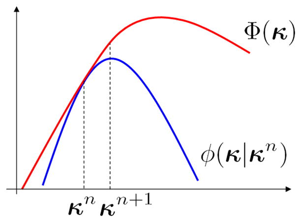
Illustration of optimization transfer. The surrogate function φ(κ|κⁿ) minorizes the original objective function Φ(κ). The new update κⁿ⁺¹ at iteration (n + 1) which is the maxmizer of φ(κ|κⁿ) increases Φ(κ) monotonically.

Throughout this paper, the superscript n denotes the estimate at the nth iteration. Then the maximization of Φ(κ) is transfered into maximizing φ(κ|κⁿ)

$${\mathit{\kappa }}^{n+1}=arg\underset{\mathit{\kappa }}{max}\phi (\mathit{\kappa }\mid {\mathit{\kappa }}^n).$$ (16)

The surrogate function φ(κ|κⁿ) is usually easier to optimize by design than the original objective function. The new update κⁿ⁺¹ increases the original penalized likelihood monotonically,

$$\mathrm{\Phi }({\mathit{\kappa }}^{n+1})\ge \mathrm{\Phi }({\mathit{\kappa }}^n),$$ (17)

and this minorization-maximization procedure guarantees the convergence. The well-known expectation maximization (EM) algorithm [30] is a special case of the optimization transfer algorithms.

B. Paraboloidal Surrogate Function

The Poisson likelihood function can be rewritten in the following form

$$\mathcal{L}(\mathit{y}\mid \mathit{\kappa })=\sum _i\sum _m{h}_{im}(l_{im})$$ (18)

where l_im = [Px_m(κ)]_i and

$$h_{im}(l)=y_{im}log(l+r_{im})-(l+r_{im}).$$ (19)

We use the paraboloidal surrogate function φ^ℒ(κ|κⁿ) that was originally proposed by Fessler and Erdogan in [31] for the log-likelihood function

$$\begin{array}{l}\mathcal{L}(\mathit{y}\mid \mathit{\kappa })\ge {\phi }^{\mathcal{L}}(\mathit{\kappa }\mid {\mathit{\kappa }}^n)\\ =\sum _m\sum _i[h_{im}(l_{im}^n)+{\stackrel{.}{h}}_{im}(l_{im}^n)(l_{im}-l_{im}^n)\\ -\frac{1}{2}{\eta }_{im}(l_{im}^n){(l_{im}-l_{im}^n)}^2]\end{array}$$ (20)

where $l_{im}^n\equiv {[\mathit{P}{\mathit{x}}_m({\mathit{\kappa }}^n)]}_i$ and η_im(l) is the curvature of the surrogate function. Among a few choices, we use the optimal curvature [31]

$${\eta }_{im}(l)=\{\begin{array}{ll}\frac{2}{l^2}[h_{im}(l)-h_{im}(0)-l{\stackrel{.}{h}}_{im}(l)],\hfill & l>0\hfill \\ -{\ddot{h}}_{im}(l),\hfill & l=0\hfill \end{array},$$ (21)

where ḣ_im(l) and ḧ_im(l) are the first and second derivatives of h_im(l), respectively. Note that the paraboloidal surrogate function is only valid for r_im > 0 and l_im ≥ 0.

We also employ the quadratic surrogate function φ^U(κ|κⁿ) that was proposed in [32] to minorize the penalty function at each iteration

$$\begin{array}{l}\mathcal{U}(\mathit{\kappa })\ge {\phi }^{\mathcal{U}}(\mathit{\kappa }\mid {\mathit{\kappa }}^n)\\ =\sum _m\sum _s[{\psi }_{sm}(u_{sm}^n)+{\stackrel{.}{\psi }}_{sm}(u_{sm}^n)(u_{sm}-u_{sm}^n)\\ -\frac{1}{2}{\rho }_{sm}^n{(u_{sm}-u_{sm}^n)}^2]\end{array}$$ (22)

where u_sm ≡ [Dx_m(κ)]_s, $u_{sm}^n\equiv {[\mathit{D}{\mathit{x}}_m({\mathit{\kappa }}^n)]}_s$, and the curvature of the surrogate function for the penalty function, ${\rho }_{sm}^n$, is

$${\rho }_{sm}^n=\frac{{\stackrel{.}{\psi }}_{sm}(u_{sm}^n)}{u_{sm}^n}.$$ (23)

Note that the regularization is applied directly on the emission image x_m(κ).

By combining the surrogate functions for the likelihood and penalty function, the overall surrogate function for the penalized likelihood function in (13) is

$$\begin{array}{l}\phi (\mathit{\kappa }\mid {\mathit{\kappa }}^n)={\phi }^{\mathcal{L}}(\mathit{\kappa }\mid {\mathit{\kappa }}^n)-\beta {\phi }^{\mathcal{U}}(\mathit{\kappa }\mid {\mathit{\kappa }}^n)\\ =\mathrm{\Phi }({\mathit{\kappa }}^n)+\sum _m{({\mathit{g}}_m^n)}^T\mathrm{\Delta }{\mathit{x}}_m-\frac{1}{2}\mathrm{\Delta }{\mathit{x}}_m^T{\mathit{W}}_m^n\mathrm{\Delta }{\mathit{x}}_m,\end{array}$$ (24)

where Δx_m ≡ x_m (κ) − x_m(κⁿ), ${\mathit{g}}_m^n$ denotes the gradient vector and ${\mathit{W}}_m^n$ is the surrogate curvature matrix of the penalized log-likelihood with respect to x at x(κⁿ). They can be calculated by

$${\mathit{g}}_m^n={\mathit{P}}^T\left(\frac{{\mathit{y}}_m}{{\overline{\mathit{y}}}_m({\mathit{\kappa }}^n)}-\mathbf{1}\right)-\beta \text{diag}[{\mathit{\rho }}_m^n]\mathit{D}{\mathit{x}}_m({\mathit{\kappa }}^n)$$ (25)

$${\mathit{W}}_m^n={\mathit{P}}^T\text{diag}[{\mathit{\eta }}_m^n]\mathit{P}+\beta {\mathit{D}}^T\text{diag}[{\mathit{\rho }}_m^n]\mathit{D},$$ (26)

where diag[·] denotes a diagonal matrix, ${\mathit{\eta }}_m^n\equiv {\{{\eta }_{im}(l_{im}^n)\}}_{i=1}^{n_i}$ and ${\mathit{\rho }}_m^n\equiv {\{{\mathit{\rho }}_{sm}^n\}}_{s=1}^{n_s}$.

C. Coordinate Ascent (CA) Algorithm

A pixel-wise coordinate ascent algorithm can be used to maximize the surrogate function φ(κ| κⁿ) to obtain the estimate ${\mathit{\kappa }}_j^{n+1}$. The procedure can be written as

$${\mathit{\kappa }}_j^{n+1}=arg\underset{{\mathit{\kappa }}_j}{max}{\phi }_j({\mathit{\kappa }}_j)$$ (27)

$${\phi }_j({\mathit{\kappa }}_j)=\phi ({\mathit{\kappa }}_1^{n+1},\cdots ,{\mathit{\kappa }}_{j-1}^{n+1},{\mathit{\kappa }}_j,{\mathit{\kappa }}_{j+1}^n,\cdots ,{\mathit{\kappa }}_{n_j}^n\mid {\mathit{\kappa }}^n),$$ (28)

which maximizes φ(κ| κⁿ) for pixel j by fixing other pixels. The above one-dimenstional objective function can be written in a quadratic form

$${\phi }_j({\mathit{\kappa }}_j)=\sum _m{\widehat{g}}_{jm}^n\mathrm{\Delta }{x}_{jm}-\frac{1}{2}{w}_{jm}^n\mathrm{\Delta }{x}_{jm}^2,$$ (29)

where $\mathrm{\Delta }{x}_{jm}\equiv {[\mathrm{\Delta }{\mathit{x}}_m]}_j=x_m({\mathit{\kappa }}_j)-x_m({\mathit{\kappa }}_j^n)$ and the gradient ${\widehat{g}}_{jm}^n$ and curvature $w_{jm}^n$ with respect to x_jm are

$${\widehat{g}}_{jm}^n=g_{jm}^n+\sum _{l<j}{[{\mathit{W}}_m^n]}_{jl}(x_m({\mathit{\kappa }}_l^{n+1})-x_m({\mathit{\kappa }}_l^n)),$$ (30)

$$w_{jm}^n\equiv {[{\mathit{W}}_m^n]}_{jj}=\sum _i{\eta }_{im}^n{p}_{ij}^2+\beta \sum _s{\rho }_{sm}^n{d}_{sj}^2,$$ (31)

with d_sj being the (s, j)th element of D.

Maximizing φ_j(κ_j) with respect to κ_j is then equivalent to the following least squares problem

$${\mathit{\kappa }}_j=arg\underset{{\mathit{\kappa }}_j}{min}\frac{1}{2}\sum _m{w}_{jm}^n{\left(x_m({\mathit{\kappa }}_j)-x_{jm}^{n+1}\right)}^2,$$ (32)

where

$$x_{jm}^{n+1}=x_m({\mathit{\kappa }}_j^n)+\frac{{\widehat{g}}_{jm}^n}{w_{jm}^n}.$$ (33)

Equation (33) can be seen as a coordinate-wise ascent update of the emission image to obtain $x_{jm}^{n+1}$ and (32) is just an NLS fitting with the newly estimated image. Note $w_{jm}^n$ is defined by the surrogate function and compensates for the noise propagation in the kinetic fitting.

D. Separable Paraboloid (SP) Algorithm

The coordinate ascent algorithm requires column-access of the system matrix P, which is difficult to parallelize and incompatible with ordered-subsets method. Using the convex property of φ(κ|κⁿ) in (24), we can construct a separable surrogate φ^s(κ|κⁿ)

$${\phi }^s(\mathit{\kappa }\mid {\mathit{\kappa }}^n)=\sum _m{({\mathit{g}}_m^n)}^T\mathrm{\Delta }{\mathit{x}}_m-\frac{1}{2}\mathrm{\Delta }{\mathit{x}}_m^T\text{diag}[{\widehat{\mathit{w}}}_m^n]\mathrm{\Delta }{\mathit{x}}_m,$$ (34)

where ${\widehat{\mathit{w}}}_m^n={\{{\widehat{w}}_{jm}^n\}}_{j=1}^{n_j}$ is given by

$${\widehat{w}}_{jm}^n=\sum _i{\eta }_{im}^n{p}_{ij}{p}_i+\beta \sum _s{\rho }_{sm}^n{d}_{sj}{d}_j$$ (35)

where p_i ≡ Σ_j p_ij and d_j ≡ Σ_s d_sj. We omit Φ(κⁿ) in (34) for simplicity.

The new surrogate is composed of separable paraboloids [33], [34], which can be maximized for all the pixels simultaneously. Maximizing φ^s(κ| κⁿ) with respect to κ can be written into the following least squares formulation

$${\mathit{\kappa }}_j^{n+1}=arg\underset{{\mathit{\kappa }}_j}{min}\frac{1}{2}\sum _m{\widehat{w}}_{jm}^n{\left(x_m({\mathit{\kappa }}_j)-x_{jm}^{n+1}\right)}^2,$$ (36)

where

$$x_{jm}^{n+1}=x_m({\mathit{\kappa }}_j^n)+\frac{g_{jm}^n}{{\widehat{w}}_{jm}^n},$$ (37)

where $g_{jm}^n$ is the jth element of ${\mathit{g}}_m^n$ defined in (25) and ${\widehat{w}}_{jm}^n$ is given in (35). Equation (37) has the same form as the SP algorithm for emission image reconstruction and (36) can be solved by any NLS algorithm for kinetic modeling.

E. Summary of the Algorithms

In the above algorithms, the minorization step implicitly consists of a dynamic image update procedure. The surrogate function constructed in this step is nonlinear with respect to the kinetic parameters, but is quadratic with respect to the activity image. The maximization step is then solved by a least squares formulation. The minorization-maximization (MM) algorithm can be summarized into the following reconstruction-fitting steps at each iteration:

1. Image reconstruction

   $$x_{jm}^{n+1}=x_m({\mathit{\kappa }}_j^n)+\frac{g_{jm}}{w_{jm}},$$ (38)

2. Weighted NLS fitting

   $${\mathit{\kappa }}_j^{n+1}=arg\underset{{\mathit{\kappa }}_j}{min}\sum _m{w}_{jm}{\left(x_m({\mathit{\kappa }}_j)-x_{jm}^{n+1}\right)}^2,$$ (39)

   where the gradient g_jm equals to ${\widehat{g}}_{jm}^n$ for the CA algorithm and $g_{jm}^n$ for the SP algorithm, and the weighting factor w_jm equal to $w_{jm}^n$ for the CA algorithm and ${\widehat{w}}_{jm}^n$ for the SP algorithm.

The advantage of the proposed algorithms is that they can be adapted to different kinetic models by directly using existing NLS algorithms in the kinetic fitting step. Furthermore, because the kinetic fitting is performed pixel-by-pixel, we can easily apply different kinetic models to different organs in an image if necessary.

It is worth noting that the weights in (39) are determined by the surrogate function and are updated at each outer iteration, as opposed to that the weights in the NLS fitting in indirect methods are often selected empirically by users. Another feature is that it is not necessary to run the NLS fitting in (39) till convergence at each iteration, as long as the new estimate increases the cost function. Here we use two iterations of the Levenberg-Marquardt algorithm [35]. Therefore, each iteration of the direct reconstruction takes about the same amount of time as that for one iteration of the dynamic image reconstruction and two iterations of the Levenberg-Marquardt algorithm.

F. Convergence

Both the CA and SP algorithms are monotonically convergent. However, because of the nonlinear relationship between the dynamic PET data and kinetic parameters, the log-likelihood function ℒ (y|κ) is non-concave with respect to κ. As a result, both algorithms can only guarantee convergence to a local optimum.

IV. Simulation Studies

We performed computer simulations to validate the proposed MM algorithms. The tracer kinetic models include a dynamic ¹⁸F-FDG study with a two-tissue compartment model for imaging glucose metabolism and a dynamic ¹⁵O-water PET study with a one-tissue compartment model for blood flow imaging. The MM algorithm for the FDG study used the CA algorithm with the Levenberg-Marquardt fitting algorithm. The MM algorithm for the water study used the SP algorithm with the basis function algorithm [5], [19], [20] in the fitting step. Both algorithms were implemented in MATLAB. Fifty iterations were used for the CA algorithm and 500 iterations were used for the SP algorithm to ensure effective convergence.

A. Metabolism Imaging with ¹⁸F-FDG PET

A phantom shown in Fig. 2(a) was used to simulate glucose metabolism in brain. It consists of gray matter, white matter and a small tumor inside the white matter. The TAC of each region was generated using a two tissue compartment model and an analytical blood input function in Feng’s model [36]. The calculation of the kinetic model and the fitting procedure were performed using functions provided by the COMKAT package [35]. The kinetic parameters used in the simulation were taken from literature [37] and are listed in Table I. f_v was set to zero for all regions. The scanning schedule of dynamic PET data consists of 30 time frames: 4×20 s, 4×40 s, 4×60 s, 4×180 s and 14×300 s, the same as that used in [37].

Fig. 2.

The FDG-PET simulation settings. (a) A brain phantom composed of gray matter, white matter and a small tumor; (b) the blood input function; and (c) regional time activity curves.

TABLE I.

The kinetic parameters used in the FDG PET simulation.

	K1 min−1	k2 min−1	k3 min−1	k4 min−1
Gray matter	0.1104	0.1910	0.1024	0.0094
White matter	0.0622	0.1248	0.0700	0.0097
Tumor	0.0640	0.0890	0.0738	0.0057

The TACs were integrated for each frame and forward projected to generate dynamic sinograms. Poisson noise was then generated, which resulted in an expected total number of events over the 90 minutes equal to 50 million. One hundred independent and identically-distributed noisy datasets were generated and processed independently by the direct method and indirect method to estimate the kinetic parameters. The regularization parameters in both methods were the same and varied from a reasonably small value 10⁻⁸ to a large value 10⁻⁴. Both methods use the CA algorithm in the reconstruction step and the Levenberg-Marquardt algorithm in the fitting step. The weighting factor in the kinetic fitting in the indirect method was chosen to be the squared frame duration divided by the total number of events in the frame [5]. The computational cost is about 10 s per reconstruction step and 5 s per kinetic fitting step for a total of 15 s per iteration in MATLAB when running on a single 3 GHz CPU. The long reconstruction time of the CA algorithm is mostly due to the inefficiency of MATLAB in handling loops.

The major parameter of interest for FDG PET studies is the influx rate

$$K_i=\frac{K_1{k}_3}{k_2+k_3}$$ (40)

which is related to the glucose metabolic rate by a scaling factor [38]. Fig. 3 shows K_i images reconstructed by the direct method and indirect method. The regularization parameters used in the two methods are the same (β = 10⁻⁵). In comparison, the result of the direct reconstruction is less noisy and the tumor is better defined.

Fig. 3.

Sample images of the influx rate K_i reconstructed using the direct and indirect methods.

The corresponding mean and standard deviation images of the reconstructions in Fig. 3 are shown in Fig. 4. The horizontal profiles through the center of the tumor of the mean and standard deviation images are shown in Fig. 5. The similarity between the mean images indicates that both approaches result in similar resolution and bias. However, the standard deviation of the direct reconstruction is much lower than that of the indirect method. The reduction in noise in this case is almost equivalent to a four-fold increase in PET detection sensitivity.

Fig. 4.

The mean and standard deviation images of K_i image reconstructed using the direct and indirect algorithms. The regularization parameter is β = 10⁻⁵.

Fig. 5.

Horizontal profiles through the tumor of the mean and standard deviation images of K_i shown in Fig. 4.

To further compare the two approaches, we computed the average bias (root mean squares) and variance of the parametric images for all the pixels inside each region. Fig. 6 shows the average bias versus average standard deviation tradeoff curves of the influx rate K_i estimated by the direct and indirect methods for different regions in the brain phantom. The curves are a function of the regularization parameter β with β = 10⁻⁵ for the left start points and β = 10⁻⁸ for the right end points. For all the regions, direct reconstruction results in less variance at any given bias level than the indirect method.

Fig. 6.

The average bias versus standard deviation tradeoff curves of the influx rate K_i reconstructed using the direct and indirect algorithms in different brain regions. Different points on the curves were obtained by varying the regularization parameter.

To take into account of spatial correlation, we also calculated the bias versus standard deviation tradeoff curve for region of interest (ROI) quantification. The ROI was chosen to be the tumor region. The tradeoff curves are plotted in Fig. 7. Compared with the bias-standard deviation plots shown in Fig. 6, the standard deviation is reduced because of the average over the pixels inside the ROI. Again, the standard deviation of the direct reconstruction is less than that of the indirect method at all bias levels.

Fig. 7.

The bias versus standard deviation tradeoff of ROI quantification on K_i images reconstructed using the direct and indirect algorithms.

In all the above reconstructions, we used two iteration of the Levenberg-Marquardt algorithm at each fitting step. To study the effect of the number of the kinetic fitting subiterations on reconstructed images, we reconstructed the same data set shown in Fig. 3 using the direct reconstruction algorithm and running the Levenberg-Marquardt algorithm until convergence at each fitting step (typical 10–20 iterations). Fig. 8 compares the objective functions of the two reconstructions (two subiterations per fitting versus convergent fitting) as a function of the outer iteration. The two curves are quite similar with the difference quickly diminishing after 10 outer iterations. This is because that each kinetic fitting step uses the result of previous fitting as the initial value, so after a few outer iterations, the initial value is fairly close to the optimal solution. Therefore, the number of the kinetic fitting subiterations does not affect final reconstructed images as long as the algorithm is run to convergence.

Fig. 8.

(a) Comparison of the objective functions of the direct reconstruction using two iterations of the Levenberg-Marquardt algorithm per fitting versus running the Levenberg-Marquardt algorithm until convergence at every fitting step as a function of the outer iteration. (b) The difference between the two curves shown in (a).

B. Blood Flow Simulation with ¹⁵O-water PET

To demonstrate the wide applicability of the proposed algorithms, we used a different phantom (Fig. 9(a)) to simulate the ¹⁵O-water PET study. The kinetic model of blood flow is described by

Fig. 9.

The ¹⁵O-water simulation settings. (a) A brain phantom composed of gray matter, white matter, and CSF; (b) the blood input function; and (c) regional time activity curves.

$$C_{\text{T}}(t)=(1-f_v)Fexp(-k_{2}t)\otimes C_{\text{p}}(t)+f_v{C}_{wb}(t),$$ (41)

where F is the flow rate and k₂ is the clearance rate [20]. We used the default Gamma3 function in COMKAT [35] as the blood input function. The kinetic parameters used in the simulation were taken from [39] and are listed in Table II. The dynamic PET scanning sequence consists of 21 frames: 6×5 seconds, 9×10 seconds, and 6×30 seconds, the same as that used in [39]. The blood input and the regional time activity curves are shown in Fig. 9(b) and (c), respectively.

TABLE II.

Kinetic parameters used in the ¹⁵O-water simulation.

	F (min−1)	k2 min−1	fv
Gray matter	0.40	0.42	0.05
White matter	0.20	0.25	0.03

One hundred noisy PET sinograms were generated following the same procedure as described in Section IV-A. The expected total number of events over the 5-minute scan was 5 million. Both the indirect and direct methods use the SP algorithm in image reconstruction and the basis function algorithm [19], [20] in NLS fitting. One hundred basis functions with rate constants log-uniformly distributed from 0.01 to 1.5 were used. The weighting factors in the kinetic fitting in the indirect method were set to be the squared frame durations divided by the total counts of the frame. The advantage of the basis function algorithm over the Levenberg-Marquardt algorithm is that it is much faster for one-tissue compartment models [20]. The computational cost of the SP algorithm is 1.0 second per reconstruction step and 0.7 second per kinetic fitting step for a total of 1.7 s per iteration in MATLAB on a single 3 GHz CPU. The reconstruction time can be further reduced by using ordered subsets and parallel computing techniques.

Fig. 10 plots the averaged bias versus averaged standard deviation of the estimated blood flow in the gray matter and white matter. Similar as the FDG PET study, the direct method produces better bias-variance tradeoff than the indirect method for blood flow quantification, although the relative improvement is slightly less than those shown in Fig. 6.

Fig. 10.

The bias versus standard deviation tradeoff curves of the blood flow image reconstructed using the direct and indirect algorithms. Different points on the curve were obtained by varying the regularization parameter.

V. Conclusions

This paper presents a class of generalized algorithms for direct reconstruction of parametric images from dynamic PET sinograms. The proposed algorithms use paraboloid surrogate functions to transfer the penalized maximum likelihood problem into a pixel-wise weighted nonlinear least squares fitting formulation. The algorithms are easy to implement and can be adapted to different kinetic models. Computer simulations show that the proposed algorithms have better bias versus standard deviation characteristics than conventional indirect methods.

References

- 1.Kordower JH, Emborg ME, Bloch J, Ma SY, Chu YP, Leventhal L, McBride J, Chen EY, Palfi S, Roitberg BZ, Brown WD, Holden JE, Pyzalski R, Taylor MD, Carvey P, Ling ZD, Trono D, Hantraye P, Deglon N, Aebischer P. Neurodegeneration prevented by lentiviral vector delivery of GDNF in primate models of Parkinson’s disease. Science. 2000;290(5492):767–773. doi: 10.1126/science.290.5492.767. [DOI] [PubMed] [Google Scholar]
- 2.Gill SS, Patel NK, Hotton GR, O’Sullivan K, McCarter R, Bunnage M, Brooks DJ, Svendsen CN, Heywood P. Direct brain infusion of glial cell line-derived neurotrophic factor in Parkinson disease. Nature Medicine. 2003;9(5):589–595. doi: 10.1038/nm850. [DOI] [PubMed] [Google Scholar]
- 3.Visser E, Philippens M, Kienhorst L, Kaanders J, Corstens F, de Geus-Oei L, Oyen W. Comparison of tumor volumes derived from glucose metabolic rate maps and SUV maps in dynamic 18F-FDG PET. Journal of Nuclear Medicine. 2008;49(6):892–898. doi: 10.2967/jnumed.107.049585. [DOI] [PubMed] [Google Scholar]
- 4.Li QZ, Asma E, Ahn S, Leahy RM. A fast fully 4-D incremental gradient reconstruction algorithm for list mode PET data. IEEE Transactions on Medical Imaging. 2007;26(1):58–67. doi: 10.1109/TMI.2006.884208. [DOI] [PubMed] [Google Scholar]
- 5.Gunn RN, Lammertsma AA, Hume SP, Cunningham VJ. Parametric imaging of ligand-receptor binding in PET using a simplified reference region model. Neuroimage. 1997;6(4):279–287. doi: 10.1006/nimg.1997.0303. [DOI] [PubMed] [Google Scholar]
- 6.Carson RE, Lange K. The EM parametric image reconstruction algorithm. Journal of America Statistics Association. 1985;80(389):20–22. [Google Scholar]
- 7.Zeng GL, Gullberg GT, Huesman RH. Using linear time-invariant system theory to estimate kinetic parameters directly from projection measurements. IEEE Transactions on Nuclear Science. 1995;42(6):2339–2346. [Google Scholar]
- 8.Matthews J, Bailey D, Price P, Cunningham V. The direct calculation of parametric images from dynamic PET data using maximum-likelihood iterative reconstruction. Physics in Medicine and Biology. 1997;42(6):1155–1173. doi: 10.1088/0031-9155/42/6/012. [DOI] [PubMed] [Google Scholar]
- 9.Reutter BW, Gullberg GT, Huesman RH. Kinetic parameter estimation from attenuated SPECT projection measurements. IEEE Transactions on Nuclear Science. 1998;45(6):3007–3013. [Google Scholar]
- 10.Meikle SR, Matthews JC, Cunningham VJ, Bailey DL, Livieratos L, Jones T, Price P. Parametric image reconstruction using spectral analysis of PET projection data. Physics in Medicine and Biology. 1998;43(3):651–666. doi: 10.1088/0031-9155/43/3/016. [DOI] [PubMed] [Google Scholar]
- 11.Vanzi E, Formiconi AR, Bindi D, Cava GL, Pupi A. Kinetic parameter estimation from renal measurements with a three-headed SPECT system: A simulation study. IEEE Transactions on Medical Imaging. 2004;23(3):363–373. doi: 10.1109/TMI.2004.824149. [DOI] [PubMed] [Google Scholar]
- 12.Kamasak ME, Bouman CA, Morris ED, Sauer K. Direct reconstruction of kinetic parameter images from dynamic PET data. IEEE Transactions on Medical Imaging. 2005;24(5):636–650. doi: 10.1109/TMI.2005.845317. [DOI] [PubMed] [Google Scholar]
- 13.Wang GB, Fu L, Qi JY. Maximum a posteriori reconstruction of the patlak parametric image from sinograms in dynamic PET. Physics in Medicine and Biology. 2008;53(3):593–604. doi: 10.1088/0031-9155/53/3/006. [DOI] [PubMed] [Google Scholar]
- 14.Tsoumpas C, Turkheimer FE, Thielemans K. Study of direct and indirect parametric estimation methods of linear models in dynamic positron emission tomography. Medical Physics. 2008;35(4):1299–1309. doi: 10.1118/1.2885369. [DOI] [PubMed] [Google Scholar]
- 15.Tsoumpas C, Turkheimer FE, Thielemans K. A survey of approaches for direct parametric image reconstruction in emission tomography. Medical Physics. 2008;35(9):3963–3971. doi: 10.1118/1.2966349. [DOI] [PubMed] [Google Scholar]
- 16.Wang G, Qi J. Iterative nonlinear least squares algorithms for direct reconstruction of parametric images from dynamic PET. IEEE International Symposium on Biomedical Imaging (ISBI’ 08); 2008. pp. 1031–1034. [Google Scholar]
- 17.Yan J, Wilson BP, Carson RE. Direct 4D list mode parametric reconstruction for PET with a novel EM algorithm. Conference Record of IEEE Nuclear Science Symposium and Medical Imaging Conference; 2008. [DOI] [PMC free article] [PubMed] [Google Scholar]
- 18.Marquardt DW. An algorithm for least-squares estimation of nonlinear parameters. Journal of the Society for Industrial and Applied Mathematics. 1963;11(2):431–441. [Google Scholar]
- 19.Watabe H, Jino H, Kawachi N, Teramoto N, Hayashi T, Ohta Y, Iida H. Parametric imaging of myocardial blood flow with O-15-water and PET using the basis function method. Journal of Nuclear Medicine. 2005;46(7):1219–1224. [PubMed] [Google Scholar]
- 20.Boellaard R, Knaapen P, Rijbroek A, Luurtsema GJJ, Lammertsma AA. Evaluation of basis function and linear least squares methods for generating parametric blood flow images using o-15-water and positron emission tomography. Molecular Imaging and Biology. 2005;7(4):273–285. doi: 10.1007/s11307-005-0007-2. [DOI] [PubMed] [Google Scholar]
- 21.Wang G, Qi J. Direct reconstruction of PET receptor binding parametric images using a simplified reference tissue model. Proc of SPIE. 2009;7258:72580V1–V8. [Google Scholar]
- 22.Reader AJ, Matthews JC, Sureau FC, et al. Iterative kinetic parameter estimation within fully 4D PET image reconstruction. IEEE Nucleal Science Symposium and Medical Imaging Conference. 2006;3:1752–1756. [Google Scholar]
- 23.Ollinger JM, Fessler JA. Positron-emission tomography. IEEE Signal Processing Magazine. 1997;14(1):43–55. 76. [Google Scholar]
- 24.Lewitt RM, Matej S. Overview of methods for image reconstruction from projections in emission computed tomography. Proceedings of the IEEE. 2003;91(10):1588–1611. [Google Scholar]
- 25.Leahy RM, Qi JY. Statistical approaches in quantitative positron emission tomography. Statistics and Computing. 2000;10(2):147–165. [Google Scholar]
- 26.Fessler JA, Booth SD. Conjugate-gradient preconditioning methods for shift-variant PET image reconstruction. IEEE Transactions on Image Processing. 1999;8(5):688–699. doi: 10.1109/83.760336. [DOI] [PubMed] [Google Scholar]
- 27.Schmidt KC, Turkheimer FE. Kinetic modeling in positron emission tomography. Quarterly Journal of Nuclear Medicine. 2002;46(1):70–85. [PubMed] [Google Scholar]
- 28.Gunn RN, Gunn SR, Cunningham VJ. Positron emission tomography compartmental models. Journal of Cerebral Blood Flow and Metabolism. 2001;21(6):635–652. doi: 10.1097/00004647-200106000-00002. [DOI] [PubMed] [Google Scholar]
- 29.Lange K, Hunter DR, Yang I. Optimization transfer using surrogate objective functions. Journal of Computational and Graphical Statistics. 2000;9(1):1–20. [Google Scholar]
- 30.Dempster AP, Laird NM, Rubin DB. Maximum likelihood from incomplete data via the EM algorithm. Journal of the Royal Statistical Society, Series B. 1977;39(1):1–38. [Google Scholar]
- 31.Fessler JA, Erdogan H. A paraboloidal surrogates algorithm for convergent penalized-likelihood emission image reconstruction. IEEE Nuclear Science Syposium and Medical Imaging Conference. 1998;2:1132–5. [Google Scholar]
- 32.Erdogan H, Fessler JA. Monotonic algorithms for transmission tomography. IEEE Transactions on Medical Imaging. 1999;18(9):801–814. doi: 10.1109/42.802758. [DOI] [PubMed] [Google Scholar]
- 33.Erdogan H, Fessler JA. Ordered subsets algorithms for transmission tomography. Physics in Medicine and Biology. 1999;44(11):2835–2851. doi: 10.1088/0031-9155/44/11/311. [DOI] [PubMed] [Google Scholar]
- 34.Ahn S, Fessler JA. Globally convergent image reconstruction for emission tomography using relaxed ordered subsets algorithms. IEEE Transactions on Medical Imaging. 2003;22(5):613–626. doi: 10.1109/TMI.2003.812251. [DOI] [PubMed] [Google Scholar]
- 35.Muzic RF, Cornelius S. Comkat: Compartment model kinetic analysis tool. Journal of Nuclear Medicine. 2001;42(4):636–645. [PubMed] [Google Scholar]
- 36.Feng DG, Wong KP, Wu CM, Siu WC. A technique for extracting physiological parameters and the required input function simultaneously from PET image measurements: Theory and simulation study. IEEE Transactions on Information Technology in Biomedicine. 1997;1(4):243–254. doi: 10.1109/4233.681168. [DOI] [PubMed] [Google Scholar]
- 37.OSullivan F, Saha A. Use of ridge regression for improved estimation of kinetic constants from PET data. IEEE Transactions on Medical Imaging. 1999;18(2):115–125. doi: 10.1109/42.759111. [DOI] [PubMed] [Google Scholar]
- 38.Huang SC, Phelps ME, Hoffman EJ, Kuhl DE. Error sensitivity of fluorodeoxyglucose method for measurement of cerebral metabolic-rate of glucose. Journal of Cerebral Blood Flow and Metabolism. 1981;1(4):391–401. doi: 10.1038/jcbfm.1981.43. [DOI] [PubMed] [Google Scholar]
- 39.Zhou Y, Huang SC, Bergsneider M. Linear ridge regression with spatial constraint for generation of parametric images in dynamic positron emission tomography studies. IEEE Transactions on Nuclear Science. 2001;48(1):125–130. [Google Scholar]