Abstract
Purpose: A simplified linear model approach was proposed to accurately model the response of a flat panel detector used for breast CT (bCT).
Methods: Individual detector pixel mean and variance were measured from bCT projection images acquired both in air and with a polyethylene cylinder, with the detector operating in both fixed low gain and dynamic gain mode. Once the coefficients of the linear model are determined, the fractional additive noise can be used as a quantitative metric to evaluate the system’s efficiency in utilizing x-ray photons, including the performance of different gain modes of the detector.
Results: Fractional additive noise increases as the object thickness increases or as the radiation dose to the detector decreases. For bCT scan techniques on the UC Davis prototype scanner (80 kVp, 500 views total, 30 frames∕s), in the low gain mode, additive noise contributes 21% of the total pixel noise variance for a 10 cm object and 44% for a 17 cm object. With the dynamic gain mode, additive noise only represents approximately 2.6% of the total pixel noise variance for a 10 cm object and 7.3% for a 17 cm object.
Conclusions: The existence of the signal-independent additive noise is the primary cause for a quadratic relationship between bCT noise variance and the inverse of radiation dose at the detector. With the knowledge of the additive noise contribution to experimentally acquired images, system modifications can be made to reduce the impact of additive noise and improve the quantum noise efficiency of the bCT system.
Keywords: noise variance, additive noise, flat panel detector, cone-beam, computerized tomography (CT)
INTRODUCTION
Due to the critical role that the flat panel detector has on cone-beam CT image quality, knowledge of the basic statistical performance from each detector element in a flat panel detector is important. Rabbani and Van Metter1 first proposed the methodology using linear models to analyze the statistics of x-ray detectors. Siewerdsen et al.2 studied the signal and noise performance of an indirect flat panel detector using a linear cascade model. Their model is robust and provides useful information for detectors with a wide range of energies, x-ray converters, modes of operation, and array designs. In their generalized results, the individual pixel mean and variance are both linear functions of the incident exposure. Instead of analyzing the image in frequency domain, a different approach, referred to as the “mean-variance” approach,3, 4 utilizes the first and second order statistics of the detector output based on linear assumptions. Burgess5 investigated the noise variance of a digital mammography system and proposed that the variance of a single image, when calculated from regions of interest (ROIs), has a second order relationship with the incident exposure. Similar observations were also made by Ravaglia et al.6 Yadava et al.7 proposed, using an exposure-equivalent metric, the instrumentation noise-equivalent exposure (INEE) to measure the additive noise for x-ray imaging systems. This model assumes that the signal mean and variance are both linear functions of the incident exposure, with the mean and variance calculated from ROIs. Whiting et al.8 investigated the spectral effect of an energy integrating detector and concluded that the measured detector signal follows a compound Poisson distribution. They also pointed out that the first and second order moments will be directly proportional to the signal mean and variance, respectively. As discussed in all of these studies, there exists a signal-independent noise component , which is represented as the intercept for the linear (or quadratic) relationship between the signal variance (either from an individual pixel or a ROI) and the incident exposure.
As one of the intrinsic properties of an x-ray detector, additive noise affects the overall noise levels, especially when the x-ray signal level is relatively low. The breast CT (bCT) application is a very typical example of cone-beam CT where low dose operation is required to keep the radiation dose to the breast low. In a study by Roos et al.,9 the additive noise from a Varian 4030CB flat panel detector was measured as the standard deviation by subtracting two offset (no x rays) images using the entire detector as the ROI. The additive noise measured showed dependencies on interpixel variance from different gain modes, with values of 4.37 analog to digital units (ADU) for a fixed high gain mode and 3.14 ADU for a fixed low gain mode. In a previous study,10 the additive noise variance of the same detector used in the bCT application was measured from 500 offset (no x rays) images as 15.1±1.3 ADU2 for the entire detector in the fixed low gain mode and 20.7±2.2 ADU2 in the fixed high gain mode. In that study, due to different experimental conditions, it was difficult to confirm the results with those extrapolated from measurements using x-ray exposure. However, that study clearly demonstrated that after the logarithmic preprocessing required for reconstruction, there exists a quadratic relationship between the image noise variance and the inverse of the incident kerma at the detector. The presence of additive electronic noise is the primary cause of this quadratic relationship.11 There are several key questions left unanswered from that study, including why the additive noise could not be consistently extrapolated from measurements using x-ray exposure, and what is the exact expression of the fit coefficients for the quadratic relationship?
The purpose of this study was first to explore a consistent experimental approach to evaluate the linear components of the mean signal and variance for a flat panel detector, with the bCT application driving the need for low dose, low noise flat panel performance. Following previous efforts,10 the effects of different experimental conditions on the measured results were then examined. The efficacy of the dynamic mode of a Varian PaxScan detector in reducing additive noise contribution was also demonstrated.
METHODS AND MATERIALS
Experimental setup and data analysis
The experiments were conducted on the second prototype bCT scanner built in our laboratory, codename “Bodega.” The x-ray focal spot was located 511 mm from the isocenter and 1037 mm from the detector plane. Projection images were acquired using a CsI based flat panel detector system (PaxScan 4030CB, Varian Medical Systems, Palo Alto, CA) with the rotating bCT gantry kept stationary. The detector panel used a layer of 600 μm columnar CsI(Tl) scintillator (with a nominal density of 4.51 g∕cm3) over amorphous silicon TFT arrays. This detector operated in a 2×2 pixel binning mode (388×388 μm2 detector element size) with 1024×768 pixels per frame at 30 frames∕s. Two different gain modes are currently available at this frame rate and pixel binning setting: Fixed low gain and dynamic gain (detailed in Sec. 2C).
As studied previously,10 image lag will affect the measured signal mean and variance. To avoid the impact from image lag, each acquisition set was performed at least 20 min apart from each other. An 18 s “preacquisition” radiation exposure was also applied to the detector immediately before the start of each acquisition set. This allowed charge trapping (i.e., signal build-up phenomenon which is a component of lag) to reach a relative steady state or lag equilibrium operation mode. Five hundred projection images were acquired for each set and confirmed to be in the “lag equilibrium” stage (the pixel mean and variance remain constant through these 500 images). Different air kerma levels were studied by adjusting the tube current (mA) from 1 to 7 mA at 80 kVp. The air kerma level for each measurement was determined at the isocenter with no object present and then converted to the incident kerma on the detector surface (at the central ray) using the inverse square law.
To confirm that the x-ray source fluctuation was not an appreciable component of noise, fluctuation in the x-ray source output was measured using an experimental real time x-ray meter (DISC: JB-1) from Diagnostic Imaging Specialists Corporation (St. Malo, Manitoba, Canada). X-ray flux was measured at different tube currents (1, 3, 5, and 7 mA) with different data sampling rates (30, 100, and 1000 Hz). The standard deviation and mean of the probe output were recorded.
In addition to acquiring projection images without any object in the field of view, a 156 mm diameter polyethylene cylinder was placed at the isocenter of the scanner and was used as the surrogate material for breast adipose tissue. Identical acquisition methods were used as with the air-only images, including kVp, waiting time, preradiation procedure, and air kerma levels emitted from the x-ray tube.
The individual pixel mean [in the gray scale (GS) unit or ADU of the device] and variance (in the unit of GS2 or ADU2) were calculated from 500 repeated measurements at each air kerma level. The mean and variance were calculated for each individual pixel over the temporal acquisition, instead of from spatial ROIs. Linear regression was applied to the calculated pixel mean and variance as a function of the incident air kerma. The determined coefficients were studied using a linear model approach described in Sec. 2B.
Linear models for signal mean and variance
Linear models for the individual pixel mean m(X) and variance v(X) can be derived from a previous work10 and described in a simpler form as
| (1a) |
| (1b) |
where X is the incident x-ray air kerma measured in the detector plane. g is a measure of the overall gain of a linear detector and is determined by the gain mode of the detector. p is a measure of the overall system offset. h reflects the linear property of the pixel variance and is influenced by the gain mode of the detector. The parameter n is a signal and air kerma independent term in the variance, and ideally is equal to the additive noise variance .
Equation 1 is generic for different acquisition conditions, with and without an object. Ideally, with the presence of an object, the coefficients will be
| (2) |
Only g will be modulated by the attenuation of the object. The other three coefficients, p, h, and n, remain constant.
For simplicity, the linear attenuation coefficient of polyethylene at 51 keV (μ=0.19 cm−1) was used, corresponding to the effective energy of the x-ray spectrum used in the bCT system (80 kVp spectrum with 0.2 mm Cu filtration, with a HVL of 5.01 mm Al and a second HVL of 11.45 mm Al).
The scatter and beam hardening caused from the object were not explicitly modeled here and were rather treated as part of the linear model. As shown by Whiting et al.,8 for energy integrating detectors, the signal will follow a “compound Poisson” distribution and the linear relationship between the signal mean and variance will still hold. Thus, beam hardening will not affect the linear model presented in this study. Due to the heavily filtered spectrum and low density object (polyethylene) involved in this study, beam hardening can only affect the accuracy very slightly when comparing gobj=gair⋅e−μt. Similarly, the linear relationship between signal mean and variance is not affected by scatter and a simple derivation is presented in Appendix A. The impact from beam hardening and scatter on the linear coefficients was evaluated from the measured results and was shown to have minimal effect on the linear model, as described in Sec. 3.
Major goals of this study were to verify the simplified linear model described above using experimentally measured data and to explore the optimal experimental condition when the linear coefficient .
Detector gain modes
In this study, two different detector gain modes were compared: Fixed low gain mode and dynamic gain mode. Dynamic gain mode is a combination of fixed low gain (with an integration capacitor of 4 pF for each element) and fixed high gain (with an integration capacitor of 0.5 pF for each element),9 depending on the signal level and a preset threshold value set by the manufacturer. The gain mode used for each pixel is encoded in the 15th bit. With the current bCT system setup in dynamic gain mode, detector elements switch from fixed high gain to fixed low gain mode at the air kerma level of 2.04±0.46 μGy per frame (measured at the detector plane). When operated in the dynamic gain mode, the detector element will use a high gain if the signal level is below the threshold setting, and will switch to low gain mode when the signal level exceeds the threshold. When low gain is used, the 15th bit on this 14 bit system is switched to “1.” When an individual detector element is operating in high gain mode, its response parameters will be different from the fixed low gain, especially for g and h in Eq. 1. With the dynamic gain mode, the acquired air-only images will automatically switch to fixed low gain mode, and therefore it is reasonable to compare the fitting parameters measured from the polyethylene cylinder images, where the acquired polyethylene cylinder images in dynamic gain mode will be comprised of both low gain and high gain regions. Only detector elements within high gain regions were compared to fixed low gain mode.
Fractional additive noise
With an accurate measurement of the additive noise variance using the proposed linear model, “fractional additive noise” λ(X,t) can be determined in 3 by computing the fraction of additive noise variance over the total pixel noise variance
| (3a) |
By using the assumptions from Eq. 2, we have
| (3b) |
As shown in Eq. 3b, the fractional additive noise λ(X,t) is determined by the detector gain gair and hair, the incident air kerma X, the attenuation from the object (photon path length through a different part of the object t), and the additive noise variance . Thus, with the detector response parameters accurately measured, λ(X,t) can be predicted for different detector modes, object sizes, and scan techniques.
It is worth noting that as a similar parameter to describe the effect of additive noise, INEE (Ref. 7) is a special case to determine the air kerma or exposure X when λ(X,t=0)=0.5. One advantage of using fractional additive noise is that it covers different imaging situations based on the targeted object properties.
Quadratic relationship for CT noise variance
With the linear model established in Sec. 2B., the quadratic relationship between bCT noise variance and the inverse of radiation dose (proportional to the incident air kerma for projection acquisition) can be quantitatively confirmed with experimental results. Based on the propagation of uncertainties, a previous study10 derived that after the logarithmic preprocessing used prior to CT reconstruction, the pixel variance will be determined by
| (4) |
A detailed derivation is also presented in Appendix B.
Together with Eq. 1, we have
| (5a) |
By using the assumptions from Eq. 2, we have
| (5b) |
We will demonstrate the utility of the above quadratic relationship below, with experimentally measured data, for explicitly determining various coefficients.
RESULTS
X-ray source fluctuation
To confirm that the x-ray source fluctuation was not an appreciable component of noise, the percentage error=standard deviation∕mean calculated from the probe output were 0.39%±0.06%, 0.25%±0.04%, 0.21%±0.01%, and 0.16%±0.02% for air kerma levels of 1.06, 3.29, 5.52, and 7.76 μGy, respectively. This also included the uncertainty from the probe itself. We confirmed the noise measured in this study was not dominated by the x-ray generator noise.
Linear model coefficients
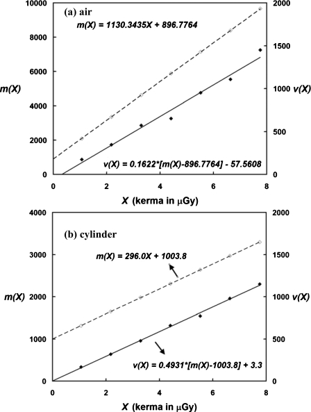
Figure 1 shows the measured mean m(X) and variance v(X) of an individual detector element, as functions of the incident air kerma, with Fig. 1a measured in air and Fig. 1b measured with a polyethylene cylinder, using fixed low gain mode. Linear regression was applied to both the mean and variance for each case. The slopes and intercepts from these linear fits were analyzed using the linear model described in Eq. 1 and recorded for this detector pixel as g, p, h, and n, respectively.
Figure 1.
Linear responses of an individual detector element. Measured mean m(X) and variance v(X) of an individual detector element are shown as functions of the incident air kerma X, measured (a) in air and (b) with a cylinder object, using fixed low gain mode. Measured mean m(X) are shown in hollow diamond markers with dashed lines. Measured variance v(X) are shown in solid diamond markers with solid lines. The slope and intercept of each fitting were recorded for linear model analysis.
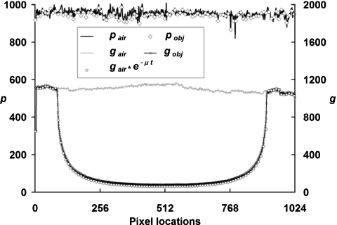
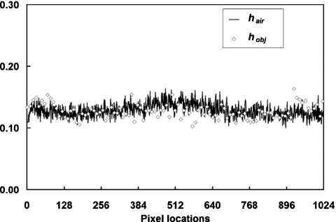
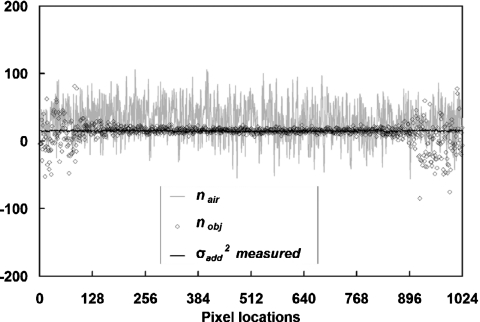
Figures 234 show the linear model coefficients from a single row of detector pixels when the detector was operating in the fixed low gain mode. Coefficients shown in these figures were determined for each individual pixel as described above. The physical pattern of the detector design can also be demonstrated with these coefficients, e.g., gair shown in Fig. 2 depicts the total gain differences among one row of detector pixels. The relationship defined in Eq. 2 can be confirmed with the data shown in these figures.
Figure 2.
Linear coefficients for detector pixel mean. Linear fitting coefficients (gair and gobj for the slope; pair and pobj for the intercept) for detector pixel means measured from projection images acquired in air and with a cylinder object are shown at different pixel locations in a single row of the detector. The detector was in fixed low gain mode. To avoid extensive data points overlapping, gair*e−μt was only shown for every ten pixels. The data clearly demonstrated the following relationships: gobj=gair⋅e−μt, pobj=pair.
Figure 3.
Slopes for pixel variances. Linear fitting slopes for pixel variances measured from projection images acquired in air (hair) and with a cylinder object (hobj) are shown at different pixel locations in a single row of the detector. The detector was in fixed low gain mode. The data clearly demonstrated the following relationship: hobj=hair.
Figure 4.
Intercepts for pixel variances. Linear fitting intercepts for pixel variances measured from projection images acquired in air (nair) and with a cylinder object (nobj) are shown at different pixel locations in a single row of the detector. The detector was in fixed low gain mode. Pixel variances measured directly from dark images are also shown. From this figure, it can be clearly seen that with the presence of the object, the fitting intercepts converge to the additive noise variance measured directly from dark images. For air-only measurements, however, the fitting intercepts greatly fluctuate around the measured additive noise.
In Fig. 2, the proposed linear model for pixel mean can be consistently determined by two coefficients, g and p. The presence of a cylinder object only modulates the slope g by the attenuation from Beer’s law. As confirmed from the measured data, scatter and beam hardening do not have significant impact on these coefficients.
In Fig. 3, the slope h of the linear model for pixel variance is shown for both air and cylinder acquisitions. Due to the definition in Eq. 1, h is also signal-independent and is not affected by the presence of the cylinder object.
In Fig. 4, the intercept n of the linear model for pixel variance is shown for both air and cylinder acquisitions, together with the additive noise variance measured directly from offset images (as measured from previous study,10 the additive noise variance was 15.1±1.3 ADU2 for the entire detector). The intercept nair shows a very large fluctuation, while the intercept nobj converges to the additive noise measured from offset images, in the pixel regions where the object’s shadow can be seen.
The above finding is very important and demonstrates the key challenge of using the linear regression approach to measure the additive noise term. From the linear model of pixel variance, the fluctuation of the measured total pixel variance can be determined together with the fluctuation of the pixel mean part [h[m(X)−p] in Eq. 1] and the additive noise part n. If any data point used in linear regression is measured at a signal level that causes a much larger fluctuation than the additive noise does, the intercept n can no longer be accurately determined from linear regression. Thus, the optimal results can only be achieved within a specific signal range where the contributions to the total pixel variance from the signal mean part and additive noise part are in comparable magnitude. As clearly shown in Fig. 4, since the signal variance measured with the presence of the object is much lower than that measured in air, and is thus closer to the same approximate amplitude as the additive noise, the measured intercept n converges much better to the measured additive noise from offset images.
For the results measured only in air near the edges of Fig. 4, the signal fluctuation dominates and the additive noise is too small to be accurately determined.
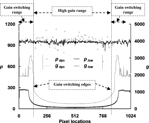
Different detector gain modes
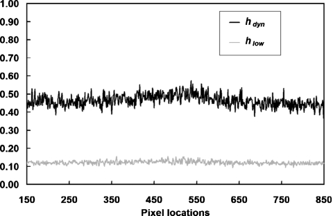
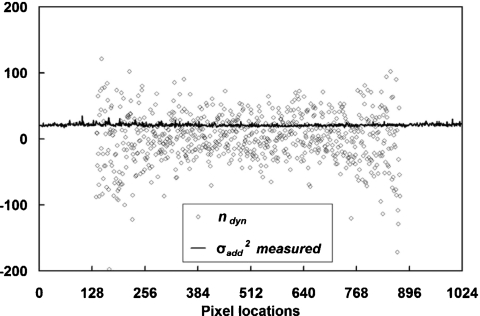
As shown in Figs. 567, the detector response parameters were compared between fixed low gain and dynamic gain modes. The data in Figs. 56 clearly show an increase in the system gain (g and h) when the detector elements use a higher gain with dynamic gain mode. In Fig. 5, the intercept of pixel mean p does not depend on the detector mode. Figure 7 shows a large fluctuation for the intercept of pixel variance ndyn with dynamic gain. This is very similar to the results measured from air images using fixed low gain, as shown in Fig. 4. The cause is also due to the relative small fraction of the additive noise over the overall pixel variance, as discussed in Sec. 3B.
Figure 5.
Linear coefficients for detector pixel mean with different detector gain modes. Linear fitting slope g and intercept p measured using the cylinder object are shown for two different detector modes: (gdyn,pdyn) for dynamic gain and (glow,plow) for fixed low gain. For dynamic gain mode, the detector elements outside of the gain switching edges switched from fixed high gain mode to fixed low gain mode (with the 15th bit set to “1”) during the incremental exposure measurement. Thus, the linear fitting coefficients have a very large fluctuation. Pixels located between #150 and #850 were using a higher gain from the dynamic gain for all the exposure levels. These data show that p does not have a strong dependence on the detector mode.
Figure 6.
Slopes for pixel variance with different detector gain modes. Linear fitting slope h measured using the cylinder object is shown for two different detector modes: hdyn for dynamic gain and hlow for fixed low gain. Pixels located between #150 and #850 were using a higher gain from the linear fitting slope h, measured using the cylinder object, are shown for two different detector modes: hdyn for dynamic gain and hlow for fixed low gain. Pixels located between #150 and #850 were using a higher gain from the dynamic gain and clearly demonstrate a greater slope than fixed low gain.
Figure 7.
Intercepts for pixel variance with dynamic gain mode. Linear fitting intercept ndyn measured using the cylinder object for dynamic gain is shown. For dynamic gain mode, the detector elements around the edge of the object switched to fixed low gain mode. Pixels located between #150 and #850 were using a higher gain from the dynamic gain. A large fluctuation for ndyn is demonstrated compared to measured from offset images.
Fractional additive noise
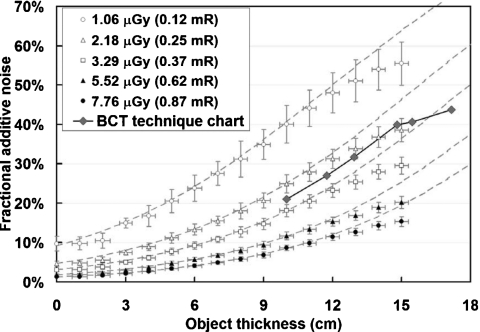
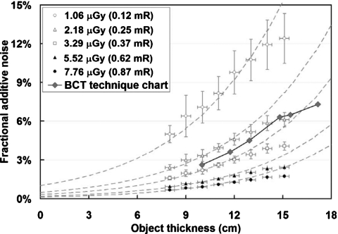
As shown in Figs. 89, the additive noise variance component of the total pixel variance is affected by the object size and the initial incident air kerma for a specific detector mode. The discrete data points in Figs. 89 were calculated from experimentally measured data using Eq. 3a. The results were binned into 1 cm object thicknesses and the mean and standard deviation for each point were also determined from the binning. The dashed lines were computed using the empirical model prediction from Eq. 3b, with fit coefficients and additive noise values measured from offset images. For Fig. 9, because the detector switches to low gain mode when the object thickness is smaller than 8 cm, the high gain component of the dynamic gain mode is only realized when the object thickness is greater than 8 cm. Both Figs. 89 show that the fractional additive noise component increases as the object thickness increases and as the air kerma rate decreases.
Figure 8.
Fractional additive noise with low gain mode. The percentages of additive noise variance in the total pixel noise variance are shown as functions of object thickness and air kerma applied. Fractional additive noise increases as the object thickness increases or as the air kerma level decreases. The discrete data points were calculated from experimentally measured data (binned into 1 cm object thickness; the horizontal error bar shows the thickness distribution within each bin). The dashed lines are from empirical prediction with measured fitting coefficients. For practical bCT scan techniques, additive noise contributes about 21% of the total pixel noise variance for a 10 cm object and 44% for a 17 cm object.
Figure 9.
Fractional additive noise with dynamic gain mode. The fractional additive noise variances in the total pixel noise variance are shown as functions of object thickness and radiation kerma applied. Fractional additive noise increases as the object thickness increases or as the radiation kerma decreases. The discrete data points were calculated from experimentally measured data (binned into 1 cm object thickness; the horizontal error bar shows the thickness distribution within each bin). The dashed lines are from empirical prediction with measured fitting coefficients. For practical bCT scan techniques, additive noise contributes about 2.6% of the total pixel noise variance for a 10 cm object and 7.3% for a 17 cm object.
In Figs. 89, it is worth noting that the discrepancies at larger object thickness between experimentally measured and theoretically calculated data are a result of the continuous attenuation profile of the cylinder phantom. In the case of the cylinder, there were different number of data points used for each thickness bin (binning data from the continuous profile across the cylinder), e.g., there are fewer data points available for larger object thickness. Thus, with the decreasing object gradient toward the center of the object, the binning will bias the results toward smaller object thickness. This explains the “bending over” of the measured data toward the center of the object. Despite this bending over, the overall deviations between experiment and prediction are actually quite small, the largest difference being <1%.
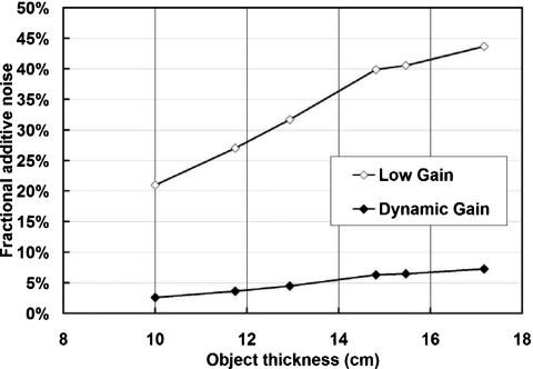
As shown in Fig. 10, for practical bCT scan techniques (500 views total, 30 frames∕s), additive noise contributes about 21% of the total pixel noise variance for a 10 cm object and 44% for a 17 cm object with the fixed low gain mode. When dynamic gain is used, the corresponding fraction drops to 2.6% for a 10 cm object and 7.3% for a 17 cm object.
Figure 10.
Fractional additive noise comparison for bCT. The fractional additive noise variances in the total pixel noise variance are compared between detector modes for practical bCT scan techniques. The corresponding air kerma levels were determined based on the object thickness. With the utilizing of dynamic gain mode, the fractional additive noise decreases by around six times.
As a comparison with previous studies,7, 9 when λ(X,t=0)=0.5, the INEE is 12.06±1.52 μR for the fixed low gain and 0.89±0.11 μR for the fixed high gain. These results demonstrated reasonable accuracy compared to the 15.6 and 1.03 μR values (for fixed low and high gain mode, respectively) measured from a similar detector.9
Quadratic relationship
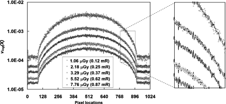
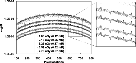
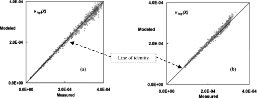
Figures 1112 show the pixel noise variance after logarithmic preprocessing vlog(X) with air kerma levels at different pixel locations in a single row of the detector, with fixed low gain (Fig. 11) and dynamic gain modes (Fig. 12). The discrete data points were calculated from experimentally measured data using Eq. 4. The solid lines (closely overlapped with the discrete data points, as shown in the magnified view on the right side of each figure) were calculated from the empirical prediction using Eq. 5b, with measured fit coefficients and additive noise measured from offset images. Here, the variance after the logarithmic preprocessing step vlog(X) actually equals v(X)∕[m(X)−p]2, and also will be directly proportional to the reconstructed CT noise variance. The concordance between experimental measurement and the theoretical model (shown in Figs. 1112) is demonstrated by the r2 value for each kerma level and detector mode. The computed r2 values were 0.964, 0.981, 0.989, 0.995, and 0.997 for fixed low gain and 0.688, 0.907, 0.958, 0.985, and 0.992 for dynamic gain, for kerma levels of 1.06, 2.18, 3.29, 5.52, and 7.76 μGy, respectively. A lower level of concordance occurred for the dynamic gain with air kerma at 1.06 μGy, where the r2 value was 0.688. The likely reason for this is due to the measurement uncertainty of the pixel variance with very low air kerma. The excellent agreement shown in Figs. 1112 demonstrates that the quadratic relationship described in Eq. 5 is accurate and can be used to explain previous findings related to bCT noise variance.10, 11 Figure 13 also demonstrates the excellent match between experimental data and the theoretical model.
Figure 11.
Pixel variance after logarithmic process with fixed low gain mode. The pixel noise variance after logarithmic preprocessing is shown with different radiation kerma levels at different pixel locations in a single row of the detector. To compensate for the large data range, a logarithmic scale was used for the y-axis. The discrete data points were calculated from experimentally measured data using Eq. 4. The solid lines (closely overlapped with the discrete data points, as shown in the magnified view on the right) were calculated from empirical prediction using Eq. 5b, with measured fitting coefficients and additive noise measured from offset images. These data clearly proved the quadratic relationship described in Eq. 5b.
Figure 12.
Pixel variance after logarithmic process with dynamic gain mode. The pixel noise variance after logarithmic preprocessing is shown with different radiation kerma levels at different pixel locations in a single row of the detector. Only the pixel region with dynamic gain mode was shown (#150–#850). The discrete data points were calculated from experimentally measured data using Eq. 4. The solid lines (closely overlapped with the discrete data points, as shown in the magnified view on the right) were calculated from empirical prediction using Eq. 5b, with measured fitting coefficients and additive noise measured from offset images. These data clearly proved the quadratic relationship described in Eq. 5b.
Figure 13.
Verification of the quadratic relationship. As another way to prove the quadratic relationship from Eq. 5b, the pixel noise variance after logarithmic preprocessing from a single row of the detector were plotted for (a) fixed low gain mode and (b) dynamic gain mode. The air kerma level was 5.52 μGy for a 156 mm polyethylene cylinder. Values from experimental measurements were used as the x-axis and values calculated from the quadratic model in Eq. 5b were used as the y-axis. A very close distribution of the data points around the line of identity verifies that the pixel variance after logarithmic preprocessing is determined by the quadratic relationship from Eq. 5b.
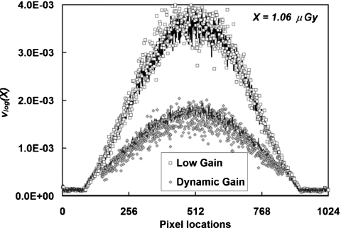
As shown in Fig. 14, when the detector elements operate in the high gain range of the dynamic gain mode, the variance after the logarithmic preprocessing is much lower than when they operate in the fixed low gain mode. For a 156 mm polyethylene cylinder with an incident air kerma of 1.06 μGy (measured in air at the detector plane), the total noise variance decreases by about 50% when using the dynamic gain mode. The polyethylene cylinder phantom used in this study accurately simulates a 100% adipose breast, but for breasts with higher glandularity, the total attenuation would be higher and the fractional additive noise will be accordingly higher.
Figure 14.
Pixel variance comparison between detector modes. The pixel noise variance after logarithmic preprocessing is shown with different detector modes. The air kerma level was 1.06 μGy for a 156 mm polyethylene cylinder. The discrete data points were calculated from experimentally measured data using Eq. 4. The solid lines (closely overlapped with the discrete data points) were calculated from empirical prediction using Eq. 5b, with measured fitting coefficients and additive noise measured from offset images. The pixel noise variance with the dynamic gain mode is only about 50% of that with the fixed low gain mode.
DISCUSSION
Despite the robust and comprehensive nature of the linear cascaded model,2 it is often useful to have a simpler “black box” model, previously referred to as the mean-variance method,3 where only two coefficients are required to determine the linear response (for mean or variance) of each individual pixel. This model may be useful when the numerical values of key parameters of the detector necessary for the linear cascade model are unavailable, such as the internal gain of the electronics, the conversion efficiency, the fill factor of the scintillator, the Poisson excess terms, etc. The coefficients required by the linear model approach proposed here can be simply determined from experimentally acquired images.
As mentioned in Sec. 3B and shown in Figs. 47, to accurately measure the additive noise, the x-ray signal level has to be kept so low that the detector is not working in a quantum limited condition. To “extrapolate” this, it is best to measure additive noise in the absence of x-ray photons, which means using the offset images (no incident x-ray fluence).
In this study, additive noise variance was measured from 500 offset (no x rays) images in the unit of ADU2 as 15.1±1.3 ADU2 for the entire detector in the fixed low gain mode and 20.7±2.2 ADU2 in the fixed high gain mode. For the additive noise standard deviation in the unit of electrons, these results correspond to 5948 electrons in the fixed low gain and 1716 electrons in the fixed high gain, respectively. A detailed conversion is described in Appendix C.
The analysis carried out here leads to an understanding of the noise and signal properties of a CT system up to the point of logarithmic preprocessing. However, after CT reconstruction, the resulting CT voxel variance will be a linear combination of individual projection pixel variances, each of which can be determined by the quadratic equation described in Eqs. 5a, 5b. Thus the fractional additive noise analysis in the projection image will be directly useful for the final CT data. This parameter is more straightforward to predict and easier to evaluate as a function of different system parameters, as shown in Fig. 10 for detector mode comparison.
With the knowledge of the fractional additive noise, practical system modifications can be made to reduce the additive noise contribution in order to improve the quantum efficiency of the bCT system. As shown in this study, using the dynamic gain mode provides a higher external gain of the detector. This will reduce the fractional additive noise since it boosts the signal prior to the injection of additive noise. While the high gain mode has a clear value in the terms of reducing the fractional additive noise, a reduced dynamic range for the detector is a consequence of this approach. Other approaches for system modification are also possible. For example, while keeping the total scan dose constant (equal to or less than a two-view mammography), fewer projection images can be acquired so that the x-ray signal for each view is higher relative to the noise floor. For each individual view, this approach is equivalent to using higher air kerma, as the results in Figs. 891112 demonstrate. This corresponds to a smaller additive noise component for each projection view. With this approach, the tradeoff of the CT image quality when using fewer views has to also be considered.
CONCLUSIONS
In this work, a simplified, non-frequency-dependent, linear model approach was presented, which can be used to accurately model the response of a flat panel detector on a pixel by pixel basis. Under proper experiment conditions, fractional additive noise can be determined using this linear model approach. Once all the coefficients of the linear model were accurately determined, the fractional additive noise can be used as a quantitative metric to better understand an imaging system’s efficiency in utilizing x-ray photons. For appropriate signal amplitudes, the high gain regions of the dynamic gain mode were shown to reduce the fractional additive noise contribution. It was also shown that the signal-independent additive (electronic or thermal) noise is the primary cause for a quadratic relationship between bCT noise variance and the inverse of radiation dose.
ACKNOWLEDGMENTS
The authors would like to thank Dr. Norbert J. Pelc at Stanford University, Dr. Jeffrey H. Siewerdson at Johns Hopkins University, Dr. Bruce R. Whiting at Washington University in St. Louis, and Dr. George Zentai and Dr. Gerhard Roos at Varian, for substantive and meaningful discussions related to additive noise. This work was supported by a grant from the National Institute for Biomedical Imaging and Bioengineering (Grant No. R01 EB002138).
APPENDIX A: LINEAR RELATIONSHIP WITH SCATTER
In this section, we will demonstrate that with scatter, the signal mean and variance still has a linear relationship. As shown by Whiting et al.,8 for energy integrating detectors, if we neglect the additive noise, the primary signal mean and variance of a single detector element are linear to each other
| (A1) |
where κ1 and κ2 are the first and second momentum of the overall summary statistics and determined by
| (A2a) |
| (A2b) |
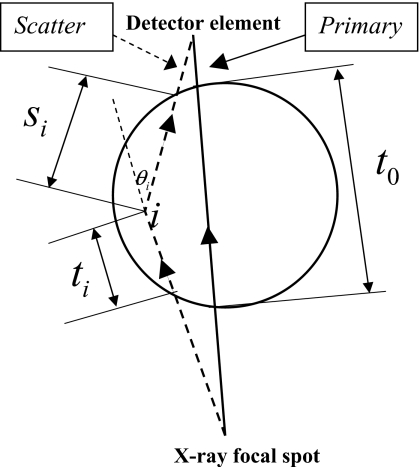
where g(E) is the gain conversion factor for each energy bin of the spectrum. In this study, as shown in Fig. 15, we can first determine gp(E) for primary signal incident onto a single detector element as
| (A3) |
where e−μ(E)t0 is the attenuation through the object and k⋅[1−e−μd(E)td] is from the absorption of the scintillator (CsI) of the detector.
Figure 15.
Appendix A: Linear relationship with scatter. A simple scatter model is shown. A single scatter occurs at voxel i. The scatter angle is θi. t0 is the path length through the object for primary photons and (ti,si) are the path lengths for the scatter photons before and after the scattering.
For a simplified scatter model, we only consider single scatter photons. For an individual scatter beam path that generated at object voxel i, as shown in Fig. 15, the gain conversion factor gs(i,E) can be determined as
| (A4) |
where the Klein–Nishina formula was used to determine the photon energy after scattering and mec2=511 keV is the rest mass of electron. We can determine gs(E) by integrating through the entire object volume for any possible scatter kernel voxel i.
| (A5) |
Thus, the first and second momentum with both primary and scatter signal can be rewritten as
| (A6a) |
| (A6b) |
The signal mean and variance will still hold the same linear relationship as in Eq. A1.
APPENDIX B: VARIANCE AFTER LOGARITHMIC PREPROCESSING STEP
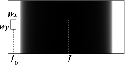
As shown in Fig. 16, the signal from individual detector pixels after offset correction can be treated as a random variable I and each detector element’s statistic properties can be described by the mean and variance . By subtracting the offset level (no x rays) and using the linear model derived in Eq. 1, we have
| (B1a) |
| (B1b) |
As an important initial step for CT reconstruction, the projection image needs to be converted into attenuation path lengths through a logarithmic ratio preprocessing step as ln(I0∕I)=ln I0−ln I, where I0 is the averaged pixel value of a Wx×Wy window from the region of the image where no object is present, as shown in Fig. 16. The mean and variance of this random variable I0 can be written as
| (B2a) |
| (B2b) |
From the mathematics of the noise propagation, the pixel variance after logarithmic preprocessing can be described as
| (B3) |
Since I and I0 are independent measurements from different pixel locations from the image, then
| (B4) |
Inserting Eqs. B2a, B2b, B4 into Eq. B3, we have
| (B5) |
The first term of Eq. B5 can be omitted because Wx and Wy can be relatively large, i.e., the fluctuation from I0 can be minimized using a large averaging window.
Figure 16.
Appendix B: Pixel variance after logarithmic preprocessing. An offset corrected projection image of a cylinder is shown. As an important initial step for CT reconstruction, the projection image needs to be converted into attenuation path lengths through a logarithmic ratio preprocessing step as ln(I0∕I)=ln I0−ln I, where I0 is the averaged pixel value of a Wx×Wy window from the air region of the image.
Thus we have Eq. 4
APPENDIX C: ADDITIVE NOISE IN THE UNIT OF ELECTRONS
We have measured the electronic noise with a standard deviation of 3.9 ADU (variance=15.1 ADU2) for the fixed low gain mode (4 pF, 2× external gain, 2×2 binning) and 4.5 ADU (variance=20.2 ADU2) for the dynamic gain mode (0.5 pF for the high gain part, 1× external gain, 2×2 binning).
As provided by the manufacturer, the detector’s A/D converter is set up to provide 1 ADU∕122 μV. So we can calculate the number of electrons/ADU as
| (C1) |
where conversion factor: f=122×10−6 V∕ADU; feedback capacitance: C=4×10⁻¹² F for fixed low gain or C=0.5×10⁻¹² F for high gain in dynamic gain; external gain of electronics: Gext=2 for fixed low gain or Gext=1 for dynamic gain; internal gain of readout ASIC by design: Gint=0.5; pixel binning gain for 2×2 mode with coupled double sampling: Gbin_CDS=2; and electron charges in Coulomb (C): Q=1.6×10⁻¹⁹ C. For fixed low gain we have
Thus, 3.9 ADU equal to 5948 electrons for the additive noise standard deviation in the fixed low gain mode.
Similarly, for fixed high gain we have
Thus, 4.5 ADU equal to 1716 electrons for the additive noise standard deviation in the fixed high gain mode.
References
- Rabbani M. and Van Metter R., “Analysis of signal and noise propagation for several imaging mechanisms,” J. Opt. Soc. Am. A 6(8), 1156–1164 (1989). 10.1364/JOSAA.6.001156 [DOI] [Google Scholar]
- Siewerdsen J. H., Antonuk L. E., El-Mohri Y., Yorkston J., Huang W., Boudry J. M., and Cunningham I. A., “Empirical and theoretical investigation of the noise performance of indirect detection, active matrix flat-panel imagers (AMFPIs) for diagnostic radiology,” Med. Phys. 24(1), 71–89 (1997). 10.1118/1.597919 [DOI] [PubMed] [Google Scholar]
- Holdsworth D. W., Gerson R. K., and Fenster A., “A time-delay integration charge-coupled device camera for slot-scanned digital radiography,” Med. Phys. 17(5), 876–886 (1990). 10.1118/1.596578 [DOI] [PubMed] [Google Scholar]
- Beecken B. P. and Fossum E. R., “Determination of the conversion gain and the accuracy of its measurement for detector elements and arrays,” Appl. Opt. 35(19), 3471–3477 (1996). 10.1364/AO.35.003471 [DOI] [PubMed] [Google Scholar]
- Burgess A., “On the noise variance of a digital mammography system,” Med. Phys. 31(7), 1987–1995 (2004). 10.1118/1.1758791 [DOI] [PubMed] [Google Scholar]
- Ravaglia V., Bouwman R., Young K., Van Engen R., and Lazzari B., “Noise analysis of full field digital mammography systems,” Proc. SPIE 7258, 72581B–725811 (2009). 10.1117/12.812404 [DOI] [PubMed] [Google Scholar]
- Yadava G. K., Kuhls-Gilcrist A. T., Rudin S., Patel V. K., Hoffmann K. R., and Bednarek D. R., “A practical exposure-equivalent metric for instrumentation noise in x-ray imaging systems,” Phys. Med. Biol. 53(18), 5107–5121 (2008). 10.1088/0031-9155/53/18/017 [DOI] [PMC free article] [PubMed] [Google Scholar]
- Whiting B. R., Massoumzadeh P., Earl O. A., O’Sullivan J. A., Snyder D. L., and Williamson J. F., “Properties of preprocessed sinogram data in x-ray computed tomography,” Med. Phys. 33(9), 3290–3303 (2006). 10.1118/1.2230762 [DOI] [PubMed] [Google Scholar]
- Roos P. G., Colbeth R. E., Mollov I., Munro P., Pavkovich J., Seppi E. J., Shapiro E. G., Tognina C. A., Virshup G. F., Yu J. M., Zentai G., Kaissl W., Matsinos E., Richters J., and Riem H., “Multiple-gain-ranging readout method to extend the dynamic range of amorphous silicon flat-panel imagers,” Proc. SPIE 5368, 139–149 (2004). 10.1117/12.535471 [DOI] [Google Scholar]
- Yang K., Huang S. -Y. C., Packard N. J., and Boone J. M., “Evaluation of the additive noise of a flat panel detector and its effect on cone-beam CT applications,” Proc. SPIE 7258, 725806 (2009). 10.1117/12.813563 [DOI] [Google Scholar]
- Yang K., Kwan A. L. C., Huang S. -Y., Packard N. J., and Boone J. M., “Noise power properties of a cone-beam CT system for breast cancer detection,” Med. Phys. 35(12), 5317–5327 (2008). 10.1118/1.3002411 [DOI] [PMC free article] [PubMed] [Google Scholar]


