Multiple McNemar Tests

Summary

Methods for performing multiple tests of paired proportions are described. A broadly applicable method using McNemar's exact test and the exact distributions of all test statistics is developed; the method controls the familywise error rate in the strong sense under minimal assumptions. A closed form (not simulation-based) algorithm for carrying out the method is provided. A bootstrap alternative is developed to account for correlation structures. Operating characteristics of these and other methods are evaluated via a simulation study. Applications to multiple comparisons of predictive models for disease classification and to post-market surveillance of adverse events are given.

1 Introduction

McNemar's test is used to compare dependent proportions. Applications related to McNemar's test abound in recent issues of Biometrics and elsewhere, for example in the evaluation of safety and efficacy data in clinical trials (Klingenberg and Agresti, 2006; Klingenberg et al., 2009). The test is also used to compare classification rates (sensitivity, specificity, and overall) among multiple predictive models, such as those for predicting prostate cancer from diagnostics tests and patient characteristics (Leisenring, Alono and Pepe, 2000; Durkalski et al., 2003; Lyles et al. 2005; Demšar, 2006).

Despite the wealth of applications involving comparing multiple dependent proportions, it is surprising that the problem of multiple comparisons of dependent proportions has been so little studied in the literature. Existing solutions have not taken advantage of recent developments in multiple testing: when multiple tests have been considered at all, they have typically used simple Bonferroni or Scheffé-style methods, or have not taken advantage of discreteness in the distributions (Bhapkar and Somes, 1976, Rabinowitz and Betensky, 2000; Kitajima et al., 2009).

Multiple comparisons of dependent proportions can be made more powerful by utilizing stepwise testing methods, incorporating specific discreteness characteristics of the exact tests, and incorporating dependence structures. Improvements in power obtained from stepwise testing methods and incorporating correlation structures are well known and documented (see e.g., Hochberg and Tamhane, 1987); but power gains from discreteness are less well known. As shown in Westfall and Troendle (2008), use of discrete data characteristics can offer dramatic improvements over the Bonferroni method in cases of highly sparse and discrete data; the methods also control the familywise error rate (FWER) precisely, regardless of sample size, under minimal assumptions.

Our main contribution is the development of a method that utilizes stepwise testing and discrete characteristics for exact McNemar tests. The method can be used in a very wide variety of applications including cases with missing values, different sample sizes for the various tests, data from overlapping sources, and data from separate sources. While this method uses the Boole inequality and therefore does not accommodate correlation structure directly, it is nonetheless valid in the sense of controlling the FWER for all correlation structures. Further, we show that large correlations do induce greater discreteness of the distributions, thereby inducing power gains. The problem of incorporating dependence structures into the multiple comparison of dependent proportions with an exact procedure seems complicated; instead, we develop an approximate method based on the bootstrap that is applicable to the special case of multivariate binary data, and compare it to the Boole inequality-based method via examples and simulations. Recommendations are given.

2 The McNemar Test

2.1 Exact Version

The exact version of the McNemar test results in a multiple comparisons procedure that precisely controls the FWER for finite samples under minimal assumptions. While McNemar's test is known to lack power in the univariate context, it turns out to be surprisingly powerful in the multiple testing context.

Suppose (Y_i1, Y_i2), i = 1,…, n are i.i.d. bivariate Bernoulli data vectors with mean vector (θ₁, θ₂), and that the null hypothesis H : θ₁ = θ₂ is of interest. The observable data may be arranged in the table

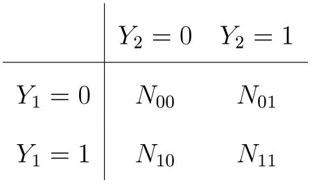(1)

with N₀₀ + N₀₁ + N₁₀ + N₁₁ = n. Correspondingly, we have the joint probability distribution

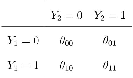with θ₀₀ + θ₀₁ + θ₁₀ + θ₁₁ = 1.0. We have θ₁ = P(Y₁ = 1) = θ₁₀ + θ₁₁ and θ₂ = P(Y₂ = 1) = θ₀₁ + θ₁₁; under H : θ₁ = θ₂, note θ₁₀ = θ₀₁. Call the common value of these off-diagonal probabilities θ_d when H is true. The subscript “d” denotes “dissimilarity”: θ_d = 0 denotes perfect agreement between Y₁ and Y₂; larger θ_d implies more mismatches.

Refer to (1), and let N_d = N₀₁ + N₁₀ denote the total number of observed “dissimilarities.” Under H, the conditional distribution of N₀₁ given N_d = n_d is the binomial distribution B(n_d, 0.5) (Mosteller, 1952). For observed values N₀₁ = n₀₁ and N_d = n_d, define the upper-tailed p-value for testing against the alternative θ₂ > θ₁ as

$$p\left(n_{01},n_d;\text{upper}\right)=P(B_{n_d,.5}\ge n_{01}),$$ (2)

where B_ν,p is a random variable distributed as binomial with parameters ν and p; similarly define p(n₀₁, n_d;lower) = P(B_nd,.5 ≤ n₀₁). The two-sided p-value is

$$p(n_{01},n_d;\text{two})=2min\{p(n_{01},n_d;\text{lower}),p(n_{01},n_d;\text{upper})\}.$$ (3)

The hypothesis H is rejected in favor of the appropriate alternative when p(n₀₁,n_d;*) ≤ α; type I error control is assured in all cases as follows.

Let P_H and E_H denote probability and expectation, respectively, when H is true. For the upper-tailed case, define

$$q(\alpha ,n_d;\text{upper})=P_H\{p(N_{01},N_d;\text{upper})\le \alpha \mid N_d=n_d\};$$

by construction, q(α, n_d;upper) ≤ α for all n_d = 0, 1,…,n. Hence the Type I error rate is

$$\begin{array}{ll}{P}_{\text{H}}(\text{Reject}H)& =P_H\{p(N_{01},N_d;\text{upper})\le \alpha \}\\ & =E_H\{q(\alpha ,N_d;\text{upper})\}\le \alpha .\end{array}$$ (4)

The argument for the lower tail and two-tailed cases is virtually identical; simply replace “upper” with either “lower” or “two.”

2.2 Asymptotic Versions

For large samples, a z-statistic may be used to test H. Define δ = θ₁ − θ₂, δ̂ = θ̂₁ − θ̂₂ = N₁₊/n − N₊₁/n and θ̂_ab = N_ab/n. Since Var(Y_i1−Y_i2) = (θ₀₁ + θ₁₀) − (θ₀₁ − θ₁₀)², a reasonable estimate of Var(δ̂) is $\widehat{\text{Var}}(\widehat{\delta })=\{({\widehat{\theta }}_{01}+{\widehat{\theta }}_{10})-{({\widehat{\theta }}_{01}-{\widehat{\theta }}_{10})}^2\}/n$, leading to

$$Z=\frac{\widehat{\delta }-\delta }{{\left\{\widehat{\mathit{\text{Var}}}(\widehat{\delta })\right\}}^{1/2}}\dot{\sim }N\left(0,1\right)$$ (5)

for large n, assuming that Var(Y_i1 − Y_i2) ≠ 0. Note that (5) is simply the paired-t statistic applied to the binary data pairs (Y_i1, Y_i2), using n rather than n − 1 for the denominator of the standard deviation estimate.

Under the null hypothesis H : θ₁ = θ₂ we have θ₁₀ = θ₀₁; hence under the null hypothesis an asymptotically equivalent version uses $\widehat{Va{r}_0}(\widehat{\delta })=({\widehat{\theta }}_{01}+{\widehat{\theta }}_{10})/n$ and either $\widehat{\mathit{\text{Var}}}(\widehat{\mathit{\delta }})$ or $\widehat{{\mathit{\text{Var}}}_0}(\widehat{\mathit{\delta }})$ could be used to normalize the test statistic. Using the $\widehat{{\mathit{\text{Var}}}_0}(\widehat{\mathit{\delta }})$ normalization,

$$Z_0=\frac{\widehat{\delta }-0}{{\left\{\widehat{Va{r}_0}(\widehat{\delta })\right\}}^{1/2}}\dot{\sim }N\left(0,1\right)$$ (6)

when δ = 0, again assuming that Var(Y_i1 − Y_i2) ≠ 0

For two-sided tests one may use the fact that $Z_0^2\dot{\sim }{\chi }_1^2$ under H; this manifestation is what is most commonly known by ‘McNemar's test,’ but we use (6) instead to allow one-sided tests. While (5) is not as commonly used, it is familiar as the paired-t statistic. It is also more convenient than (6) for the bootstrap analyses given in Section 7, since it provides the correct normalization when resampling from data that do not precisely obey the null hypothesis.

3 Multiple McNemar Tests

Suppose there are m hypotheses, each involving paired data with n_ℓ observations, ℓ = 1,…,m. For example, with trivariate binary data and all pairwise comparisons we have m = 3, with H₁ : θ₁ = θ₂, H₂ : θ₁ = θ₃, and H₃ : θ₂ = θ₃. As in Westfall and Troendle (2008), the proposed multiple comparisons method developed here is valid under very minimal assumptions. The main theorem of the paper requires the following assumption:

Assumption: Bivariate binary data pairs $\{y_{i1}^{\left(\ell \right)},y_{i2}^{\left(\ell \right)}\},i=1,\dots ,n_{\ell }$, are observable for pairs ℓ = 1,…,m.

Notice, we do not even assume any probability model at this point. Also, the data pairs may overlap: they may be pairs of columns of a multivariate binary matrix Y = {Y_ij}, i = 1,…, n; j = 1,…, p; or they may be disjoint, arising from distinct subgroups for example, thus the sample sizes n_ℓ are allowed to vary.

All probabilistic assumptions needed for the main theorem are embedded in the statements of the null hypotheses:

H_ℓ :The data pairs $\begin{array}{l}\{y_{i1,}^{\left(\ell \right)}{y}_{i2}^{\left(\ell \right)}\},i=1,\dots ,n_{\ell }\\ \end{array}$ are realizations of an i.i.d. bivariate Bernoulli process with ${\theta }_1^{\left(\ell \right)}={\theta }_2^{\left(\ell \right)}$.

As shown in Section 2.1, each H_ℓ can be tested using the exact McNemar test; the present goal is to test all m hypotheses with strong control of the FWER. We define the FWER to depend on a subgroup of true null hypotheses: suppose I = {ℓ₁,…,ℓ_m1} ⊆ {1,…,m} is the set of indexes of hypotheses that happen to be true (I is unknown in practice). Should I = Ø, there can be no type I errors, hence for the definition we assume I ≠ Ø:

$$\text{FWER}(I)=supP(\text{Reject}{H}_{\ell }\text{for some}\ell \in I).$$

Here “sup” refers to the supremum over all probability models for which the hypotheses in I are true. Strong control of the FWER at level α ∈ (0, 1) means that FWER(I) ≤ α no matter which set of null hypotheses indexed by I happens to be true (Hochberg and Tamhane, 1987). Weak control of the FWER means that FWER(I) ≤ α when I = {1,…,m}.

4 Testing Intersection Hypotheses

Since strong control of the FWER requires control for all subsets I, one typically must test intersection hypotheses of the form H_I = ∩_ℓ∈IH_ℓ to control the FWER. We use the “minP” test statistic

$$T_I({\mathit{\text{N}}}_I^{+})=\underset{\ell \in I}{min}{p}_{\ell }(N_{01}^{(\ell )},N_d^{(\ell )})$$

to test H_I, where $p_{\ell }(N_{01}^{(\ell )},N_d^{(\ell )})$ is the p-value for $H_{\ell }:{\theta }_1^{(\ell )}={\theta }_2^{(\ell )}$ and ${\mathit{\text{N}}}_I^{+}=\{N_{01}^{(\ell )},N_d^{(\ell )}\mid \ell \in I\}$. Sidedness is understood from the subscript ℓ on p that indicates the researcher's choice for that particular comparison, and the indices “upper,” “lower” and “two” in (2) and (3) will henceforth be dropped.

Letting ${\mathit{\text{N}}}_I=\{N_d^{(\ell )}\mid \ell \in I\}$ and n_I denote an observed value of N_I, define the critical value as

$$c_I^{\alpha }({\mathit{\text{n}}}_I)=\text{max}\left[c:\sum _{\ell \in I}{P}_{H_{\ell }}\left\{p_{\ell }(N_{01}^{(\ell )},N_d^{(\ell )})\le c\mid N_d^{(\ell )}=n_d^{(\ell )}\right\}\le \alpha \right]$$ (7)

if such a c exists, and let $c_I^{\alpha }({\mathit{\text{n}}}_I)=0$ otherwise.

Theorem 1 The test that rejects H_I when $T_I({\mathit{\text{N}}}_I^{+})\le c_I^{\alpha }({\mathit{\text{N}}}_I)$ has type I error rate ≤ α.

The proof is given online at www.biometrics.tibs.org.

It is convenient to express rejection rules using p-values rather than fixed α-level rejection rules. The rejection rule $T_I({\mathit{\text{n}}}_I^{+})\le c_I^{\alpha }({\mathit{\text{n}}}_I)$ is equivalently stated as ${\stackrel{\sim }{p}}_I({\mathit{\text{n}}}_I^{+})\le \alpha$ where

$${\stackrel{\sim }{p}}_I({\mathit{\text{n}}}_I^{+})=\sum _{\ell \in I}{P}_{H_{\ell }}\left\{p_{\ell }(N_{01}^{(\ell )},N_d^{(\ell )})\le T_I({\mathit{\text{n}}}_I^{+})\mid N_d^{(\ell )}=n_d^{(\ell )}\right\}.$$ (8)

Expression (8) shows most clearly why the discrete method offers power gains. If the conditional distributions of p-values $p_{\ell }(N_{01}^{(\ell )},N_d^{(\ell )})$ were uniform, then we would have

$$P_{H_{\ell }}\left\{p_{\ell }(N_{01}^{(\ell )},N_d^{(\ell )})\le T_I({\mathit{\text{n}}}_I^{+})\mid N_d^{(\ell )}=n_d^{(\ell )}\right\}=T_I({\mathit{\text{n}}}_I^{+}),$$

and (8) would reduce to ${\stackrel{\sim }{p}}_I({\mathit{\text{n}}}_I^{+})=|H_I|\times T_I({\mathit{\text{n}}}_I^{+})$, the Bonferroni test statistic. However, as noted in Section 2.1, $P_{H_{\ell }}\left\{p_{\ell }(N_{01}^{(\ell )},N_d^{(\ell )})\le T_I({\mathit{\text{n}}}_I^{+})\mid N_d^{(\ell )}=n_d^{(\ell )}\right\}\le T_I({\mathit{\text{n}}}_I^{+})$ by construction. In fact, for small $n_d^{(\ell )}$ the support of the binomial distribution extends little into the tails and we have

$$P_{H_{\ell }}\left\{p_{\ell }(N_{01}^{(\ell )},N_d^{(\ell )})\le T_I({\mathit{\text{n}}}_I^{+})\mid N_d^{(\ell )}=n_d^{(\ell )}\right\}=0;$$

for example, $P(P_{\ell }\le .05\mid N_d^{(\ell )}=n_d^{(\ell )})=0$ when $n_d^{(\ell )}\le 5$ and P_ℓ is the two-sided McNemar p-value. Discreteness of the binomial distributions may imply

$$P_{H_{\ell }}\left\{p_{\ell }(N_{01}^{(\ell )},N_d^{(\ell )})\le T_I({\mathit{\text{n}}}_I^{+})\mid N_d^{(\ell )}=n_d^{(\ell )}\right\}\ll T_I({\mathit{\text{n}}}_I^{+})$$

for other ℓ The end result is that in cases of small to moderate sample sizes (implying small $n_d^{(\ell )}$), we can have ${\stackrel{\sim }{p}}_I({\mathit{\text{n}}}_I^{+})\ll |H_I|\times T_I({\mathit{\text{n}}}_I^{+})$, i.e., a dramatic improvement over the Bonferroni test. High correlation between variables also produces sparseness as $n_d^{(\ell )}$ is inversely related to correlation; hence, even though the method uses the Boole inequality and thus does not incorporate correlation directly, its power can still be high due to high binary correlations.

5 The Bonferroni-Holm Method

Holm (1979) introduced a step-down procedure to control the FWER with uniform improvement over the classic Bonferroni method. Letting p₍₁₎ ≤ … ≤ p_(m) denote ordered p-values corresponding to hypotheses H₍₁₎, …, H_(m), the method rejects all H_(j) where max_ℓ≤j{(k − ℓ + 1)p_(ℓ)} ≤ α. Equivalently, defining the Bonferroni-Holm adjusted p-value as ${\stackrel{\sim }{p}}_{(j)}^{BH}=min(1,{max}_{\ell \le j}\{(k-\ell +1)p_{(\ell )}\})$, the method rejects all H_(j) where ${\stackrel{\sim }{p}}_{(j)}^{BH}\le \alpha$. Assuming that the unadjusted p-values are uniformly distributed or stochastically larger than uniform so that P(P_ℓ ≤ α) ≤ α, all α ∈ (0, 1), Holm proved FWER control in the strong sense.

As shown in (4), the exact McNemar p-value satisfies the stochastic uniformity condition, hence Holm's method applied to the exact McNemar p-values has strong control of the FWER. However, the classical McNemar test (6) does not satisfy stochastic uniformity (Berger and Sidik, 2003), hence FWER control when using Holm's method applied to (6) can be stated only approximately.

6 The Discrete Bonferroni-Holm Method for Exact McNemar Tests

As described after (8), use of discrete distributions can dramatically improve the power of joint tests. The discrete multiple testing method proceeds by testing successive subset intersection hypotheses in the order of the observed p-values. For exact McNemar p-values (using (2), (3), or the lower-tail version), define p_(j) = p_rj, so that r₁,…,r_m are the indexes of the p-values sorted from smallest to largest. When there are ties, the indexes may be chosen in arbitrary order. Define nested index sets R_ℓ = {r_ℓ,…,r_m},ℓ = 1,…,m and consider the p-values ${\stackrel{\sim }{p}}_{R_{\ell }}({\mathit{\text{N}}}_{R_{\ell }}^{+})$ defined in (8) for testing these subsets. The discrete Bonferroni method proceeds by sequentially testing the subset hypotheses H_Rℓ as shown in Section 4, stopping as soon as a hypothesis is not rejected. Specifically, defining the adjusted p-value for H_(j) as ${\stackrel{\sim }{p}}_{(j)}={max}_{\ell \le j}\{{\stackrel{\sim }{p}}_{R_{\ell }}(N_{R_{\ell }}^{+})\}$, the discrete Bonferroni method rejects all H_(j) where p̃_(j) ≤ α. That the method controls the FWER in the strong sense is proven in the following theorem whose proof is given online at www.biometrics.tibs.org.

Theorem 2 If the assumption and null hypotheses are as given in Section 3, then the discrete Bonferroni method controls the FWER in the strong sense.

7 Incorporating Dependence Using the Bootstrap

The discrete method may be criticized for relying on the Boole inequality and thus not accounting for dependence structure among the tests. Klingenberg and Agresti (2006) describe a special multivariate structure where the variables fall into two groups, in which case one can randomly permute groups within a row, independently for all rows. Extending their method to the general case described here, one might permute all observations within a row, but this approach would destroy the correlation structure, enforce an artificial complete null hypothesis, and be incompatible with the marginal McNemar tests in that the number of dissimilarities N_d for a given column would not be fixed for all permutation samples. Instead, we develop a bootstrap approach. We lose the generality of the discrete method, restricting our attention to pairwise comparisons of proportions from i.i.d. multivariate Bernoulli data. Specifically, we assume

$$\mathit{\text{Y}}=\left[\begin{array}{c}{\mathit{\text{Y}}}_1^{\prime }\\ ⋮\\ {\mathit{\text{Y}}}_n^{\prime }\end{array}\right]$$

where the ${\mathit{\text{Y}}}_i^{\prime }=[Y_{i1}\dots Y_{ig}]$ are i.i.d. multivariate Bernoulli, with $E({\mathit{\text{Y}}}_i^{\prime })=[{\theta }_1\dots {\theta }_{\mathrm{g}}]$. Null hypotheses are H_ℓ : θ_aℓ = θ_bℓ, for a set of index pairs (a_ℓ, b_ℓ), ℓ = 1,…,m. Commonly considered sets of pairs are all pairwise comparisons of proportions (m = g(g − 1)/2), and comparisons against a common proportion (m = g − 1).

The method uses paired differences. Construct the derived variables D_iℓ = Y_iaℓ − Y_ibℓ, the collated vectors ${\mathit{\text{D}}}_i^{\prime }=[D_{i1}\dots D_{im}]$ and the data matrix

$$\mathit{\text{D}}=\left[\begin{array}{c}{\mathit{\text{D}}}_1^{\prime }\\ ⋮\\ {\mathit{\text{D}}}_n^{\prime }\end{array}\right].$$

Note that the rows of D are i.i.d. with $E({\mathit{\text{D}}}_i^{\prime })=\mathit{\delta }\prime =[{\delta }_1\dots {\delta }_m]$

Let D̅) = [D̅₁ … D̅_m]′ with D̅_ℓ Σ_ℓ D_iℓ/n, and let $\mathit{\text{S}}=\mathit{\text{diag}}\{{\mathit{\text{s}}}_{\mathit{\ell }}^2\}$ with $s_{\ell }^2={\sum }_{\ell }{(D_{i\ell }-{\overline{D}}_{\ell })}^2/n)$. Provided Var(D_iℓ) > 0 for all ℓ, standard asymptotic theory yields that

$$\mathit{\text{Z}}=n^{1/2}{\mathit{\text{S}}}^{-1/2}(\overline{\mathit{\text{D}}}-\mathit{\delta })$$

converges in distribution to a (possibly singular) multivariate normal distribution with mean vector 0 and covariance matrix Ω whose diagonal elements are 1. Individual elements of Z are the Z-statistics in (5).

The main results shown in Sections 4 and 6 of this paper provides rigorous theory for exact tests in finite samples. Rigorous asymptotic theory surrounding the various versions of the approximate McNemar test are straightforward and are found elsewhere; rigorous asymptotic theory concerning the bootstrap multiple testing methods to be described can also be found elsewhere in closely related contexts (e.g., Bickel and Freedman, 1981; Romano and Wolfe, 2005).

Let

$${\mathit{\text{D}}}^{\ast }=\left[\begin{array}{c}{\mathit{\text{D}}}_1^{\ast \prime }\\ ⋮\\ {\mathit{\text{D}}}_n^{\ast \prime }\end{array}\right]$$

be obtained by sampling the rows of D with replacement; this is a bootstrap sample. Identify corresponding summary statistics D̅* and S*. Standard bootstrap asymptotic theory holds that the distribution of Z* = n^1/2S*^−1/2(D̅* − D̅) also converges to N(0, Ω) (e.g., Theorem 2.2 of Bickel and Freedman, 1981).

Consider an intersection hypothesis H_I and let Z_I = {Z_ℓ; ℓ ∈ I}, where Z_ℓ is obtained as in (5) but setting δ_ℓ = 0. If H_I is true, then Z_I converges in distribution to N(0, Ω_I), where Ω_I denotes a covariance matrix that is constrained by H_I but is otherwise arbitrary; by standard bootstrap theory ${\mathit{\text{Z}}}_I^{\ast }=\{Z_{\ell }^{\ast };\ell \in I\}$ also converges to N(0, Ω_I) when H_I is true. Supposing the test statistic is $Z_I^{(max)}={max}_{\ell \in I}\{|Z_{\ell }|\}$ (modifications for upper-tailed, lower tailed or mixed tests are straightforward but clutter the notation), the null distribution of $Z_I^{(max)}$ is asymptotically the same as that of $Z_I^{\ast (max)}={max}_{\ell \in I}\{|Z_{\ell }^{\ast }|\}$. Hence an approximately valid bootstrap p-value for testing H_I is

$$p_I^{\ast }=P^{\ast }(Z_I^{\ast (max)}\ge z_I^{(max)}).$$

Using these bootstrap p-values to test intersection null hypotheses, the step-down algorithm based on testing intersection hypotheses in the order of the observed test statistics z₍₁₎ ≥ …≥ z_(m) as described in Section 6 is used. Approximate FWER control can be established loosely as in the proof of Theorem 2; however, FWER control is not guaranteed. On the other hand, the method might be more powerful since it incorporates dependence structures, both those inherent among the original binary variables Y, and also those that are manufactured through the pairwise contrasts.

A difficulty caused by discreteness is seen in the definition of the Z-statistics. In cases where the standard of deviation of {D_iℓ} is 0, both Z_ℓ and $Z_{\ell }^{\ast }$ are undefined. In most testing applications, this will happen when D_iℓ = 0 or $D_{i\ell }^{\ast }=0$, all i = 1,…,n; it would be highly unusual for this to occur in practice with either D_iℓ ≡ 1, D_iℓ ≡ −1, $D_{i\ell }^{\ast }\equiv 1$, or $D_{i\ell }^{\ast }\equiv -1$. Hence in the case where any standard deviation (raw or bootstrapped) is zero, the corresponding Z-statistic is also assigned to zero.

8 Applications

8.1 Multiple Classification Models

Data mining and machine learning algorithms produce many complex classification models. Deciding on the best model is typically done using out-of-sample prediction accuracy; heretofore, rigorous methods are lacking for performing multiple comparisons among the models. When the true state is binary (e.g., existence of cancer) and the model provides a similar Yes/No prediction, prediction accuracy can be measured by binary matches where (model prediction) = (true state). Typically these matches are separated into positive and negative true states; the proportion of matches is called sensitivity and specificity respectively.

Multiple comparisons problems arise when comparing sensitivity, specificity, and overall accuracy among several models. For example, if there are 5 models, there are 10 pairwise model comparisons, and 10 (comparisons) ×3 (accuracy measures)= 30 total tests. The dependence structure among this collection of tests is complex and there are intricate logical dependencies among the sensitivity, specificity, and global tests, as well as among the multiple pairwise comparisons. Developing a bootstrap model to incorporate all such complexities can be done, but with difficulty, and without guarantee of FWER control. The discrete Bonferroni method with McNemar's exact test mathematically controls the FWER in this case as in many other cases and, as we will see, has reasonable power.

In the Microarray Quality Control Phase II Project (MAQC-II, Shi et al., 2009), a goal is evaluate classifiers that use microarray data. Using six training datasets, 36 data analysis groups developed more than 18,000 gene-expression based models to predict 3 toxicological and 10 clinical endpoints. The models were then applied to six independent and blinded validation datasets to evaluate their performance at predicting the endpoints. A subset of the data is used for the purposes of comparisons here; the particular endpoint used is Multiple Myeloma two-year survival (MM), and the 20 models developed by the group at Cornell university are studied. The data set is available from the authors.

The validation data set has (n = 214) study patients, 27 of whom have MM; the indicator variable T = 0, 1 denotes absence or presence. Model predictions are T̂ = 0, 1, and correct classification is determined as Y = 1 −|T − T̂|. The overall correct classification estimate is Σ_iY_i/n, while the sensitivity and specificity estimates are Σ_iY_i1_Ti=1/Σ_i1_Ti=1 and Σ_iY_i1_Ti=0/Σ_i1_Ti=0 respectively, where 1_A is the indicator of the event A. There are 20 models, leading to 20 × 19/2 = 190 pairwise model comparisons for each of the three measures, and there are 3 × 190 = 570 comparisons total. Table 1 summarizes the results for the most significant of the 570 comparisons among accuracy measures.

Table 1.

Multiple testing using two-sided p-values for multiple models and performance measures. Comparison denotes models and measure; e.g., “12-16, all” compares models 12 and 16 with respect to the overall accuracy. “Ex” refers to exact p-values calculated from (3), “McN” refers to the McNemar test based on (6), Disc” refers to the discrete multiplicity adjustment, and “Holm” refers to the usual Bonferroni-Holm adjustment.

Comparison	${\widehat{\theta }}_1^{(\ell )}$	${\widehat{\theta }}_2^{(\ell )}$	pℓ,Ex	pℓ,McN	${\stackrel{\sim }{p}}_{\ell ,\text{Ex}}^{\text{Disc}}$	${\stackrel{\sim }{p}}_{\ell ,\text{Ex}}^{\text{Holm}}$	${\stackrel{\sim }{p}}_{\ell ,\text{McN}}^{\text{Holm}}$
12-16, all	.832	.893	.00024	.00031	.0042	.1392	.1776
12-20, all	.832	.893	.00098	.00079	.0396	.5557	.4490
6-17, spec	.941	1.00	.00098	.00091	.0396	.5557	.5175
6-15, spec	.941	1.00	.00098	.00091	.0396	.5557	.5175
6-20, spec	.941	1.00	.00098	.00091	.0396	.5557	.5175
9-16, all	.841	.893	.00098	.00091	.0396	.5557	.5175
2-6, spec	.995	.941	.00195	.00157	.0757	1.00	.8829
(563 more)	⋮	⋮	⋮	⋮	⋮	⋮	⋮

Even though the “Exact” unadjusted p-values are larger than the McNemar asymptotic p-values, the discrete method of multiplicity adjustment produces far smaller adjusted p-values, showing 6 statistically significant differences at the nominal FWER = .05 level.

8.2 Comparing Adverse Event Rates

Comparing adverse event (AE) rates for single-sample multivariate binary data is of interest in crossover trials (Klingenberg and Agresti, 2006), where the same AEs are compared for different treatments, as well as in Phase IV clinical trials, where significantly aberrant AEs are flagged for further attention. Consider the adverse event data set provided by Westfall et al. (1999, p. 243). There are two groups, control and treatment, with 80 patients in each group, 28 adverse events reported, the last of which is an indicator of any adverse event and is excluded from our analysis. To mimic a Phase IV study, we restrict our attention to the treatment patients, and compare the adverse event rates among the 27 × 26/2 = 351 pairwise combinations, all tested using McNemar tests and adjusted for multiplicity as shown above. Table 2 displays the partial results.

Table 2.

Multiple testing using two-sided p-values for all pairwise comparisons of adverse events. Comparison denotes adverse event rates that are compared; e.g., “1-(12 others)” shows data comparing adverse event labeled 1 with 12 other adverse events. The entries are the same for all 12 because the counts are identical, and are listed in a single row rather than 12 rows to save space. Refer to Table 1 legend for remaining terminology. The final column refers to unadjusted p-values computed using (5) and multiplicity-adjusted using the bootstrap to accommodate dependence structure.

Comparison	${\widehat{\theta }}_1^{(\ell )}$	${\widehat{\theta }}_2^{(\ell )}$	pℓ,Exact	pℓ,McN	${\stackrel{\sim }{p}}_{\ell ,\text{Ex}}^{\text{Disc}}$	${\stackrel{\sim }{p}}_{\ell ,\text{Ex}}^{\text{Holm}}$	${\stackrel{\sim }{p}}_{\ell ,\text{McN}}^{\text{Holm}}$	${\stackrel{\sim }{p}}_{\ell ,}^{\text{Boot}}$(5)
1-(12 others)	.313	.000	0+	0+	0+	0+	.0002	.0035
(11 more)	⋮	⋮	⋮	⋮	⋮	⋮	⋮	⋮
1-8	.313	.063	.00009	.00009	.0002	.0289	.0288	.0250
1-3	.313	.075	.00016	.0001	.0002	.0512	.0473	.0334
1-2	.313	.100	.00151	.00107	.0037	.4935	.3486	.1219
2-11	.100	.000	.00781	.00486	.2105	1.00	1.00	.3155
(324 more)	⋮	⋮	⋮	⋮	⋮	⋮	⋮	⋮

Again, the discrete method shows better results, despite using exact McNemar tests for which the unadjusted p-values tend to be larger than for the approximate McNemar tests. In particular, the method shows adverse event labeled 1 as different from all others; the Holm method misses the 1-2 difference when used with the approximate McNemar test, and it misses both the 1-2 and the 1-3 differences when used with the exact McNemar test.

The last column in Table 2 shows the results of the bootstrap method. The discrete method using exact tests clearly outperforms the bootstrap in this example, despite the fact that the unadjusted p-values for the exact tests are larger, and despite the fact that the bootstrap method incorporates dependence structure and the discrete method with exact tests does not. On the other hand, comparing the last two columns ( ${\stackrel{\sim }{p}}_{\ell ,\text{McN}}^{\text{Holm}}$ and ${\stackrel{\sim }{p}}_{\ell ,(5)}^{\text{Boot}}$) of the bottom four rows shows that incorporating dependence structure reduces the adjusted p-values, as expected. (The top rows are an exception due to unusual behavior in the extreme tails of the distribution of the max Z* statistic.)

9 Simulation Study

In this section we compare the various procedures described above in the case of comparisons against a “control” proportion, when there are g = 11 multivariate binary proportions (hence there are m = 10 pairwise comparisons). We assume a multivariate probit threshold model with either (i) fixed compound symmetric covariance matrix, (ii) random covariance matrix with positive entries that follow the one-factor factor analysis model, or (iii) a random covariance matrix model with both positive and negative entries that follow the single-factor factor analysis model.

Specifically, we generate X_i∼_iid N_g(μ,Φ), and define Y_ij = l_xij<0. The parameter vector μ is chosen to reflect either large probabilities (near .5) or small probabilities (near 0). In all cases Φ has unit diagonals. In covariance model (i), the off-diagonals are specified as ρ, a fixed constant, called the “CS” model. In models (ii) and (iii), we generate Φ at random via Σ = ηη′ + σ²I, where η is a row vector of i.i.d. random variables and σ² is a given constant, then normalize to obtain Φ = (diagΣ)^−1/2Σ(diagΣ)^−1/2. For case (ii), the random variables are generated as U(0, 1) (called the FA⁺ model), and for case (iii) they are generated as U(−1, 1) (called the FA^+/− model). In both (ii) and (iii), the off-diagonal squared correlations are random with ${\rho }^2={\eta }_i^2{\eta }_j^2/\{({\eta }_i^2+{\sigma }^2)({\eta }_j^2+{\sigma }^2)\}$; hence $E({\rho }^2)={[E\{{\eta }_i^2/({\eta }_i^2+{\sigma }^2)\}]}^2={\{1-\sigma {tan}^{-1}(1/\sigma )\}}^2$. Setting σ = 0.033378, 0.21561 makes E(ρ²) = 0.9, 0.5; these values are used in the simulation study.

FWER is estimated as the proportion of simulations where any type I error occurs. Power can be estimated as the proportion of simulations (i) where any non-null difference is discovered, (ii) where all non-null differences are discovered, and (iii) as the average proportion of non-null differences that are discovered. In the interest of space we use only (iii). The nominal FWER is set to 0.05, the number of simulations is 10,000, and the number of bootstrap samples is 999 for all cases shown in Table 3.

Table 3.

Power comparison of the procedures, n = 100.

			Power
μ′	Covariance	E(ρ2)	Disc, Ex	Holm, Ex	Holm, McN	Boot, (5)
[0×10, .4]	any	0	.26	.23	.26	.30
[0×10, .4]	CS	.5	.59	.52	.58	.64
[0×10, .4]	FA+	.5	.63	.57	.62	.66
[0×10, .4]	FA+/−	.5	.80	.74	.78	.80
[0×10, .4]	CS	.9	.96	.92	.95	.94
[0×10, .4]	FA+	.9	.94	.90	.92	.94
[0×10, .4]	FA+/−	.9	.97	.95	.96	.97
[−1.96×10, −1.28]	any	0	.40	.17	.24	.23
[−1.96×10, −1.28]	CS	.5	.60	.26	.36	.41
[−1.96×10, −1.28]	FA+	.5	.59	.26	.36	.44
[−1.96×10, −1.28]	FA+/−	.5	.69	.30	.43	.57
[−1.96×10, −1.28]	CS	.9	.77	.34	.48	.72
[−1.96×10, −1.28]	FA+	.9	.75	.33	.47	.71
[−1.96×10, −1.28]	FA+/−	.9	.75	.33	.47	.74

Additional simulations are provided in the web on-line content, including different sample sizes, and the case of all pairwise comparisons.

Notes on the simulations, including those from the web on-line content:

• Higher correlations generally make tests more powerful because they increase the precision of the estimated difference as noted by Agresti (2002, p. 412).

• Lack of power of the exact McNemar test relative to the approximate version is shown in the comparison of the “Holm, Ex” columns with the “Holm, McN” columns.

• Despite lack of power of the exact McNemar test relative to the approximate version, the use of the exact McNemar test with the discrete Bonferroni-Holm adjustments (the “Disc, Ex” columns) had higher estimated power than the approximate McNemar test with Bonferroni-Holm adjustment in all cases considered.

• There is no clear winner when comparing the step-down bootstrap adjustments (the “Boot, (5)” columns) with the discrete Bonferroni-Holm adjustments. The power differences can be large favoring either method.

• The “CS” covariance structure is most uniform in the correlations, the FA^+/− is least uniform, and FA⁺ is intermediate. The bootstrap fares relatively better when the correlations are less uniform.

• FWER control is mathematically proven for the discrete method using exact tests, and the Holm method when applied to the exact tests as shown above in Theorem 2. In all cases of the simulations, the estimated FWER levels were usually well below .05 for these tests and are not shown. However, on occasions the bootstrap method exceeded the nominal FWER=.05 level. For example, in the cases indicated by the bottom three rows of Table 3, the estimates of FWER for the bootstrap method were .053, .068, and .070, respectively The complete null configuration (μ_i ≡ −1.96, i = 1,…, 11) fares even worse for the bootstrap in these cases, with estimated FWERs .068, .089, and .091. These six estimates are each based on 100,000 simulations of 9,999 bootstrap samples, so the excesses are real. Particularly intriguing is the fact that the bootstrap method both exceeds the nominal FWER and is less powerful for these cases.

10 Conclusion

We have developed stepwise multiple testing methods for dependent proportions that account for discreteness and correlation structures. Analytical and simulation results suggest using either the exact McNemar test with the discrete Bonferroni-Holm multiplicity adjustment or the bootstrapped step-down procedure using the statistics (5) as base tests. Bonferroni-Holm with the ordinary McNemar (large sample) test and with the exact McNemar p-values are inferior methods.

Favoring the bootstrapped statistic (5) is the fact that it accounts for correlation structure, which often improves power, in some cases dramatically. In addition, the discrete method is asymptotically conservative since it does not account for correlation structures, while the bootstrap method is asymptotically consistent. Thus the bootstrap is preferred in applications with large sample sizes.

On the other hand, we found occasional cases of excess Type I errors for the bootstrap procedure in our simulations; see also Klingenberg et al. (2008). Troendle, Korn and McShane (2004) note that the asymptotic convergence needed for successful application of the bootstrap can be very slow in high dimensional multiple testing applications, also leading to excess type I error rates for bootstrap multiple testing applications.

Favoring the discrete method is that it mathematically controls the FWER in finite samples; one need not simulate to assess FWER control as is needed with the bootstrap or other approximate methods. Also, the discrete method can be used under minimal assumptions on the data structure, and one need not develop specific algorithms for every situation (see Table 1 for an example of a non-standard application). Further, the finite-sample power of the method in some cases is higher than that of the bootstrap procedure. Finally, there are uncomfortable, ad hoc assignments that must be made using the bootstrap, such as how to assign the value of the test statistic when the standard deviation is zero. There are also clear signs with discrete data that the asymptotic plateau has not been reached, such as the case where a column of the data set is all 0's. In this case, the bootstrap population probability is 0, which is clearly wrong. Such ad hoc assignments and lack of asymptotic validity in small samples are of no concern when using the discrete method with exact tests.

References

- Agresti A. Categorical Data Analysis. New York: John Wiley and Sons; 2002. [Google Scholar]
- Berger RL, Sidik K. Exact unconditional tests for a 2×2 matched-pairs design. Statistical Methods in Medical Research. 2003;12:91–108. doi: 10.1191/0962280203sm312ra. [DOI] [PubMed] [Google Scholar]
- Bhakpar VP, Somes GW. Multiple comparisons of matched proportions. (A).Communications in Statistics. 1976;7:17–25. [Google Scholar]
- Bickel PJ, Freedman DA. Some asymptotic theory for the bootstrap. The Annals of Statistics. 1981;9:1196–1217. [Google Scholar]
- Demšar J. Statistical comparisons of classifiers over multiple data sets. Journal of Machine Learning Research. 2006;7:1–30. [Google Scholar]
- Durkalski VL, Palesch YY, Lipsitz SR, Philip F, Rust PF. The analysis of clustered matched-pair data. Statistics in Medicine. 2003;22:2417–2428. doi: 10.1002/sim.1438. [DOI] [PubMed] [Google Scholar]
- Hochberg Y, Tamhane A. Multiple Comparisons Procedures. New York: John Wiley and Sons; 1987. [Google Scholar]
- Holm S. A simple sequentially rejective multiple test procedure. Scandinavian Journal of Statistics. 1979;6:65–70. [Google Scholar]
- Kitajima K, Murakami K, Yamasaki E, Domeki Y, Kaji Y, Morita S, Suganuma N, Sugimura K. Performance of integrated FDG-PET/contrast-enhanced CT in the diagnosis of recurrent uterine cancer: Comparison with PET and enhanced CT. European Journal of Nuclear Medicine and Molecular Imaging. 2009;36:362–372. doi: 10.1007/s00259-008-0956-1. [DOI] [PubMed] [Google Scholar]
- Klingenberg B, Agresti A. Multivariate extensions of McNemar's test. Biometrics. 2006;62:921–928. doi: 10.1111/j.1541-0420.2006.00525.x. [DOI] [PubMed] [Google Scholar]
- Klingenberg B, Solari A, Salmaso L, Pesarin F. Testing marginal homogeneity against stochastic order in multivariate ordinal data. Biometrics. 2009;65:452–462. doi: 10.1111/j.1541-0420.2008.01067.x. [DOI] [PubMed] [Google Scholar]
- Leisenring W, Alonzo T, Pepe MS. Comparisons of predictive values of binary medical diagnostic tests for paired designs. Biometrics. 2000;56:345–351. doi: 10.1111/j.0006-341x.2000.00345.x. [DOI] [PubMed] [Google Scholar]
- Lyles RH, Williamson JM, Lin HM, Heilig CM. Extending McNemar's test: Estimation and inference when paired binary outcome data are misclassified. Biometrics. 2005;61:287–294. doi: 10.1111/j.0006-341X.2005.040135.x. [DOI] [PubMed] [Google Scholar]
- Mosteller F. Some statistical problems in measuring the subjective response to drugs. Biometrics. 1952;8:220–226. [Google Scholar]
- Rabinowitz D, Betensky RA. Approximating the distribution of maximally selected McNemar's statistics. Biometrics. 2000;56:897–902. doi: 10.1111/j.0006-341x.2000.00897.x. [DOI] [PubMed] [Google Scholar]
- Romano JP, Wolfe M. Exact and approximate stepdown methods for multiple hypothesis testing. Journal of the American Statistical Association. 2005;100:94–108. [Google Scholar]
- Shi L, et al. The MAQC-II project: A comprehensive study of common practices for the development and validation of microarray-based predictive models. Nature Biotechnology. 2009 doi: 10.1038/nbt.1665. 193 others. Submitted. [DOI] [PMC free article] [PubMed] [Google Scholar]
- Troendle JF, Korn EL, McShane LM. An example of slow convergence of the bootstrap in high dimensions. The American Statistician. 2004;58:25–29. [Google Scholar]
- Westfall PH, Tobias R, Rom D, Wolfinger R, Hochberg Y. Multiple Comparisons and Multiple Tests using SAS®. SAS®Institute; Cary, NC: 1999. [Google Scholar]
- Westfall PH, Troendle JF. Multiple testing with minimal assumptions. Biometrical Journal. 2008;50:745–755. doi: 10.1002/bimj.200710456. [DOI] [PMC free article] [PubMed] [Google Scholar]