A 3-D constrained mixture model for mechanically mediated vascular growth and remodeling

Abstract

In contrast to the widely applied approach to model soft tissue remodeling employing the concept of volumetric growth, microstructurally motivated models are capable of capturing many of the underlying mechanisms of growth and remodeling; i.e., the production, removal, and remodeling of individual constituents at different rates and to different extents. A 3-dimensional constrained mixture computational framework has been developed for vascular growth and remodeling, considering new, microstructurally motivated kinematics and constitutive equations and new stress and muscle activation mediated evolution equations. Our computational results for alterations in flow and pressure, using reasonable physiological values for rates of constituent growth and turnover, concur with findings in the literature. For example, for flow-induced remodeling, our simulations predict that, although the wall shear stress is restored completely, the circumferential stress is not restored employing realistic physiological rate parameters. Also, our simulations predict different levels of thickening on inner versus outer wall locations, as shown in numerous reports of pressure-induced remodeling. Whereas the simulations are meant to be illustrative, they serve to highlight the experimental data currently lacking to fully quantify mechanically mediated adaptations in the vasculature.

1 Introduction

Vascular remodeling plays a key role in many physiological and pathophysiological processes, as well as the success (or failure) of many clinical interventions; examples include vascular development and aging, hypertension and atherosclerosis, and restenosis of vascular grafts. Despite the explosion of information on vascular remodeling, from the molecular level to the tissue level, there remains a pressing need to integrate these data into a predictive multiscale model. Humphrey and Rajagopal said that in order to capture the salient features of these remodeling processes ‘one must track local balances or imbalances in the continual production, removal, [and remodeling] of individual constituents, the mechanical state in which the constituents are formed, and how these constituents are organized (Humphrey and Rajagopal 2002). Abdominal aortic aneurysms (AAA’s) provide a good illustration of the need for a multiscaled microstructurally motivated mathematical model. During progression of AAA’s, circumferential expansion, vessel wall thinning, and axial lengthening are coincident with a progressive loss of elastin and smooth muscle and decrease in glycosaminoglycans, with mature aneurysms consisting primarily of collagen and fibroblasts; thus, AAA’s experience spatial and temporal variations in their geometry, microstructural content and organization, and applied loads. To develop a predictive model for vascular remodeling, the complex interplay between evolving material behavior, geometry, and applied loads (which together determine the local mechanical environment) and the mechanobiological response to this changing mechanical environment must be incorporated.

In contrast to the widely applied approach of modeling soft tissue remodeling using the concept of volumetric growth, put forth by Skalak (Skalak 1981; Skalak et al. 1996) and extended by many (Fridez et al. 2001; Rachev 2000; Raykin et al. 2009; Rodriguez et al. 1994; Taber 1998; Taber and Eggers 1996; Taber et al. 1995), several groups have taken modeling approaches that can be categorized as microstructurally motivated models (Humphrey and Rajagopal 2002; Barocas and Tranquillo 1997a,b; Driessen et al. 2003a,b, 2004a, b, 2005; Kuhl et al. 2005; Gleason and Humphrey 2004, 2005a; Gleason et al. 2004a; Humphrey and Rajagopal 2003; Mow et al. 1980). Whereas a true microstructural model of native tissues requires one to include the highly complex protein interactions at many hierarchical length scales (e.g., organization of collagen from tropocollagen, to a microfibril, to a subfibril, to a fibril, to higher order tissue structures (Baer et al. 1992) and may be decades away, microstructurally motivated (yet phenomenological) models will continue to provide insights that guide experiments and help one to interpret experimental results. The commonality of all of these microstructurally motivated models is that the underlying constitutive behavior includes information at the microstructural level, and the remodeling of the tissue is quantified by quantifying changes at this scale (in contrast to the volumetric approach that quantifies changes at the whole tissue level). The key differences between each microstructural approach is the wide variety of theoretical frameworks and constitutive and evolution equations employed.

Here we employ the general theoretical framework described by Humphrey and Rajagopal (2002) for soft tissue growth and remodeling. The purpose of this paper is to develop a computational framework for vascular remodeling that is capable of quantifying spatial and temporal changes in the local mechanical response function in terms of microstructurally motivated metrics. We extend our (2-dimensional) framework for blood vessel remodeling to altered mechanical loading (Gleason and Humphrey 2004, 2005a,b; Gleason et al. 2004a,b) to a 3-dimensional framework and consider new, microstructurally motivated kinematics and constitutive equations and new evolution equations which relate constituent growth, turnover, and remodeling to stress and muscle activation. Our model is capable of capturing growth and remodeling in response to individual or combined alterations in flow, pressure, and axial stretch, based on reasonable physiological values for rates of constituent growth and turnover. Our modeling framework and illustrative simulations can be used to motivate experimental design to identify the most insightful experiments to be performed and to better understand vascular growth and remodeling.

2 Theoretical framework

2.1 Kinematics

Given the need to track the production and removal of individual constituents, as well as the mechanical states in which these constituents are formed, we model the artery as a constrained mixture. Consider a local neighborhood about a point with position x(r, θ, z) in the loaded configuration; let this neighborhood κ_t be defined as a cylindrical sector with sides of length rdθ, dz, and dr (Fig. 1a). Let this neighborhood be denoted κ_n in the locally stress-free (or natural) configuration for the mixture, which has position X(R, Θ, Z); let this sector have sides RdΘ, dZ, and dR. Since constituents are constrained to deform together, the current position of each constituent j, denoted x^j (r^j, θ^j, z^j), is the same as the current position of the mixture x(r, θ, z)). Let this neighborhood be denoted ${\kappa }_t^j$ in the loaded configuration for each constituent j about point x^j; since x^j(r^j, θ^j, z^j) = x(r, θ, z) for a constrained mixture, ${\kappa }_t^j={\kappa }_t$. Each constituent, however, may possess different local stress-free natural configurations, denoted ${\kappa }_n^j$, that have stress-free positions X^j(R^j, Θ^j, Z^j), where ${\kappa }_n^j\ne {\kappa }_n$; and X^j(R^j, Θ^j, Z^j) ≠ X(R, Θ, Z). Thus, whereas the mixture natural configuration κ_n is stress-free, the individual constituents within the mixture may be under stress in this configuration; these stresses borne by each constituent balance resulting in a net (mixture) stress of zero in κ_n.

Fig. 1.

Kinematics of a constrained mixture for constituents elastin (e), collagen (c), muscle (m) and water (w) that reside within the same neighborhood about a point. Panel a depicts key configurations for each constituent class j = e, c, m, and w. Panel b depicts key configurations for different members k of the same constituent class j. Panel c depicts the use of distribution functions to describe the distribution of constituent j over the set of all possible reference configurations. The set of all possible reference configurations is described in terms of the stress-free radius R̃ and length L̃ for elastin and muscle and in terms of the stress-free fiber length Γ̃ and fiber angle Ω̃ for collagen

Since individual constituents can be produced, removed, and remodeled in different mechanical states and to different extents, and different constituent classes can possess different natural configurations, we must also consider different members k of the same constituent class j to possess different natural configurations. Indeed, microscopy reveals significant variations in the undulation of elastin and collagen fibers (Lanir 1983) as well as in the lengths of the smooth muscle cells in blood vessels (Martinez-Lemus et al. 2004). Thus, within the locally stress-free neighborhood ${\kappa }_n^j$, for constituent j, each member k may not be in their stress free, natural configuration. Rather, each member k of constituent class j may possess its own stress-free natural configuration, denoted ${\kappa }_n^{jk}$ which has the position X^jk(R^jk, Θ^jk, Z^jk); see Fig. 1b.

As the number of members k becomes large, rather than tracking these many individual members of each constituent class, it is convenient to consider a distribution function R^j(κ̃_n; x) defined over the set of all possible natural configurations, {κ̃_n}; the distribution function may vary with position x within the tissue and has the characteristics,

$$\iint {\text{R}}^j({\stackrel{\sim }{\kappa }}_n;r)\text{d}\stackrel{\sim }{\kappa }=1\text{and}{\text{R}}^j({\stackrel{\sim }{\kappa }}_n;r)\ge 0.$$ (1)

The distribution of mass over all possible reference lengths can be written as

$${\mathrm{\Phi }}^j(\stackrel{\sim }{\kappa };r)={\phi }^j(r){\text{R}}^j(\stackrel{\sim }{\kappa };r);$$ (2)

given (1)₁, integration of Φ^j(κ̃; r) over all possible sets κ̃ at each radial location r yields, φ^j, the total mass fraction of constituent j at radial location r.

κ̃_n may be defined in terms of characteristic (infinitesimal) dimensions of a defined natural configuration (Fig. 1c). For example, for elastin and muscle let the natural configuration κ̃_n, with position X̃(R̃, Θ̃, Z̃), again be defined as a cylindrical sector and let this sector have dimensions dR̃, R̃dΘ̃, dZ̃; κ̃_n is deformed to κ_t defined as a cylindrical sector with dimensions dr, rdθ, and dz. For an incompressible material, since the motion (R̃, Θ̃, Z̃)↦ (r, θ, z) is isochoric, then κ̃_n may be defined in terms of R̃dΘ̃ and dZ̃, leaving dR̃ to be determined from the incompressibility constraint. Thus, let R^j(κ̃_n, x) = R^j(R̃dΘ̃, dZ̃; r) define the distribution of constituent j over all possible natural configurations; here we restrict this distribution function to be axisymmetric, varying with radial location r, but not with θ or z. Given this axisymmetry assumption we may let R^j(R̃dΘ̃, dZ̃; r) = R^j(2π R̃, L̃; r), where κ̃_n is defined in terms of 2π R̃ and L̃, which define the unloaded dimensions of a cylindrical shell, that have dimensions r and ℓ (with infinitesimal thickness dr) in the loaded configuration.

For inflation and extension of an axisymmetric tube, the map that takes points from X̃(R̃, Θ̃, Z̃) ↦ x(r, θ, z) is defined as r = r(R̃), θ = λ̃_θΘ̃, and z = λ̃_zZ̃, which has deformation gradient, F̃, with components [F̃] = diag{λ̃_r, λ̃_θ, λ̃_z}, where (for elastin and muscle)

$$\begin{array}{l}{\stackrel{\sim }{\lambda }}_{\theta }(r)=\frac{r}{\stackrel{\sim }{R}(r)},{\stackrel{\sim }{\lambda }}_z(r)=\frac{\ell }{\stackrel{\sim }{L}(r)},\text{and}\\ {\stackrel{\sim }{\lambda }}_r(r)=\frac{\partial r}{\partial \stackrel{\sim }{R}}=\frac{\stackrel{\sim }{R}(r)\stackrel{\sim }{L}(r)}{r\ell };\end{array}$$ (3)

here we enforced the incompressibility constraint (det F̃ = 1) for both the mixture and the individual constituents (which is enforced locally), see Eq. (3)₃. Thus, the space of all possible reference configurations is {κ_n} = {R̃, L̃}. Given specific values for r, ℓ, and dr that defined the current configuration, the set of deformation gradients F̃ may be calculated for each combination of R̃ and L̃ in the set R̃, L̃ via Eq. (3).

For collagen, let the natural configuration κ̃_n, with position X̃(R̃, Θ̃, Z̃), be described in terms of fiber angles and fiber lengths. Again, let the local neighborhood κ_t in the loaded configuration be defined as a sector with sides of length rdθ, dz, and dr; let us further define this sector such that rdθ/dz = 2πr(s_p)/ℓ(s_p); see Fig. 1a. Consider a single fiber k of constituent j that is laid down with a fiber stretch of ${\stackrel{\sim }{\lambda }}_f={\lambda }_f^{jk}(s_p)$ and a fiber orientation ω̃ = ω^jk(s_p) (Fig. 2). Of course, this fiber will be stress free at any angle Ω̃ = Ω^jk, as long as length of the fiber dγ equals the unloaded fiber length dΓ̃ = dΓ^jk. The local neighborhood about this point under stress-free conditions ${\kappa }_n^{jk}$ will have sides R^jkdΘ^jk, dZ^jk, and dR^jk. Let us define this reference configuration such that R^jkdΘ^jk = dZ^jk. It can be shown that, for the case of defining R^jkdΘ^jk = dZ^jk, ω^jk is related to Ω^jk via

Fig. 2.

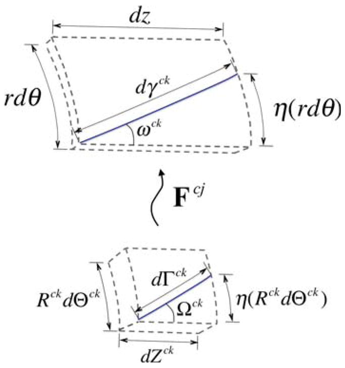
Depiction of the kinematics of an individual fiber from the stress-free configuration to the loaded configuration

$$\begin{array}{l}tan{\mathrm{\Omega }}^{jk}=\frac{\eta (R^{jk}\text{d}{\mathrm{\Theta }}^{jk})}{\text{d}{Z}^{jk}}=\eta \text{and}\\ tan{\omega }^{jk}=\frac{\eta (r\text{d}\theta )}{\text{d}z}=tan{\mathrm{\Omega }}^{jk}\frac{r\text{d}\theta }{\text{d}z}=tan{\mathrm{\Omega }}^{jk}\frac{2\pi r(s)}{\ell (s)}\end{array}$$ (4)

Thus, in general,

$$\stackrel{\sim }{\omega }={tan}^{-1}\left[\frac{2\pi r(s)}{\ell (s)}tan\stackrel{\sim }{\mathrm{\Omega }}\right].$$ (5)

In addition, given axisymmetry and neglecting variation along the vessel length, the stretch of any fiber,

$$\begin{array}{l}{\stackrel{\sim }{\lambda }}_f=\frac{\text{d}\gamma }{\text{d}\stackrel{\sim }{\mathrm{\Gamma }}}\\ =\{\begin{array}{ll}\frac{\text{d}z}{\text{d}\stackrel{\sim }{\mathrm{\Gamma }}cos(\omega (\stackrel{\sim }{\mathrm{\Omega }}))}=\frac{\ell (s)}{\stackrel{\sim }{\mathrm{\Gamma }}cos(\omega (\stackrel{\sim }{\mathrm{\Omega }}))}\hfill & \text{for}0\le \stackrel{\sim }{\mathrm{\Omega }}\le 45°\hfill \\ \frac{r\text{d}\theta }{\text{d}\stackrel{\sim }{\mathrm{\Gamma }}sin(\omega (\stackrel{\sim }{\mathrm{\Omega }}))}=\frac{2\pi r(s)}{\stackrel{\sim }{\mathrm{\Gamma }}sin(\omega (\stackrel{\sim }{\mathrm{\Omega }}))}\hfill & \text{for}45°\le \stackrel{\sim }{\mathrm{\Omega }}\le 90°\hfill \end{array}\end{array}$$ (6)

where Γ̃ is the effective stress-free length of a fiber over the entire radius and length of the vessel, in contrast to dΓ̃, which is the stress-free length over the local neighborhood about a point. Thus, given specific values for r and ℓ that define the current configuration, the fiber stretch λ̃_f and fiber angle ω̃ may be calculated for all possible combinations of Γ̃ and Ω̃ in the {Γ̃, Ω̃}-space via Eqs. (5) and (6).

In traditional vascular mechanics, one typically considers three configurations: a loaded configuration β_t, a traction-free (unloaded) configuration β_u, and a (nearly stress-free) reference configuration β_o (Fig. 3). Here, the stress-free configuration is approximated by an excised arterial ring that ‘springs open’ when cut radially to relieve a large part of the residual stress (Chuong and Fung 1986). As all three configurations are measurable, this approach is experimentally tractable. For inflation and extension of a residually stressed axisymmetric tube, the map X_o(R, Θ, Z)↦ p(ρ, ϑ, ζ) is defined as ρ = ρ(R), ϑ = (π/Θ_o)Θ, and ζ = ΛZ and the map p(ρ, ϑ, ζ) ↦ x(r, θ, z) is defined as r = r(ρ), θ = ϑ, and z = λ_zζ. Thus, the map X_o(R, Θ, Z) ↦ x(r, θ, z) is defined as r = r(R), θ= (π/Θ_o)Θ, and z = λ_zΛZ which has the deformation gradient with components [F] = diag [(∂r/∂R), (πr/Θ_oR), (λ_zΛ)] in cylindrical coordinates. Whereas the radially cut configuration β_o is a convenient and experimentally tractable configuration, it is not necessarily stress-free at all points; i.e., in β_o the local neighborhoods for all points X̂(R̂, Θ̂, Ẑ) are not necessarily in their natural configuration κ_n for the mixture; nor are all points in the natural configurations ${\kappa }_n^j$ for any constituent j. It is important to note, however, that the natural configurations κ_n, ${\kappa }_n^j,{\kappa }_n^{jk}$, and {κ̃_n} are not experimentally tractable. Rather, we must prescribe the distribution of each constituent over the space of all possible natural configurations {κ̃_n} and calculate β_o and β_u using an appropriate stress response function. These predicted values for β_o and β_u may then be compared to experimental data.

Fig. 3.

Traditional kinematics for blood vessel mechanics which considers a loaded configuration β_t, a traction-free (unloaded) configuration β_u, and a (nearly) stress-free configuration β_o that results from imposing a single radial cut in the traction free configuration

2.2 Stress response

The balance of linear momentum for each constituent class and mixture on the whole requires that

$$\begin{array}{l}\text{div}{({\mathbf{T}}^j)}^{\text{T}}+{\rho }^j{\mathbf{b}}^j+{\mathbf{p}}^j+{\stackrel{.}{m}}^j{\mathbf{v}}^j={\rho }^j{\mathbf{a}}^j\text{and}\\ \text{div}{(\mathbf{T})}^{\text{T}}+\rho \mathbf{b}=\rho \mathbf{a},\end{array}$$ (7)

respectively, where ρ^j is the mass density, v^j the velocity, ṁ^j the (net) local mass production per unit volume, T^j the Cauchy stress, b^j the body force, p^j momentum exchanges that arise between constituents, and a^j the acceleration for each constituent class j (which includes all members k) and ρ is the density, T the Cauchy stress, b the body force, and a the acceleration for the mixture as a whole (Humphrey and Rajagopal 2002). For a constrained mixture undergoing a quasi-static process, in the absence of body forces, Eqs. (7)₁ and (7)₂ reduce to div(T^j)^T + p^j +ṁ^jv = 0 and div(T)^T = 0, respectively. Humphrey and Rajagopal (2002) note, however, the difficulty in defining traction boundary conditions in terms of the ‘partial’ stresses T^j and in measuring the momentum exchanges that arise between constituents, and suggest an alternative approach wherein one defines the total mixture stress; in this manner, one need only solve the boundary value problem on the mixture (Eq. (7)₂), without concern with the partial stress boundary condition (Eq. (7)₁). Thus, let the stress of the mixture at any point be described by a simple rule of mixtures (Gleason et al. 2004a; Brankov et al. 1975) as

$$\mathbf{T}=\sum _j\left[\underset{\left\{\stackrel{\sim }{\kappa }\right\}}{\int }{\mathrm{\Phi }}^j(\stackrel{\sim }{\kappa };r)[{\mathbf{T}}^j(\stackrel{\sim }{\mathbf{F}})+{\mathbf{T}}_{\text{act}}^j(\stackrel{\sim }{\mathbf{F}})]\text{d}\stackrel{\sim }{\kappa }\right]$$ (8)

where T^j(F̃) = −p^jI + 2F̃ (∂Ŵ^j/∂C̃) (F̃)^T is the Cauchy stress for each ‘passive’ constituent j with deformation gradient F̃ (modeled as an elastic material), ${\mathbf{T}}_{\mathit{act}}^j(\stackrel{\sim }{\mathbf{F}})$ is the ‘active’ contribution to the Cauchy stress associated with cellular contraction, C̃ is the right Cauchy–Green strain tensor, [C̃] = [F̃(F̃)^T] = diag{(λ̃_r)², (λ̃_θ)², (λ̃_z)²}, Ŵ^j is the strain-energy function for constituent class j, and p^j is a Lagrange multiplier due to (local) incompressibility for each constituent. We will consider a mixture of four key structural constituents: elastin (e), collagen (c), smooth muscle (m) and water (w). We will model water as an inviscid fluid, thus T^w = −p^wI (i.e., 2F̃(∂Ŵ^w/∂C̃)(F̃)^T = 0) and

$$\mathbf{T}=-p\mathbf{I}+\sum _j\underset{\left\{\stackrel{\sim }{\kappa }\right\}}{\int }{\mathrm{\Phi }}^j\left[\stackrel{\sim }{\mathbf{F}}\left(\frac{\partial {\widehat{W}}^j}{\partial \stackrel{\sim }{\mathbf{C}}}\right){(\stackrel{\sim }{\mathbf{F}})}^T+{\mathbf{T}}_{\text{act}}^m(\stackrel{\sim }{\mathbf{F}})\right]\text{d}\stackrel{\sim }{\kappa }$$ (9)

where p = Σ_j∫_{κ̃}(Φ^jp^j)dκ̃ is a Lagrange multiplier due to incompressibility on the mixture as a whole, and we consider muscle to be the only constituent with an active contribution to the stress.

For inflation and extension of a long, straight, axisymmetric tube equilibrium require that T_rθ = T_rz = 0 and ∂T_rr/∂r + (T_rr − T_θθ)/r = 0. Noting that T_rr(r_i) = −P the luminal pressure and T_rr(r_o) = 0, equilibrium requires that

$$P=\underset{r_i}{\overset{r_o}{\int }}({\widehat{T}}_{\theta \theta }-{\widehat{T}}_{rr})\frac{\text{d}r}{r}.$$ (10)

where T̂ = T + pI, the second term in Eq. (9), is the so-called ‘extra’ stress due to the deformation. Axial equilibrium requires that axial force maintaining the in vivo axial extension is $f=2\pi {\int }_{r_i}^{r_o}{T}_{zz}r\text{d}r$, which can be written as

$$f=\pi \underset{r_i}{\overset{r_o}{\int }}(2{\widehat{T}}_{zz}-{\widehat{T}}_{\theta \theta }-{\widehat{T}}_{rr})r\text{d}r+\pi r^{2}P(1-\xi ),$$ (11)

where ξ = 1 or 0 for a closed or open ended tube, respectively; see Humphrey (2002). For ex vivo biomechanical testing, ξ = 1.

As noted above, we seek to prescribe local natural configurations of each constituent and predict the global unloaded configuration β_u and (nearly) stress-free configurations β_o of the mixture. To find β_u, we set P = 0 and f = 0 in Eqs. (10) and (11), and solve for r_i ≡ ρ_i and ℓ = L_u; r_o ≡ ρ_o, and thus, the thickness H_u may be determined from the incompressibility constraint. If we impose a single radial cut in an unloaded vessel, the bending moment, M, is given as

$$\begin{array}{l}M=\underset{r_i}{\overset{r_o}{\int }}(-p+{\widehat{T}}_{\theta \theta })r\text{d}r,\\ \text{where}p(r)={\widehat{T}}_{rr}+P-\underset{r_i}{\overset{r}{\int }}\frac{{\widehat{T}}_{\theta \theta }-{\widehat{T}}_{rr}}{r}\text{d}r.\end{array}$$ (12)

To determine β_o, following Rachev (1997), we set P = 0, f = 0, and M = 0, and solve for r_i ≡ R_i, ℓ ≡ L_o, and Θ_o; again, R_o, and thus the thickness H_o, may be determined from incompressibility.

2.3 Constitutive equations

We will model elastin as a neo–Hookean material; thus,

$${\widehat{W}}^e=2b^e(I_{\stackrel{\sim }{C}}-3),$$ (13)

where b^e is the elastic modulus and I_C̃ = tr(C̃) = C̃_rr + C̃_θθ+ C̃_zz is the first invariant of C̃.

We model muscle as a transversely isotropic material with a circumferentially preferred direction; thus

$${\widehat{W}}_{\mathit{pas}}^m=b^m(I_{\stackrel{\sim }{\mathbf{C}}}-3)+\frac{b_1^m}{4b_2^m}\left\{exp\left(b_2^m{\left({\stackrel{\sim }{C}}_{\theta \theta }-1\right)}^2\right)-1\right\}$$ (14)

where b^m, $b_1^m$, and $b_2^m$ are material parameters.

We consider collagen to be comprised of a distribution of fibers with fiber orientations ω̃ ∈ [0, 90] and fiber stretches λ̃_f. For each fiber, we let

$${\widehat{W}}^c=\frac{b_1^c}{2b_2^c}\left[exp\left(b_2^c{\left({\stackrel{\sim }{\lambda }}_f^2-1\right)}^2\right)-1\right].$$ (15)

where $b_1^c$ and $b_2^c$ are material parameters. Each fiber is oriented in the Z̃–Θ̃ plane, λ̃_f = γ/Γ̃ is the stretch of the fiber, where ${\stackrel{\sim }{\lambda }}_f^2={\mathbf{M}}^n·\stackrel{\sim }{\mathbf{C}}{M}^n,{\mathbf{M}}^n=sin({\mathrm{\Omega }}_n^j){\mathbf{e}}_{\theta }+cos({\mathrm{\Omega }}_n^j){\mathbf{e}}_z$; thus, ${\stackrel{\sim }{\lambda }}_f^2={\stackrel{\sim }{C}}_{\theta \theta }{sin}^2(\stackrel{\sim }{\mathrm{\Omega }})+2{\stackrel{\sim }{C}}_{\theta z}sin({\mathrm{\Omega }}_n^j)cos({\mathrm{\Omega }}_n^c)+{\stackrel{\sim }{C}}_{zz}{cos}^2(\stackrel{\sim }{\mathrm{\Omega }})$, where Ω̃ denotes the angle between the fiber direction and Z̃ axis in the reference configuration κ̃_n, γ is the length of the fiber in the loaded configuration, Γ̃ is the unloaded length of fibers oriented in the direction Ω̃; note that Γ̃ is similar to the ‘fiber engagement’ length described by Lanir (1983) and others. Note, that, we assume that the collagen fibers are embedded in the amorphous matrix described by the isotropic terms in Eqs. (13) and (14). Note too that we only consider distribution functions that possess symmetry about the r – z plane and the r – θ plane; thus the limits of integration in Eq. (15) represent the first quadrant, which is repeated in the 2nd, 3rd, and 4th quadrant.

The active smooth muscle behavior will be modeled following Rachev and Hayashi (1999) as

$${\mathbf{T}}_{\text{act}}^m=T_{\text{act}}{\stackrel{\sim }{\lambda }}_{\theta }\left[1-{\left(\frac{{\lambda }_M-{\stackrel{\sim }{\lambda }}_{\theta }}{{\lambda }_M-{\lambda }_o}\right)}^2\right]{\mathbf{e}}_{\theta }\otimes {\mathbf{e}}_{\theta }$$ (16)

where λ_M is the stretch at which the contraction is maximum, λ₀ is the stretch at which active force generation ceases, T_act is a parameter associated with the degree of muscle activation, and e_θ is the base vector in the circumferential direction in the loaded configuration.

2.4 Evolution equations

For the simulations herein, we assume that the material parameters for each constituent class remain constant for all material produced or removed. Thus, to quantify growth and remodeling, what remains is to quantify how the distribution of mass over all possible reference configurations Φ^j (R̃, L̃; r, s) changes with position and time as the tissue grows and remodels. Toward this end, we must quantify the rate of production and removal of each constituent and the mechanical state (i.e., natural configuration) of all material being produced.

2.4.1 Growth and turnover kinetics

Mass balance for each constituent class j within a mixture and for the mixture as a whole requires that

$$\begin{array}{l}\frac{\partial {\rho }^j}{\partial s}+\text{div}({\rho }^j{\mathbf{v}}^j)={\stackrel{.}{m}}^j\text{and}\\ \frac{\partial \rho }{\partial s}+\text{div}(\rho \mathbf{v})=0,\end{array}$$ (17)

respectively (Humphrey and Rajagopal 2002). Assuming that the mixture density does not vary significantly with position and time, (17)₂ reduces to div(v) = 0. For a constrained mixture each constituent, including water, is ‘constrained’ to deform together; thus, each constituent has the same velocity as the mixture (i.e., v^j = v and diυ(v^j) = diυ(v)) and for a homogeneous material Eq. (17)₁ reduces to ∂ρ^j/∂s = ṁ^j.

Consider the local neighborhood κ_t about point x(r, θ z) at time s = 0 ≡ s₀ in the loaded axisymmetric, cylindrical configuration that has mass dm(s₀, r) ≡ dm₀, volume dυ(s₀, r) = dυ₀, and mass fractions ${\phi }_o^j(s_o,r)=\text{d}{m}_o^j/\text{d}{m}_o$ within the region at s₀, where $\text{d}{m}_o^j=\text{d}{m}^j(s_o,r)$ is the mass of constituent j at s = 0. The mass density of the mixture and the constituents over this region are ρ₀(r) = dm₀/dυ₀ and ${\rho }_o^j(r)={\phi }_o^j\text{d}{m}_o/\text{d}{\upsilon }_o=\text{d}{m}_o^j/\text{d}{\upsilon }_o$. At a later time s, following some constituent turnover, including addition or loss of mass (i.e., growth or atrophy), the region may have a new mass, dm(r, s) ≡ α (r, s)dm₀(r), new volume dυ(r, s) in the current configuration, and new mass fractions ${\phi }^j(r,s)\equiv [{\alpha }^j(r,s)/\alpha (r,s)]{\phi }_o^j(r)$ where ${\alpha }^j(r,s)=\text{d}{m}^j(r,s)/\text{d}{m}_o^j(r)$. If the mixture density remains nearly constant, (i.e., ρ (r) ≅ ρ₀(r) = constant ∀ r, s, c.f., Rodriguez et al. 1994), then dm/dm₀ = dυ/dυ₀ ≡ α (r, s) and ${\rho }^j(r,s)=\frac{{\alpha }^j(r,s)}{\alpha (r,s)}{\rho }_o^j(r)$. Note too, that since we assume material incompressibility, the volume of this neighborhood in the natural configuration (of the mixture) κ_n, denoted dV (s, r), is equal to the volume in the loaded configuration dυ(r, s); thus dV (s₀, r) ≡ dV₀ = dυ₀ and dV (s, r) ≡ dV = dυ. Since we are adding mass (and volume), dV ≠ dV₀, we let

$$\frac{\text{d}V}{\text{d}{V}_o}\left(=\frac{\text{d}\upsilon }{\text{d}{\upsilon }_o}=\frac{\text{d}m}{\text{d}{m}_o}=\alpha (s,r)\right)=det{\mathbf{F}}_g={\lambda }_{rg}{\lambda }_{\theta g}{\lambda }_{zg}$$ (18)

where [F_g] = diag{λ_rg, λ_θg, λ_zg} is a deformation gradient for the mapping of points from their original natural configuration κ_n (s = 0) to their current natural configuration κ_n (s), where we consider only axisymmetric growth (Fig. 4). λ_ig (i = r, θ, z)are the so-called growth stretch ratios; see Rodriguez et al. (1994), Rachev (1997), and Taber and Eggers (1996) which may be written

Fig. 4.

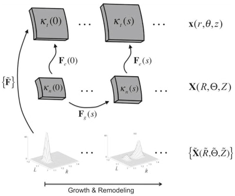
Kinematics for the volumetric and constrained mixture approaches. Volumetric growth is described by tracking changes in the local stress-free configuration, which is quantified by prescribing evolution equations for the ‘growth’ deformation F_g. The elastic deformation F_e is the gradient of the mapping of points from the current stress-free configuration to the current loaded configuration. In the constrained mixture approach, one tracks the evolution of the distribution of mass over all possible combinations of constituent stress-free states

$${\lambda }_{gr}=\frac{\text{d}R(s)}{\text{d}R(0)},{\lambda }_{g\theta }=\frac{R(s)}{R(0)},\text{and}{\lambda }_{gz}=\frac{\text{d}Z(s)}{\text{d}Z(0)}.$$ (19)

In the traditional volumetric approach, one proceeds by prescribing evolution equations for ∂λ_ig/∂t. Here, however, we take a different approach; we prescribe the overall rate of change in mass (or volume) with respect to time and prescribe the mechanical state in which new constituents are laid down. Thus, rather than prescribing the evolution of λ_ig, we predict these values.

The rate of change of mass of this region may be written as

$$\begin{array}{l}\frac{\partial (\text{d}m)}{\partial s}=\sum _j\frac{\partial (\text{d}{m}^j)}{\partial s}\\ =\sum _j\left[{\left(\frac{\partial (\text{d}{m}^j)}{\partial s}\right)}_{\text{prod}}-{\left(\frac{\partial (\text{d}{m}^j)}{\partial s}\right)}_{\mathit{rem}}\right]\end{array}$$ (20)

or equivalently,

$$\begin{array}{l}\frac{\partial \alpha (r,s)}{\partial s}=\sum _j{\phi }_o^j\frac{\partial {\alpha }^j(r,s)}{\partial s}\\ =\sum _j{\phi }_o^j\left[{\left(\frac{\partial {\alpha }^j(r,s)}{\partial s}\right)}_{\text{prod}}-{\left(\frac{\partial {\alpha }^j(r,s)}{\partial s}\right)}_{\text{rem}}\right].\end{array}$$ (21)

In general,

$${\left(\frac{\partial {\alpha }^j}{\partial s}\right)}_{\text{rem}}={\widehat{q}}^j\left({\alpha }^j(r,s),(\stackrel{\sim }{\sigma }(r,s)-{\stackrel{\sim }{\sigma }}^h),\cdots ;r\right)$$ (22)

where q̂^j (α^j, σ̃ − σ̃^h, ···) allows for the rate to depend on the mass of material present α^j(s), a stress difference(s), (σ̃(s) − σ̃^h), where σ̃(s) is some stress measured relative to its homeostatic value, σ̃^h, among other factors. Because ∂α^j/∂s, (∂α^j/∂s)_prod, (∂α^j/∂s)_rem are related through (20), we must prescribe two of these three rates to specify fully the kinetics of turnover. Let us prescribe the net growth rate of j, in general, as

$$\frac{\partial {\alpha }^j}{\partial s}={\widehat{g}}^j\left({\alpha }^j(r,s),(\stackrel{\sim }{\sigma }(r,s)-{\stackrel{\sim }{\sigma }}^h),\cdots ;r\right).$$ (23)

Thus, the rate of production of j is

$${\left(\frac{\partial {\alpha }^j}{\partial s}\right)}_{\text{prod}}={\widehat{q}}^j(r,s)+{\widehat{g}}^j(r,s).$$ (24)

For our illustrative examples, we let

$$\begin{array}{l}{\widehat{q}}^j(r,s)={\alpha }^j(r,s)\left(k_B^j+q^j(\mathbf{T},{\tau }_w)\right)\text{and}\\ {\widehat{g}}^j(r,s)={\alpha }^j(r,s)g^j(\mathbf{T},{\tau }_w)\end{array}$$ (25)

where k_B is a constant that yields a ‘basal’ rate of constituent turnover, and we let

$$\begin{array}{l}{q}^j(r,s)=a_{q1}^j\sqrt{{\left(\frac{T_{\text{act}}(s)}{T_B}-1\right)}^2}\\ \times \left[a_{q2}^j\sqrt{{\left(\frac{T_{\theta \theta }(r,s)}{T_{\theta \theta }^T}-1\right)}^2}+1\right]\end{array}$$ (26)

and

$$\begin{array}{l}{\widehat{g}}^j(r,s)=a_{g1}^j\left[\left(\frac{T_{\mathit{act}}(s)}{T_B}-1\right)+a_{g2}^j\left(\frac{\langle T_{\theta \theta }\rangle }{\langle T_{\theta \theta }^T\rangle }-1\right)\right]\\ \times \left[a_{g3}^j\left(\frac{T_{\theta \theta }(r,s)}{T_{\theta \theta }^T}-1\right)+1\right];\end{array}$$ (27)

here $a_{q1}^j,a_{q2}^j,a_{g1}^j,a_{g2}^j$ and $a_{g3}^j$ are kinetic parameters. Thus, we hypothesize that the rates of turnover and growth are mediated by mean and local circumferential stress and degree of smooth muscle activation. Constituent removal (i.e., turnover) is mediated by the absolute value of the difference of muscle activation and circumferential stress from basal values and reaches a basal rate when T_act is restored. Thus, increases or decreases in these values result in increased turnover. Growth (i.e., net change in mass) is mediated by the muscle activation parameter T_act, the mean circumferential stress 〈T_θθ〉 = P(s)a(s)/h(s), and local circumferential stress T_θθ. The terms in the first set of square brackets in Eq. (27) are not functions of position while the first term in the second set of brackets is a function of position. Steady state is achieved when the terms in the first set of square brackets reach zero; the term in the second set of square brackets serves to control local differences in stress-mediated growth across the wall.

The rate of change of mass density of each constituent, ṁ^j, is related to α^j and α via the relation

$${\stackrel{.}{m}}^j=\frac{\text{d}}{\text{d}s}\left(\frac{\text{d}{m}^j}{\text{d}\upsilon }\right)=\frac{\text{d}}{\text{d}s}\left(\frac{{\alpha }^j}{\alpha }\frac{\text{d}{m}_o^j}{\text{d}{\upsilon }_o}\right)={\rho }_o\frac{\text{d}}{\text{d}s}\left(\frac{{\alpha }^j}{\alpha }\right).$$ (28)

Thus, ṁ^j is proportional to the rate of change of α^j/α.

2.4.2 Mechanical state of produced and removed material

In biological tissue, material is produced and removed in the loaded configuration, under stress and strain; thus, in our simulations, material is laid down in the in vivo, loaded configuration under stress and strain. In particular, we assume that the new material gets laid down in a homeostatic state of strain.

For growth and turnover of elastin and smooth muscle, we adopt the approach of Gleason and Humphrey (2005b). Briefly, as new material is produced, we require constituent j to be deposited via the homeostatic distribution ${\mathrm{\Lambda }}_h^j({\stackrel{\sim }{\lambda }}_{\theta },{\stackrel{\sim }{\lambda }}_z)$. Rather than prescribing the functional form of ${\mathrm{\Lambda }}_h^j({\stackrel{\sim }{\lambda }}_{\theta },{\stackrel{\sim }{\lambda }}_z)$, we prescribe the functional form of the distribution of natural configurations $R_h^j(\stackrel{\sim }{R},\stackrel{\sim }{L};r,s)$ that results from laying down new material with the distribution of stretches ${\mathrm{\Lambda }}_h^j({\stackrel{\sim }{\lambda }}_{\theta },{\stackrel{\sim }{\lambda }}_z)$ in the (known) loaded configuration. Although ${\mathrm{\Lambda }}_h^j({\stackrel{\sim }{\lambda }}_{\theta },{\stackrel{\sim }{\lambda }}_z)$ is independent of time, $R_h^j(\stackrel{\sim }{R},\stackrel{\sim }{L};r,s)$ depends on s because the state (2πr(s_p), ℓ(s_p)) wherein it is produced depends on s. We let $R_h^j(\stackrel{\sim }{R},\stackrel{\sim }{L};r,s)$ be described by a beta probability distribution function, with independent variables R̃ and L̃, as

$$\begin{array}{l}{R}_h^j(\stackrel{\sim }{R},\stackrel{\sim }{L};r,s)\\ =\left(\frac{{(\stackrel{\sim }{R}-R_{min}^j(r,s))}^{p_A^j-1}{(R_{max}^j(r,s)-\stackrel{\sim }{R})}^{q_A^j-1}}{B(p_A^j,q_A^j){(R_{max}^j(r,s)-R_{min}^j(r,s))}^{p_A^j+q_A^j-1}}\right)\\ \times \left(\frac{{(\stackrel{\sim }{L}-L_{min}^j(s))}^{p_L^j-1}{(L_{max}^j(s)-\stackrel{\sim }{L})}^{q_L^j-1}}{B(p_L^j,q_L^j){(L_{max}^j(s)-L_{min}^j(s))}^{p_L^j+q_L^j-1}}\right)\end{array}$$ (29)

where $p_A^j,q_A^j,p_L^j$, and $q_L^j$ are shape parameters, B(·, ·)is the beta function, $R_{min}^j(r,s)={\overline{R}}^j(r,s)-\mathrm{\Delta }{R}^j/2,R_{max}^j(r,s)={\overline{R}}^j(r,s)+\mathrm{\Delta }{R}^j/2,L_{min}^j(s)={\overline{L}}^j(s)-\mathrm{\Delta }{L}^j/2$, and $L_{max}^j(s)={\overline{L}}^j(s)+\mathrm{\Delta }{L}^j/2$. R̄^j and L̄^j are mean values of the natural configurations, and ΔR ^j and ΔL^j are the widths of the distribution. If we know the current state (r(s_p), ℓ(s_p)), we can prescribe the mean natural configurations of the distribution as

$${\overline{R}}^j(s_p)=\frac{r(s_p)}{{{\lambda }_{\theta }^j|}_h}\text{and}{\overline{L}}^j(s_p)=\frac{\ell (s_p)}{{{\lambda }_z^j|}_h},$$ (30)

where ${{\lambda }_{\theta }^j|}_h$ and ${{\lambda }_z^j|}_h$ are the mean value of the preferred homeostatic stretch distribution.

For collagen, we let the fibers be laid down at a homeostatic distribution of fiber angles described via a sum of normal distribution functions, given as

$$\begin{array}{l}\text{A}(\stackrel{\sim }{\omega })=\left[\frac{1}{2{\sum }_p{a}_p}\right]\sum _p\frac{a_p}{{\sigma }_p\sqrt{2\pi }}\\ \times \sum _{n=1}^2\{exp\left[\frac{-(\stackrel{\sim }{\omega }+{(-1)}^n{\mu }_p)}{2{\sigma }_p^2}\right]\\ +exp\left[\frac{-(\stackrel{\sim }{\omega }+{(-1)}^n({\mu }_p-180))}{2{\sigma }_p^2}\right]\}\end{array}$$ (31)

where ω̃ ∈ [0, 90°] is the angle between a fiber and the z axis in the loaded configuration, and μ_p and σ_p are the mean and standard deviation of normal distribution p. In addition, we will assume that at each fiber angle, ω̃, the fibers are laid down at a homeostatic distribution of stretches, ${\mathrm{\Lambda }}_h^c({\stackrel{\sim }{\lambda }}_f,\stackrel{\sim }{\omega };s)$. As in the case for elastin and smooth muscle, rather than prescribing the distribution of in vivo stretches and mapping these stretches back to a reference state, we will simply prescribe the distribution of fiber lengths (dΓ̃) in the reference state; let this distribution be denoted as B(dΓ̃, Ω̃; r, s), via a beta distribution function, as

$$\begin{array}{l}\text{B}(\text{d}\stackrel{\sim }{\mathrm{\Gamma }},\stackrel{\sim }{\mathrm{\Omega }};r,s)\\ =\left(\frac{{\text{(d}\stackrel{\sim }{\mathrm{\Gamma }}-\text{d}{\mathrm{\Gamma }}_{min}(\stackrel{\sim }{\omega }))}^{p^c(\stackrel{\sim }{\omega })-1}{(\text{d}{\mathrm{\Gamma }}_{max}(\stackrel{\sim }{\omega })-\text{d}\stackrel{\sim }{\mathrm{\Gamma }})}^{q^c(\stackrel{\sim }{\omega })-1}}{B(p^c(\stackrel{\sim }{\omega }),q^c(\stackrel{\sim }{\omega })){(\text{d}{\mathrm{\Gamma }}_{max}(\stackrel{\sim }{\omega })-\text{d}{\mathrm{\Gamma }}_{min}(\stackrel{\sim }{\omega }))}^{p^c(\stackrel{\sim }{\omega })+q^c(\stackrel{\sim }{\omega })-1}}\right)\end{array}$$ (32)

where we recall that ω̃ = ω̃(Ω̃; s), p^c(ω̃), and q^c(ω̃) are shape parameters, dΓ_max(ω̃, s) and dΓ_min(ω̃, s) are the maximum and minimum values of dΓ̃ (i.e., B(dΓ̃, Ω̃; r, s) = 0 for dΓ̃ > dΓ_max and dΓ̃ < dΓ_min), and B(·, ·) is the beta function. Note dΓ_max = dΓ_mean + ΔdΓ/2 and dΓ_min = dΓ_mean − ΔdΓ/2, where dΓ_mean is the mean value and ΔdΓ the width of the dΓ̃ distribution function.

The distribution of mass over all combinations of fiber angle and fiber stretch may be given as

$${\widehat{\text{R}}}^j(\stackrel{\sim }{\mathrm{\Gamma }},\stackrel{\sim }{\mathrm{\Omega }};r,s)={\text{A}}^j(\stackrel{\sim }{\omega }(\stackrel{\sim }{\mathrm{\Omega }});r,s){\text{B}}^j(\stackrel{\sim }{\mathrm{\Gamma }},\stackrel{\sim }{\mathrm{\Omega }};r,s)$$ (33)

This distribution function has the properties

$$\begin{array}{l}{\widehat{\text{R}}}^j(\stackrel{\sim }{\mathrm{\Gamma }},\stackrel{\sim }{\mathrm{\Omega }})>0\forall \omega ,{\lambda }_f\text{and}\\ \int \underset{\stackrel{\sim }{\mathrm{\Gamma }},\stackrel{\sim }{\mathrm{\Omega }}}{\int }{\widehat{\text{R}}}^j(\stackrel{\sim }{\mathrm{\Gamma }},\stackrel{\sim }{\mathrm{\Omega }})\frac{\partial \stackrel{\sim }{\omega }}{\partial \stackrel{\sim }{\mathrm{\Omega }}}\text{d}\stackrel{\sim }{\mathrm{\Omega }}\text{d}\stackrel{\sim }{\mathrm{\Gamma }}=1.\end{array}$$ (34)

Notice that the ‘homeostatic’ distribution function R̂^c(Γ̃ Ω̃; r, s) captures (qualitatively) the fiber orientations observed in these vessels, as well as the observation that different fibers become loaded (i.e., recruited) in different loaded configurations (Fig. 5).

Fig. 5.

a Distribution of in vivo collagen fiber angles and stretches, b confocal microscopy image of collagen fibers from a mouse carotid artery under in vivo loading conditions

3 Illustrative results

The governing equations are the kinematic equations (3), the constitutive equations (9), and (13)–(16), equilibrium equations (10) and (11), the kinetic equations (22)–(27) which describe the rate of constituent turnover and growth, and Eqs. (29)–(33) which describe the mechanical state of newly produced material. Based on data from mouse carotid arteries (Gleason et al. 2007), we prescribe the initial mean values (over the cardiac cycle): the in vivo inner radius a_o = 250 μm, in vivo thickness h_o = 24.16 μm, and in vivo axial length ℓ_o = 2πa_o = 1.57 mm. Structural and material parameters were determined by fitting this constitutive model to experimental data from mouse common carotid arteries from Gleason et al. (2007), following the methods described in Hansen et al. (2009). The structural parameters for the mechanical state in which constituents are laid down are ${{\lambda }_{\theta }^e|}_h=1.98,{{\lambda }_z^e|}_h=2.25,{{\lambda }_{\theta }^m|}_h=1.72,{{\lambda }_z^m|}_h=1.88,{{\lambda }_f^c|}_h=1.34$ , ω̄₁ = 0°, and ω̄₁ = 28°, and the material parameters are b^e = 103.95 kPa, b^m = 0.362 kPa, $b_1^m=10.15\text{kPa},b_{\text{2}}^m=0.402,b_1^c=751.34\text{kPa},b_2^c=1.332$, T_B = 363 kPa, λ_M = 2.1, and λ₀ = 0.8. Pressure-diameter, axial force-pressure, and mid-wall stress-strain plots show that these material parameters capture the salient feature of large arteries (Fig. 6). Kinetic parameters used for each simulation are listed below. We solved this system of equations numerically by discretizing the radius and using an implicit time-step implemented in MatLab 7.4. We also discretized the space of all possible natural configurations κ̃_n (i.e., the R̃ − L̃ -space for elastin and muscle and the Γ̃ − Ω̃-space for collagen).

Fig. 6.

a Simulated results from a typical pressure-diameter test of a typical mouse carotid artery, b simulated axial force-pressure test, and c mean circumferential stress strain data for mixture and for constituents using proposed constitutive models with prescribed structural and material parameters

Given the initial loaded configuration r(0) and ℓ_o, we calculated values for the initial distribution functions Φ^j (κ̃_n, r, s = 0) (by setting r(s_p) = r(0) and ℓ(s_p) = ℓ_o in Eqs. (29), (30), and (33)), the deformation gradient, and the components of stress for each constituent at each node in each discretized 2-D space (i.e., R̃ − L̃ -space and Γ̃ − Ω̃-space) at each radial location. The components of the ‘extra’ stress were calculated by integrating the second term on the right hand side of Eq. (9); for elastin and muscle, equation (9) represents a surface integral over R̃ and L̃; for collagen, equation (9) becomes a double integral over Γ̃ and Ω̃. The Lagrange multiplier was calculated via Eq. (12)₂, and the total Cauchy stress was calculated via Eq. (9).

At time s = 0⁺, we imposed the change in applied loads to P(s) = βP_o, Q(s) = εQ_o, and ℓ(s) = δℓ_o. To impose the assumption that the vessel aims to restore wall shear stress via vasoregulation, we first determined the vasoactive range of radii at any time s, by solving Eq. (10) for the inner radius with $T_{\text{act}}=T_{\text{act}}^{max}$ and T_act = 0; this yields the maximally constricted and maximally dilated inner radii ( $r_i^{min}$ and $r_i^{max}$), respectively. The (‘target’) inner radius that restores wall shear stress is $r_i^{\text{targ}}={\epsilon }^{1/3}{r}_i(0^{-})$, as shown in Gleason et al. (2004a). If $r_i^{\text{targ}}>r_i^{max}$, then the maximal dilation is not sufficient to restore wall shear stress, and we set T_act(s) = 0 and $r_i(s)=r_i^{max}$. If $r_i^{\text{targ}}<r_i^{min}$ then the maximal constriction is not sufficient to restore wall shear stress, and we set $T_{\text{act}}(s)=T_{\text{act}}^{max}$ and $r_i(s)=r_i^{min}$. If $r_i^{\text{targ}}\in [r_i^{min},r_i^{max}]$, then $T_{\text{act}}(s)\in [0,T_{\text{act}}^{max}]$; in this case, we set $r_i(s)=r_i^{\text{targ}}$ and solve Eq. (10) for T_act(s). Given this new configuration and activation, we calculated T(s) via Eqs. (9) and (12)₂.

Given the calculated values for T_θθ(s) and T_act(s), the amount of (normalized) mass produced ( $\text{d}{\alpha }_{\text{prod}}^j(s)$) and removed ( $\text{d}{\alpha }_{\text{rem}}^j(s)$) for the next time step (ds) was calculated via Eqs. (22)–(27). The new distribution of mass at each radial location is given as,

$$\begin{array}{l}{R}^j({\stackrel{\sim }{\kappa }}_n;r,s+\text{d}s)\\ =\frac{({\alpha }^j(s)+\text{d}{\alpha }_{\text{rem}}^j(s))R^j({\stackrel{\sim }{\kappa }}_n;r,s)+\text{d}{\alpha }_{\text{prod}}^j(s)R_h^j({\stackrel{\sim }{\kappa }}_n;r,s)}{{\alpha }^j(s+\mathrm{\Delta }s)}\end{array}$$ (35)

where $R_h^j({\stackrel{\sim }{\kappa }}_n;r,s)$ is calculated via Eq. (29) for elastin and muscle, Eq. (33) for collagen, and where the configuration in which the material is produced (r(s_p)and ℓ(s_p)) is the current configuration (r(s) and ℓ(s)). Finally, Φ^j(κ̃_n; r, s + ds) = φ^j(r, s + ds) R^j(κ̃_n; r, s + ds). Next, we let s = s + ds, proceeded to the next time step, and repeated these steps for a specified number of time-steps.

3.1 Altered flow

For all altered flow simulations, we let ε = 2.0 and β = δ = 1.0; that is, a two-fold increase in flow with no change in pressure or axial length. We considered two illustrative cases: one in which all constituents turnover at equal rates (EQUAL RATES) and one in which constituents are turned over at representative physiological rates (PHYSIOLOGICAL RATES).

3.1.1 Equal rates

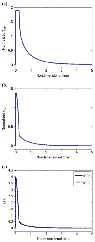
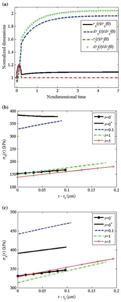
We let $k_b^e=k_b^m=k_b^c=0.1,a_{q1}^e=a_{q1}^m=a_{q1}^c=1.0,a_{q2}^e=a_{q2}^m=a_{q2}^c=1.0,a_{g1}^e=a_{g1}^m=a_{g1}^c=0.1,a_{g2}^e=a_{g2}^m=a_{g2}^c=10.0$, and $a_{g3}^e=a_{g3}^m=a_{g3}^c=1.0$. Following altered flow, smooth muscle cell relaxation (via reduction in T_act) caused the vessel to dilate; c.f., r_i(s)/r_i (0⁻) at s = 0⁻ before vasodilation and s = 0⁺ after dilation (Fig. 7a). The vessel wall thinned with dilation (via incompressibility), and the total circumferential and axial stress across the vessel wall increased (Fig. 7b, c). The growth is governed by (T_act/T_B − 1), (〈T_θθ(s)〉/〈T_θθ〉^T − 1), and ( $T_{\theta \theta }(r,s)/T_{\theta \theta }^T-1$) via Eqs. (26) and (27). Following dilation, smooth muscle cells were fully relaxed (i.e., T_act=0 and (T_act/T_B − 1) = −1), and the shear stress was not completely restored to the homeostatic value (Fig. 8a). Also at s = 0⁺, (〈T_θθ(s)〉/〈T_θθ〉^T − 1) = 0.15 (Fig. 8b). Since $a_{g2}^j=10.0$, the term in the first set of square brackets in Eq. (27) equaled 0.5 at s = 0⁺. The local stress increased to different extents at different locations across the vessel wall; thus, the term in the second set of square brackets in Eq. (27) varied across the wall, decreasing monotonically from the inner to outer wall (see Fig. 7b). Thus, the net effect of (T_act/T_B − 1), (〈T_θθ(s)〉/〈T_θθ〉^T − 1), and ( $T_{\theta \theta }(r,s)/T_{\theta \theta }^T-1$) is that g^j was positive immediately following dilation, and the vessel began to accumulate mass to different extents at different radial locations (Fig. 8c). Note that mass accumulation can be delayed by decreasing a_g2; this could cause some initial atrophy before growth occurs. The rate of turnover is governed by (T_act/T_B − 1) and (〈T_θθ(s)〉/〈T_θθ〉^T − 1), according to Eq. (26); following vasodilation, the rate of turnover increased ~2.7-fold, but varied across the wall. As the vessel wall grew and existing constituents were replaced with new constituents with new natural configurations, the vessel wall radius continued to increase. This increased radius and decreased thickness caused the mean and local wall stresses to be increased further. At s = 3.1, the vessel reached the ‘target’ radius of a(s) = 1.26a_o, and the smooth muscle began to contract. As growth and remodeling proceed, T_act asymptotically approached its basal value T_B. The total thickness increased to h/h_o = ε^1/3 = 1.26. Locally, however, since rates of growth varied with radius, there were different levels of local thickening at different locations (see Fig. 7a); thickening was slightly higher at inner versus outer wall locations. The mean and local values of the circumferential and axial stresses were restored to initial values. Mean axial stress and mean circumferential stress both reached a maximum value upon increase in flow at s = 0⁺, and then asymptotically decreased to initial values.

Fig. 7.

Flow: equal rates. a Normalized radius and local thickness at the inner and outer wall versus time. b Circumferential stress distribution and c axial stress distribution at different time-points during growth and remodeling

Fig. 8.

Flow: equal rates. a Normalized muscle activation (T_act/T_B − 1), b mean circumferential stress, and c growth rate versus time

Prior to dilation, the stretches in each constituent were at their homeostatic values. For example, at s = 0⁻, the stretches in the muscle were distributed over the ranges ${\lambda }_{\theta }^m\in [1.71,1.73]$ and ${\lambda }_z^m\in [1.87,1.89]$ (Fig. 9a). Following dilation, as the radius increased the circumferential stretch in muscle increased to ${\lambda }_{\theta }^m\in [1.83,1.85]$ (Fig. 9b); since there is no change in axial length with dilation, the axial stretches remain unchanged. As constituent turnover ensued, newly formed constituents were laid down at the homeostatic values of these stretches. For muscle, newly formed material were laid down at ${\lambda }_{\theta }^m\in [1.71,1.73]$ and ${\lambda }_z^m\in [1.87,1.89]$; thus, at time-points when both existing and newly form constituents coexist, the total mass of muscle became distributed over all possible combinations of in-plane stretches in a bimodal fashion (see Fig. 9c, d). Note too, that material formed immediately after dilation, when a(s) = 1.07a₀, and laid down at the homeostatic stretches becomes stretched further as the vessel continued to increase its radius to a(s) = 1.26a₀. Eventually, as the vessel reached the configuration that restores wall shear stress and is held constant while constituent turnover continued, material at stretches outside of the homeostatic stretches were eventually replaced with material laid down at the homeostatic stretches (Fig. 9e, f).

Fig. 9.

Flow: Equal Rates. Surface describing how muscle is distributed over all possible sets of circumferential and axial stretches at a s = 0⁻, b s = 0⁺, c s = 0.86, d s = 1.73, e s = 4.92, f s = ∞

Similarly, the distribution of collagen over all possible combinations of fiber angle ω̃ and fiber stretch λ̃_f in the in vivo configuration evolved with growth and remodeling. Initially, the mean fiber angles were ω̄₁ = 0° and ω̄₂ = 28°, and the mean stretch of these fibers equaled the homeostatic value ${\lambda }_f^{c1}={\lambda }_f^{c2}=1.34$ (not shown). Upon vasodilation, the fiber angle and fiber stretch ratio deformed to ω̄₂ = 29.7° and ${\lambda }_f^{c2}=1.36$; there was no change in ω̄₁ and since there was no change in vessel length, there was no change in ${\lambda }_f^{c1}$. As new collagen was produced, however, it was laid down at the homeostatic fiber angle and fiber stretch; thus, a bimodal distribution of (between ω̄₂ = 28° and ω̄₂ = 29.7°, in addition to the peak at ω̄₁ = 0°) resulted. Eventually, as the vessel reached the configuration that restored wall shear stress and was held constant and constituent turnover continued, material at fiber orientations and fiber stretches outside of the homeostatic stretches were eventually replaced with material laid down at the homeostatic fiber orientations and fiber stretches.

3.1.2 Physiological rates

In vivo, the rates of growth and turnover of elastin, collagen, and muscle vary significantly. We know, for example, that the rate of turnover of smooth muscle is significantly higher than that of collagen, but that the ratio of total mass of collagen to that of muscle remains nearly constant. This may be simulated in our model by setting $a_{q1}^m=10a_{q1}^c$, still requiring that $a_{g1}^m=a_{g1}^c$. We also know that in adult vertebrates, the rate of production and turnover of elastin is very small compared to that of muscle and collagen. This may be simulated in our model by setting $k_B^e=a_{q1}^e=a_{g1}^e\sim 0$. Thus, we let $k_B^e=a_{q1}^e=a_{g1}^e=0,k_B^m=k_B^c=0.1,a_{q1}^m=10,a_{q1}^c=1.0,a_{q2}^m=a_{q2}^c=1.0,a_{g1}^m=a_{g1}^c=0.1,a_{g2}^m=a_{g2}^c=10.0$, and $a_{g3}^m=a_{g3}^c=1.0$. For physiological rates of growth and turnover, the circumferential and axial stresses approach, but did not completely restore initial values (Fig. 10). In addition, the thickness initially decreased, then thickened to h/h₀ = 1.24, which is less than the ‘target’ value of ε^1/3 = 1.26. Thus, neither 〈T_θθ (s)〉 nor T_act(s) were restored and remained 2% above and 19% below homeostatic values, respectively. The mass fractions of collagen, muscle, and elastin varied with both time and radial location, with the greatest increase in collagen and muscle mass fraction at inner versus outer wall locations (not shown). Therefore, in addition to non-uniform thickening, in this case, the vessel evolved from a homogeneous material to a heterogeneous material.

Fig. 10.

Flow: physiological rates. a Normalized radius and local thickness at the inner and outer wall versus time. b Circumferential stress distribution and c axial stress distribution at different time-points during growth and remodeling

3.2 Altered pressure

For this altered pressure simulation, we let β = 2.0 and ε = δ = 1.0; that is, a twofold increase in pressure with no change in flow or axial length. We performed these simulations at the physiological turnover rates. Following the increase in pressure, the vessel passively distended to enlarge the lumen and simultaneously (within minutes), the smooth muscle activation increased to $T_{\text{act}}=T_{\text{act}}^{max}$ (with act (T_act/T_B − 1) = 1.9, Fig. 11a) due to the lower shear stress that occurs due to the increase in radius and unchanging flow rate. For this large increase in pressure, the maximum smooth muscle activation was not sufficient to restore the inner radius to the ‘target’ value that restores the wall shear stress (Fig. 12a). The increased pressure increased the in vivo radius and decreased the in vivo thickness producing a significant increase in mean and local circumferential stress (Figs. 11b and 12b). The net effect of increased muscle activation and increased mean and local circumferential stress, as governed by Eq. (27), was a step increase in growth followed by a monotonic decrease with time. As growth and remodeling proceeded, T_act asymptotically approached its basal value T_B. The circumferential and axial stresses were restored toward initial values with the mean axial stress remaining higher than the original value. The total thickness increased to h/h₀ = 2.0, which is the value required by Laplace’s Law to restore the mean circumferential stress. Locally, since rates of growth varied with radius, there were different levels of local thickening at different locations (see Fig. 12a); thickening was higher at inner versus outer wall locations. This is consistent with the observations of Matsumoto and Hayashi (1996) that clearly showed greater thickening on the inner versus outer wall locations. Note that the degree of non-uniform thickening may be controlled by adjusting $a_{g3}^j$, with higher values of $a_{g3}^j$ corresponding to a higher degree of non-uniform thickening.

Fig. 11.

Pressure: physiological rates. a Normalized muscle activation (T_act/T_B − 1), b mean circumferential stress, and c growth rate versus time

Fig. 12.

Pressure: physiological rates. a Normalized radius and local thickness at the inner and outer wall versus time. b Circumferential stress distribution and c axial stress distribution at different time-points during growth and remodeling

4 Discussion

We have presented a 3-dimensional constrained mixture model for vascular growth and remodeling. This model is capable of describing growth and remodeling in response to alterations in flow and pressure. The mechanical response was modeled via a structurally motivated, rule of mixtures-based constitutive equation. One of the utilities of mathematical models is to motivate the experimental design; identifying the most insightful experimental protocols and required quantities to be measured. This model has many parameters and variables that must be quantified via experimental data. While it is difficult to directly measure the kinetic parameters of growth and remodeling, the evolution of mass fractions and fiber orientations may be measured via multiphoton microscopy on live tissue under mechanical loading (see Gleason and Wan 2008; Wicker et al. 2008). In addition, it may be possible to quantify, or at least approximate better, natural configurations for individual fibers by evaluating their degree of undulation under various loading scenarios. Changes in mechanical behavior can also be experimentally determined via biaxial biomechanical testing; for a given form of the constitutive equation, material (and structural) parameters may be identified via regression techniques (Hansen et al. 2009). To quantify growth and remodeling, of course, one must determine these quantities at multiple time-points during this process.

A widely applied approach to model soft tissue remodeling employs the concept of volumetric growth, put forth by Skalak (Skalak 1981; Skalak et al. 1996) and extended by many (Fridez et al. 2001; Rachev 2000; Raykin et al. 2009; Rodriguez et al. 1994; Taber 1998; Taber and Eggers 1996; Taber et al. 1995). In this approach, an original stress-free configuration is allowed to grow into discontinuous (and fictitious) stress-free elements. This growth is defined through the deformation gradient F_g; typically, for the case of remodeling in an axisymmetric tube [Fg] = diag{λ_gr, λ_gθ, λ_gz}, where λ_gi are growth stretch ratios. The overall deformation gradient is given by F = F_eF_g, where F_e is the gradient of the mapping from the traction-free configuration to an experimentally measured configuration under applied loads (Fig. 4); for the case of inflation and extension of an axisymmetric tube, [F_e] = diag{λ_er, λ_eθ, λ_ez}. To proceed, one must prescribe constitutive equations for the stress (T = T(F)) and the rate of growth ∂λ_gi/∂t via evolution equations, which often depend on differences between the current stress and some ‘target’ value of stress. Whereas the volumetric growth approach may capture some important consequences of growth, we submit that it does not incorporate the underlying remodeling mechanisms. In contrast, microstructurally motivated models are based on the production, removal, and remodeling of individual constituents at different rates and to different extents. Rather than prescribing the evolution of λ_gi, these quantities are predicted based on underlying hypotheses of the overall growth, rate of constituent turnover, and mechanical state of newly formed (or newly remodeled) material. In our simulations, we have calculated the growth stretches at basal smooth muscle tone for the case of flow-induced remodeling with physiological rates (Fig. 13). The radial and circumferential growth stretches evolve toward ε^1/3; the circumferential growth stretch, however, reaches steady state much earlier than the radial growth stretch. The axial growth stretch remains nearly at λ_gi = 1. These results are consistent with literature; again, these results are predicted based on the underlying hypotheses of our model, in contrast to volumetric growth models wherein these values are prescribed directly via evolution equations.

Fig. 13.

Growth stretches λ_gr, λ_gθ and λ_gz predicted for flow induced remodeling under physiological rates

It has long been postulated that the local remodeling correlates well with the local stresses (Matsumoto and Hayashi 1996). We present a new functional form for the evolution equations for the growth and turnover of individual structural constituents that depends on the Cauchy stress (T) and the level of muscle activation (T_act). Recall that T_act is a parameter associated with the degree of muscle activation. Muscle activation is ultimately a function of intra-cellular calcium concentration but is controlled by many factors including the release of vasoactive molecules such as nitric oxide and endothelin-1 by the endothelium and the myogenic response, among other factors. Importantly, nitric oxide is known to inhibit and endothelin-1 is known enhance smooth muscle cell proliferation. Similarly, whereas platelet-derived growth factor is known to increase the rates of smooth muscle cell proliferation, it is also known to induce smooth muscle cell contraction. Thus, clearly there is a link between signals for vasoregulation and cell proliferation. Similarly, nitric oxide has been shown to downregulate matrix metalloproteinase-9 (MMP-9) expression (Yang et al. 2007), which suggests a link between vasoregulating proteins and extracellular matrix degradation. Taken together, these and many other observations from the literature clearly support the inclusion of modeling parameters for muscle activation in the growth and turnover of cell and extracellular matrix. There is evidence in the literature that supports our claim that the vessel remodels to restore the muscle activation, not the stress, to homeostatic values. For example, Kamiya and Togawa showed that wall shear stress was restored (i.e., r_i(s)) = ε^1/3r_i(0⁻)) in canine carotid arteries at six months given an increased flow for ε < 3.5 (Kamiya and Togawa 1980). Many later reports support the finding that wall shear stress is often restored to a target value following a sustained alteration in flow. Results from the literature are less clear whether the mean circumferential stress is likewise restored (i.e., that wall thickness h(s) = ε^1/3h(0⁻)). For example, Zarins et al. reported that after six months of a 9.6-fold increased flow in the iliac artery of an adult monkey (thus, ε^1/3 = 2.1) the vessel grew and remodeled such that r_i (s) = (2.1)r_i (0⁻), but based on their data (and assuming no changes in axial length) h(s) = (1.3)h(0⁻) (Zarins et al. 1987); thus, the radius remodeled to restore wall shear stress (and, thus, the release of vasoactive molecules), but the wall thickness did not remodel to restore the mean circumferential stress. Indeed, their data show that the mean circumferential wall stress after six months of elevated flow was 1.6 times that of the initial value; clearly, in this case, wall stress was not restored. Our model predicts similar results; namely, that for a large step change in flow, with ε = 9.6, the steady state circumferential stress is not restored (data not shown).

In conclusion, we have developed a computational framework to quantify growth and remodeling of blood vessels. We emphasize that these illustrative simulations are but a first step to developing a predictive model for vessel adaptations. Significant experimental data is currently lacking to fully quantify the material and kinetic parameters and validate the underlying hypotheses. In addition, although we present a 3-dimensional model that may incorporate material heterogeneities, we focus our attention on growth and remodeling of the tunic media. There is an ever increasing awareness, however, that the adventitia plays a key role in vascular remodeling, both under physiological and pathophysiological conditions. Thus, further advancement of this computational framework will be to include both medial and adventitial layers, each with a distinct microstructural content and organization, distinct cell types, and therefore, distinct mechanically mediated growth and remodeling responses.

References

- Baer E, Cassidy JJ, Hiltner A. Hierarchial structure of collagen composite systems—lessons from biology. ACS Symp Ser. 1992;489:2–23. [Google Scholar]
- Barocas VH, Tranquillo RT. A finite element solution for the anisotropic biphasic theory of tissue-equivalent mechanics: the effect of contact guidance on isometric cell traction measurement. J Biomech Eng. 1997a;119(3):261–268. doi: 10.1115/1.2796090. [DOI] [PubMed] [Google Scholar]
- Barocas VH, Tranquillo RT. An anisotropic biphasic theory of tissue-equivalent mechanics: the interplay among cell traction, fibrillar network deformation, fibril alignment, and cell contact guidance. J Biomech Eng. 1997b;119(2):137–145. doi: 10.1115/1.2796072. [DOI] [PubMed] [Google Scholar]
- Brankov G, Rachev AI, Stoychev S. A composite model of large blood vessels. In: Brankov G, editor. Mechanics of biological solid: Proceedings of the Euromech colloquium. Publishing House of the Bulgarian Academy of Sciences; Varna: 1975. pp. 71–78. [Google Scholar]
- Chuong CJ, Fung YC. On residual stresses in arteries. J Biomech Eng. 1986;108(2):189–192. doi: 10.1115/1.3138600. [DOI] [PubMed] [Google Scholar]
- Driessen NJB, Boerboom RA, Huyghe JM, Bouten CVC, Baaijens FPT. Computational analyses of mechanically induced collagen fiber remodeling in the aortic heart valve. J Biomech Eng. 2003a;125:549–557. doi: 10.1115/1.1590361. [DOI] [PubMed] [Google Scholar]
- Driessen NJB, Peters GWM, Huyghe JM, Bouten CVC, Baaijens FPT. Remodelling of continuously distributed collagen fibres in soft connective tissues. J Biomech. 2003b;36:1151–1158. doi: 10.1016/s0021-9290(03)00082-4. [DOI] [PubMed] [Google Scholar]
- Driessen NJB, Wilson W, Bouten CVC, Baaijens FPT. A computational model for collagen fibre remodelling in the arterial wall. J Theor Biol. 2004;226(1):53–64. doi: 10.1016/j.jtbi.2003.08.004. [DOI] [PubMed] [Google Scholar]
- Driessen NJB, Bouten CVC, Baaijens FPT. A structural constitutive model for collagenous cardiovascular tissues incorporating the angular fiber distribution. J Biomech Eng. 2005;127(3):494–503. doi: 10.1115/1.1894373. [DOI] [PubMed] [Google Scholar]
- Fridez P, Rachev A, Meister J-J, Hayashi K, Stergiopulos N. Model of geometrical and smooth muscle tone adaptation of carotid artery subject to step change in pressure. Am J Physiol Heart Circ Physiol. 2001;280:H2752–H2760. doi: 10.1152/ajpheart.2001.280.6.H2752. [DOI] [PubMed] [Google Scholar]
- Gleason RL, Humphrey JD. A mixture model of arterial growth and remodeling in hypertension: altered muscle tone and tissue turnover. J Vasc Res. 2004;41(4):352–363. doi: 10.1159/000080699. [DOI] [PubMed] [Google Scholar]
- Gleason RL, Humphrey JD. Effects of a sustained extension on arterial growth and remodeling: a theoretical study. J Biomech. 2005a;38(6):1255–1261. doi: 10.1016/j.jbiomech.2004.06.017. [DOI] [PubMed] [Google Scholar]
- Gleason RL, Humphrey JD. A 2-D constrained mixture model for arterial adaptations to large changes in flow, pressure, and axial stretch. Math Med Biol. 2005b;22(4):347–369. doi: 10.1093/imammb/dqi014. [DOI] [PubMed] [Google Scholar]
- Gleason RL, Wan W. Theory and experiments for mechanically-induced remodeling of tissue engineered blood vessels. Adv Sci Technol. 2008;57:226–234. [Google Scholar]
- Gleason RL, Taber LA, Humphrey JD. A 2-D model of flow-induced alterations in the geometry, structure, and properties of carotid arteries. J Biomech Eng. 2004a;126:371–381. doi: 10.1115/1.1762899. [DOI] [PubMed] [Google Scholar]
- Gleason RL, Hu J-J, Humphrey JD. Building a functional artery: issue from the perspective of mechanics. Front Biosci. 2004b;9:2045–2055. doi: 10.2741/1387. [DOI] [PubMed] [Google Scholar]
- Gleason RL, Wilson E, Humphrey JD. Biaxial biomechanical adaptations of mouse carotid arteries cultured at altered axial extension. J Biomech. 2007;40(4):766–776. doi: 10.1016/j.jbiomech.2006.03.018. [DOI] [PubMed] [Google Scholar]
- Hansen L, Wan W, Gleason RL. Microstructurally-motivated constitutive modeling of mouse arteries cultured under altered axial stretch. J Biomech Eng. 2009;131(10):101015. doi: 10.1115/1.3207013. (11 p) [DOI] [PMC free article] [PubMed] [Google Scholar]
- Humphrey JD. Cardiovascular solid mechanics: cells, tissues, organs. Springer; New York: 2002. [Google Scholar]
- Humphrey JD, Rajagopal KR. A constrained mixture model for growth and remodeling of soft tissues. Math Models Meth Appl Sci. 2002;12(3):407–430. [Google Scholar]
- Humphrey JD, Rajagopal KR. A constrained mixture model for arterial adaptations to a sustained step change in blood flow. Biomech Model Mechanobiol. 2003;2:109–126. doi: 10.1007/s10237-003-0033-4. [DOI] [PubMed] [Google Scholar]
- Kamiya A, Togawa T. Adaptive regulation of wall shear stress to flow change in the canine carotid artery. Am J Physiol. 1980;239(1):H14–H21. doi: 10.1152/ajpheart.1980.239.1.H14. [DOI] [PubMed] [Google Scholar]
- Kuhl E, Garikipati K, Arruda EM, Grosh K. Remodeling of biological tissue: mechanically induced reorientation of a transversely isotropic chain network. J Mech Phys Solids. 2005;53(7):1552–1573. [Google Scholar]
- Lanir Y. Constitutive equations for fibrous connective tissues. J Biomech. 1983;16:1–12. doi: 10.1016/0021-9290(83)90041-6. [DOI] [PubMed] [Google Scholar]
- Martinez-Lemus LA, Hill MA, Bolz SS, Pohl U, Meininger GA. Acute mechanoadaptation of vascular smooth muscle cells in response to continuous arteriolar vasoconstriction: implications for functional remodeling. FASEB J. 2004;18(6):708–710. doi: 10.1096/fj.03-0634fje. [DOI] [PubMed] [Google Scholar]
- Matsumoto T, Hayashi K. Stress and strain distribution in hypertensive and normotensive rat aorta considering residual stress. J Biomech Eng. 1996;118:62–73. doi: 10.1115/1.2795947. [DOI] [PubMed] [Google Scholar]
- Mow VC, Kuei SC, Lai WM, Armstrong CG. Biphasic creep and stress relaxation of articular cartilage in compression? Theory and experiments. J Biomech Eng. 1980;102(1):73–84. doi: 10.1115/1.3138202. [DOI] [PubMed] [Google Scholar]
- Rachev A. Theoretical study of the effect of stress-dependent remodeling on arterial geometry under hypertensive conditions. J Biomech. 1997;30(8):819–827. doi: 10.1016/s0021-9290(97)00032-8. [DOI] [PubMed] [Google Scholar]
- Rachev A. A model of arterial adaptation to alterations in blood flow. J Elast. 2000;61:83–111. [Google Scholar]
- Rachev A, Hayashi K. Theoretical study of the effects of vascular smooth muscle contraction on strain and stress distributions in arteries. Ann Biomed Eng. 1999;27:459–468. doi: 10.1114/1.191. [DOI] [PubMed] [Google Scholar]
- Raykin J, Rachev AI, Gleason RL. A phenomenological model for mechanically mediated growth, remodeling, damage, and plasticity of gel-derived tissue engineered blood vessels. J Biomech Eng. 2009;131(10):101016. doi: 10.1115/1.4000124. (12 p) [DOI] [PMC free article] [PubMed] [Google Scholar]
- Rodriguez EK, Hoger A, McCulloch AD. Stress-dependent finite growth in soft elastic tissues. J Biomech. 1994;27:455–467. doi: 10.1016/0021-9290(94)90021-3. [DOI] [PubMed] [Google Scholar]
- Skalak R. Growth as a finite displacement field. Martinus Nijhoff; The Hague: 1981. [Google Scholar]
- Skalak R, Zargaryan S, Jain RK, Netti PA, Hoger A. Compatibility and the genesis of residual stress by volumetric growth. J Math Biol. 1996;34(8):889–914. doi: 10.1007/BF01834825. [DOI] [PubMed] [Google Scholar]
- Taber LA. A model of aortic growth based on fluid shear and fiber stresses. J Biomech Eng. 1998;120:348–354. doi: 10.1115/1.2798001. [DOI] [PubMed] [Google Scholar]
- Taber LA, Eggers DW. Theoretical study of stress-modulated growth in the aorta. J Theor Biol. 1996;180(4):343–357. doi: 10.1006/jtbi.1996.0107. [DOI] [PubMed] [Google Scholar]
- Taber LA, Lin IE, Clark EB. Mechanics of cardiac looping. Dev Dyn. 1995;203(1):42–50. doi: 10.1002/aja.1002030105. [DOI] [PubMed] [Google Scholar]
- Wicker B, Hutchens H, Wu Q, Yeh A, Humphrey J. Normal basilar artery structure and biaxial mechanical behavior. Comput Methods Biomech Biomed Eng. 2008;11(5):539–551. doi: 10.1080/10255840801949793. [DOI] [PubMed] [Google Scholar]
- Yang M, Mun C, Choi Y, Baik J, Park A, Lee W, Lee J. Agma-tine inhibits matrix metalloproteinase-9 via endothelial nitric oxide synthase in cerebral endothelial cells. Neurol Res. 2007;29:749–754. doi: 10.1179/016164107X208103. [DOI] [PubMed] [Google Scholar]
- Zarins CK, Zatina MA, Giddens DP, Ku DN, Glagov S. Shear stress regulation of artery lumen diameter in experimental atherogenesis. J Vasc Surg. 1987;5(3):413–420. [PubMed] [Google Scholar]