Estimating the Kernel Parameters of Premises-Based Stochastic Models of Farmed Animal Infectious Disease Epidemics using Limited, Incomplete, or Ongoing Data

Abstract

Three different estimators are presented for the types of parameters present in mathematical models of animal epidemics. The estimators make use of data collected during an epidemic, which may be limited, incomplete, or under collection on an ongoing basis. When data are being collected on an ongoing basis, the estimated parameters can be used to evaluate putative control strategies. These estimators were tested using simulated epidemics based on a spatial, discrete-time, gravity-type, stochastic mathematical model containing two parameters. Target epidemics were simulated with the model and the three estimators were implemented using various combinations of collected data to independently determine the two parameters.

Introduction

Increasing computing power and global positioning systems have greatly expanded the possibilities for the development and implementation of spatial, discrete-time, stochastic, SEIR (Susceptible-Exposed-Infectious-Recovered) models of infectious disease epidemics in farmed animals (Keeling et al., 2001; Keeling et al., 2003; Keeling and Eames, 2005; Keeling, 2005; Tildesley et al., 2006; Tildesley and Keeling, 2008). The susceptible agent in these models is typically the set of premises in which the farmed animal population is housed (for example, the farm or poultry house). The within-premises transmission dynamics are ignored; the models focus on the between-premises transmission dynamics and have proved useful in evaluating strategies for impeding between-premises transmission (Tildesley et al., 2006). When sufficient data about an epidemic are available, good estimates for model parameters can be obtained by a variety of estimation methods (e.g., Keeling et al., 2001; Ferguson et al., 2001; Chowell et al., 2006).

Unfortunately, the incomplete nature of data from past or ongoing epidemics in farmed animals has restricted our capacity to obtain good estimates of model parameters, especially those that define the probability that an infected premises will infect a susceptible premises over some time interval. In an ideal situation, we would have an accurate map of the locations of the premises that are at risk of infection and time-series data on which of these premises become infected and when. Even setting aside issues to do with detection lags (inadequate surveillance) and reporting delays (Ferguson et al., 2001), and the paucity of accurate farm maps for many parts of the world (Bruhn et al., 2007), there is an overriding requirement to maintain client confidentiality, and this frequently means that the locations of the premises involved in the outbreak are not available in the public domain. To address this problem we introduce three techniques for estimating model parameters based on the types of data that are most usually available.

The techniques we describe can be applied to various SEIR models of viral animal epidemics, such as those due to avian influenza (AVI), exotic Newcastle Disease (END), infectious salmon anemia (ISA), and foot-and-mouth disease (FMD). For illustrative purposes, the specific model we use in this paper is one in which

1. the location of each farm premises in a community is given by a single point,

2. the between-premises transmission dynamics are independent of the age, gender, breed or production phase of the animals housed in each of the premises,

3. the latent (infected but not infectious) and infectious periods of all of the animals housed in the premises are fixed, identical, and are known,

4. the state of the animals on a single farm is identical at any one time (susceptible, exposed, infectious, or recovered in sequential order),

5. the probability that an infectious animal on one farm will infect a susceptible animal on another farm (and hence all of the animals on that farm) is a function only of the straight-line distance between the farms.

We can make biological sense of the formalism encapsulated in assumptions (3) and (4) by arguing that premises become a risk to other premises as soon as the first infected animal becomes infectious. Thus the latent period for any given premises is the same as the latent period for the first animals it houses to become infectious. This equivalence is not true for the infectious period because the course of an uncontrolled within-premises epidemic is usually longer than the infectious period of any given animal in the premises. However, serious infectious diseases (like AVI and FMD) in farmed animals are frequently controlled by quarantining and then culling all the animals on the farm. Thus the period for which a premises containing infectious animals presents a risk to other premises is not determined by the infectious period for any given animal but rather by the time it takes to detect the infection and quarantine the premises. This is usually known with a fair degree of certainty. The approximation represented by assumption (4) is then simply a consequence of ignoring the within-premises transmission dynamics and is equivalent to stating that the risk that infectious premises present to other premises does not change during their period of infectiousness. In assumption (5) we use the straight-line distance between any two farms mainly for simplicity and because of difficulties of gathering enough information to determine a more accurate network-based distance that would consider such factors as the locations of geographical features between farms (mountains, rivers, towns, etc.) and the road distance between farms. If network-based distances are available, it is a simple matter to use them in our formulas rather than straight-line distances.

We shall specifically apply our results to simulated epidemics of a hypothetical avian disease with characteristics similar to lentogentic Newcastle Disease (LND) (Falcon, 2004; Kinde et al., 2004). The discrete time step is one day and the latent and infectious periods are 7 and 10 days, respectively. Were this actually LND, the infectious period would be determined by the time taken to detect and depopulate the affected premises and the survival time of the virus in the premises after depopulation (Kinde et al., 2004). Finally we assume that a depopulated premises is left empty until the end of the outbreak.

Our model begins with the assumption that the probability that one infectious animal a distance d from a susceptible animal in another premises will NOT infect the susceptible animal in one day is given by a function p(d) that may contain several parameters dependent on the geography of the farm community and the nature of the virus.

If d_ij is the distance from the i^th farm to the j^th farm, then p(d_ij) is the probability that a particular infectious animal on the i^th farm will not infect a particular susceptible animal on the j^th farm. Let N_i be the number of animals on the i^th farm and let A(k) be the set of indices of the farms that are infectious at the beginning of the k^th day. Then under the assumption that certain events are independent, the probability that the j^th farm (if susceptible) is infected on the k^th day is

$$P_{jk}=1-\prod _{i\in A(k)}p{(d_{ij})}^{N_i{N}_j}$$ (1)

To illustrate our parameter estimation techniques, we will assume that p(d) depends on two parameters, which we denote by δ and ρ. In particular, we assume a gravity-type model (Erlander and Stewart, 1990) in which

$$p(d)=exp\left(-{\left(\frac{\delta }{d}\right)}^{\rho }\right)$$ (2)

The expression K(d; δ, ρ) defined by

$$K(d;\delta ,\rho )={\left(\frac{\delta }{d}\right)}^{\rho }$$ (3)

present in the exponent of p(d) is called the transmission kernel of the mathematical model.

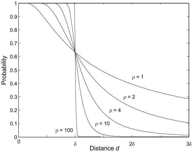
With our choice of transmission kernel the expression 1 − p(d), the probability that one infectious animal will infect one susceptible animal a distance d away in one day, is monotonically decreasing from 1 to 0 as d increases (Fig. 1). Notice that δ is a distance-scaling factor; specifically, it is the distance at which the probability is 1−1/e (or about 63%) that one infectious animal will infect one susceptible animal in one day. The ρ parameter determines whether the decay from 1 to 0 is gradual (small ρ) or step-like (large ρ). Notice that as ρ increases this stochastic model becomes more deterministic in that for very large values of ρ a susceptible animal is almost certainly infected in one day if it is within distance δ of an infectious animal, and is almost certainly not infected otherwise.

Fig. 1.

The probability that one infectious animal will infect one susceptible animal a distance δ units away in one day for various values of the parameter ρ.

In this paper we shall assume that our epidemic parameters do not change over the course of the epidemic. There are cases when this is not a reasonable assumption, such as in a community in which an epidemic’s duration spans both a dry season and a wet season during which the transmission characteristics of the virus can be expected to be different. The methods in this paper can be generalized to accommodate such a change in parameter values, although at the expense of less accuracy since more parameter values must be determined.

With our choice of kernel, Eq. (1) becomes

$$P_{jk}(\delta ,\rho )=1-\prod _{i\in A(k)}exp\left(-N_i{N}_j{\left(\frac{\delta }{d_{ij}}\right)}^{\rho }\right)$$ (4)

Given the geographic information about the farm community (the coordinates of the farms and the number of animals on each), the index farm of an epidemic (the first farm infected), and the values of the epidemic parameters (δ and ρ), we may generate a stochastic simulation of an epidemic day by day based on Eq. (4). By running a large number of simulated epidemics we may estimate many properties of an ongoing epidemic, such as its expected attack rate and its expected duration.

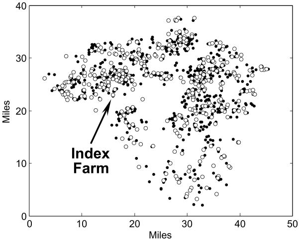
We implemented our LND model in a hypothetical poultry farm community located in Lancaster County, Pennsylvania (USA). The map of farm locations and data concerning the number of birds in each of the premises in Lancaster County were abstracted from a synthetic national map of poultry farms with the same marginal properties as the county-scale data available in the 2002 U.S. Census of Agriculture (Bruhn et al., 2007). We resorted to synthetic data because the actual locations of poultry premises in Lancaster and many other counties in the USA are not available in the public domain. Figure 2 is the map of the synthetic farm community used throughout this paper.

Fig. 2.

Synthetic map of 946 poultry farms in Lancaster County, Pennsylvania containing almost 23 million birds. The black disks identify 578 small farms (<400 birds) containing 0.5% of all birds and the white disks identify the remaining 368 farms containing 99.5% of all birds. The arrow points to farm #663 used as the index farm in our simulations.

Figure 3 displays the attack rates of 21,000 simulated epidemics with index farm 663 and epidemic parameters δ* = 3×10⁻⁶ and ρ^* = 2. These epidemic parameters were chosen because they yielded simulated epidemics with characteristics similar to an actual poultry epidemic in Lancaster County. More specifically, we generated day-by-day geographical movies of simulated epidemics for many epidemic parameters and compared them with the actual day-by-day epidemic movie and tried to match as many features as possible, such as attack rate, duration of the epidemic, temporal peak of the epidemic, distribution of infected farms, and so forth.

Fig. 3.

The attack rates of 21,000 ordered simulated epidemics with farm #663 as the index farm and epidemic parameters δ* = 3×10⁻⁶ and ρ^* = 2. There were 14,443 ‘mild’ simulations (epidemics with early stochastic extinction for which 5 or fewer farms out of 946 were infected) and 6557 ‘severe’ epidemics (all with 276 or more infected farms). The jump is at 0.6878 and the mean of the attack rate for the severe epidemics is 0.30. The inset map is a histogram of the 6557 severe epidemics.

The horizontal axis in Fig. 3 is the fraction of simulations in increasing order of their attack rates and the inset map is the histogram of the attack rates for the 6557 severe epidemics, which we define as those epidemics in which more than one percent of the farms were infected (>9 farms or an attack rate > 0.01). As Fig. 3 shows, the attack rate jumps from 0.0053 to 0.2706 (a factor of 51) at the 68.8% level. The step pattern evident in Fig. 3 is typical of all index farms in this community. That is, for each index farm a certain fraction of the epidemics will be mild and the remaining will be severe with a rather fixed mean attack rate and rather small variance. However, the fraction of the epidemics that are severe varies significantly from one index farm to another. Some index farms (e.g., small farms remote from other farms) will have a very small fraction of severe epidemic so that the location of the jump in Fig. 3 will be close to one along the horizontal axis. But for some large index farms located close to many other farms almost all epidemics will be severe, and so the location of the jump will to close to zero. Our simulations, however, show that all severe epidemics, regardless of which farm was the index farm, are quite similar as to their attack rates and which farms are ultimately infected. In other words, what changes in Fig. 3 from one index farm to another is the location of the jump in the curve along the horizontal axis, but the magnitude of the jump and in the inset histogram are approximately the same for all index farms.

As the epidemic parameters vary, Fig. 3 changes quantitatively, but not qualitatively. The step pattern persists, but for any fixed index farm a change of epidemic parameters results in a change in the location and the height of the jump. Some epidemic-parameter values lead to severe epidemics with very high attack rates (although relatively constant over all index farms) while other values lead to severe epidemics with low attack rates.

In generating target epidemics from which to obtain estimates, only severe epidemics were used. Mild epidemics were not considered for target epidemics because there were not enough infected farms to obtain good estimates with our methods. All of the mild epidemics we generated resulted in fewer than six infected farms, and working with so few cases is somewhat equivalent to trying to determine whether a coin is fair by tossing it fewer than six times.

First Pair of Estimators (Method 1)

Of the three estimators we developed, this first one is the most precise. It is a maximum likelihood estimator dependent on having an expression for the probability that an infectious animal will infect a susceptible animal a specified distance away in one day. It requires a knowledge of which premises were infectious on a set of days and which susceptible premises became infected on those days.

For a given epidemic let B(i) and C(i) be the sets of indices of the susceptible farms that were and were not infected on the i^th day of the epidemic, respectively. Next, let A= {a₁, a₂, …, a_K} be the set of indices of K days of the epidemic on which data were collected as to which susceptible farms were and were not infected on that day. Then the probability of the observed pattern over the K days, based on our probabilistic model of the spread of the epidemic, is

$$L_{1A}(\delta ,\rho )=\prod _{k=1}^K\left\{\left[\prod _{j\in B(a_k)}\left(1-P_{{ja}_k}(\delta ,\rho )\right)\right]\left[\prod _{j\in C(a_k)}{P}_{j{a}_k}(\delta ,\rho )\right]\right\}$$ (5)

This expression is a product that has as many factors as the cumulative number of susceptible farms at the beginnings of the K days for which data were collected.

Equation (5) defines the maximum likelihood function for δ and ρ. By definition, the maximum likelihood estimates for δ and ρ are those values that maximize L_1A(δ, ρ); that is, those values the make the observed epidemic the most likely.

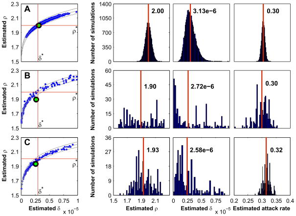
Figure 4(A) illustrates the results for 28,713 estimates of δ and ρ using the farm community in Fig. 2 and target values of δ* = 3×10⁻⁶ and ρ^* = 2. The days on which the required data were collected were assumed to be all of the days of the epidemic. To generate this figure, 100 target epidemics were run using each of the 946 farms as the index farm, a total of 94,600 target epidemics. Then the mild epidemics were discarded and the maximum likelihood estimates for δ and ρ for the remaining 28,713 severe epidemics were determined by maximizing L_1A(δ, ρ) over all δ and ρ. The mild epidemics were discarded because for those fewer than 10 farms were infected (by definition) which was too few to obtain good estimates. The resulting scatter diagram for δ and ρ is displayed together with their individual histograms on the top row. The histogram of the attack rates of the severe epidemics is displayed in the last column of the top row. The 95% confidence intervals for these three quantities were evaluated by determining the intervals in which the middle 95% of the corresponding values lie. For δ this interval was [1.67, 5.21] ×10⁻⁶, for ρ it was [1.92, 2.09], and for the attack rate it was [0.292, 0.316].

Fig. 4.

Scatter diagrams and histograms for the three estimator methods. The target values for all three cases are δ* = 3×10⁻⁶ and ρ^* = 2. In the scatter diagrams the green dots are the sample means and the three curves are lines along which the expected severe attack rate is constant. In the histograms the vertical red lines indicate the sample means. (A) Method 1, (B) Method 2, (C) Method 3.

The expected attack rate of a severe epidemic is a function of the index farm and the two epidemic parameters. For a fixed index farm and fixed epidemic parameters this expected value can be approximated by taking the sample mean of the attack rates of a large number of simulated severe epidemics. Level curves for the expected severe attack rate can then be determined numerically as a function of δ and ρ for a fixed index farm. Figure 4(A) shows three such level curves of the expected severe attack rate of index farm 663 as a function of δ and ρ. These level curves were computed by running 100 simulated severe epidemics with farm 663 as the index farm for each value of δ and ρ in a fine mesh in the δρ-plane and taking the mean of the 100 resulting attack rates at each mesh point.

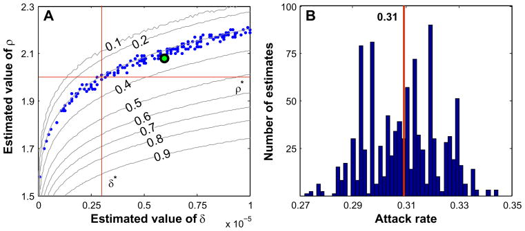
These level curves varied very little for different index farms, indicating that the expected severe attack rate depends more on the geometry of the farm community than on which farm the epidemic began. Figure 8(A) displays the level curves corresponding to severe attack rates of 0.1, 0.2, …, 0.9 for our farm community. We also verified this insensitivity of the level curves to the index farm with a different farm community of about 4200 poultry farms that approximated the true distribution of poultry farms in Pennsylvania within a 100-mile radius of Lancaster, Pennsylvania. We plotted the level curves corresponding to values of the severe attack rates equal to 0.1, 0.2. 0.3, 0.4, 0.5, 0.6, and 0.7 for ten index farms chosen at random. The level curves matched almost pixel-for-pixel on a computer monitor for the ten index farms.

Fig. 8.

(A) Scatter diagram of 1000 estimates of δ* = 3×10⁻⁶ and ρ^* = 2 using Method 3 with 1000 random choices of half of the farms. The curves are lines of constant severe attack rate labeled with their corresponding values. Most of the estimates lie along the curve corresponding to the severe attack rate of 0.3. The green dot is the sample mean of the 1000 estimates. (B) Histogram of 1000 estimates for the severe attack rate of a target epidemic using the estimated epidemic parameters in (A). The target attack rate was 0.30 and the sample mean of the 1000 estimates was 0.31.

Regardless of which farm was used as the index farm for a target epidemic, its corresponding estimates for δ and ρ lay along an arc of values evident in the scatter diagram. This arc identifies a valley in the surface diagram of the likelihood function L_1A (δ, ρ) as a function of its arguments for all target epidemics that we ran. What changed with each target epidemic was the location of the minimum within the common valley. This common valley, in fact, lies along a typical level curve of the estimated severe attack rate as a function of δ and ρ; specifically, the typical contour passing through the target values δ* and ρ^* for any index farm.

Moreover, the fact that all of our estimates for δ and ρ are distributed near one of these contour lines indicates that we can obtain a fairly consistent estimate for the attack rate of a particular epidemic from the various estimates, as is verified by the 95% confidence interval for the attack rate.

Notice from the histogram for ρ that its maximum likelihood estimator is unbiased; that is, its expected value is equal to the target value. The estimator for δ, however, has a bias of about +5%.

While Fig. 4(A) was for estimated values obtained after an epidemic was over, we also applied the procedure for the case where data are collected on a daily basis, so that K in Eq. (2) ran from 1 to the number of days in the epidemic. As an example, for one particular 118-day simulated target epidemic with an attack rate of 0.3044: on day 19 the estimated attack rate was 0.24 to two decimal places; on days 30 and 40 it was 0.27 and 0.28, respectively; and from day 50 until day 118 it was 0.30 to two decimal places. This example was typical in that early estimates for the attack rate were low and then gradually increased to the actual value, arriving at excellent approximations well before the peak of the epidemic.

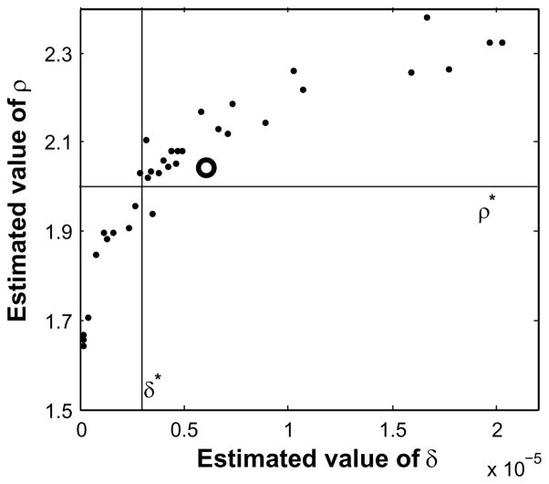
Although this estimator needs much detailed data, it is possible that the data even for one day is enough to get good estimates for δ and ρ. For example, if on one day there are 800 susceptible farms and 50 infectious farms, we have 800 bits of data; namely, which susceptible farms did and did not become infected on that day. If there was a good mix of infected and non-infected susceptible farms on that day, these 800 bits of data would be enough to determine the two epidemic parameters fairly well, assuming the maximum likelihood assumption that the observed epidemic was typical. We tested this hypothesis on one of the epidemics used in Fig. 3. We picked 34 of the 109 days of the epidemic that had a good mix of infected and non-infected susceptible farms and generated 34 estimates for the epidemic parameters. These are displayed in Fig. 5. The sample mean of these 34 estimates is δ_mean = 6.03×10⁻⁶ and ρ_mean = 2.4 with a good distribution of estimates about the target values. Although there is a fair amount of variance in the estimates for target values δ^* and ρ^*, they all lie fairly close to the level curve for the severe attack rate of the target epidemic. Consequently, one day’s complete data on a fairly active day of the epidemic is enough to obtain a good estimate of the attack rate of a severe epidemic. Such an estimate would be extremely useful in controlling an epidemic.

Fig. 5.

Scatter diagrams of 34 pairs of estimates of the epidemic parameters using Method 1 for a single target epidemic with δ* = 3×10⁻⁶ and ρ^* = 2. Each pair of estimates used the data for one of the 109 days of the epidemic. The white circle identifies the mean of the 34 estimates: δ_mean = 6.03×10⁻⁶ and ρ_mean = 2.4.

The results presented in Fig. 4 are for the target epidemic parameters δ* = 3×10⁻⁶ and ρ^* = 2. We obtained similar results when choosing target parameters chosen at random with δ* in the interval [0, 10⁻⁵] and ρ^* in the interval [1.5, 3.0]. Specifically, we chose random pairs of values uniformly from those intervals and kept the first ten pairs for which the fraction of severe epidemics was greater than 0.02 (cf., Fig. 3 for which the fraction of severe epidemics was 0.31). For these ten pairs of target parameters we determined 100 estimates for them based on 100 simulated target epidemics. All ten pairs yielded diagrams similar to those in Fig. 4, but with differing amounts of bias in the sample means of the estimated target epidemics.

Second Pair of Estimators (Method 2)

Although the maximum likelihood estimators of Method 1 give excellent results, they require more data about an ongoing or past epidemic than are usually available. More typically, we have at hand daily or weekly reports of the number of newly detected infectious premises without any precise information on their location. We can compare the actual number of newly infectious farms for many different days with the expected number for a given set of epidemic parameters and choose those values of the epidemic parameters that minimize this difference in some sense. We quantitatively measured this difference in the form of an error function, which we take as the cumulative variation between the predicted and actual number of newly infectious farms on those days for which we collected data. Specifically, this error function is given by

$$L_{2j}(\delta ,\rho )=\sum _{k=1}^K|Q_{a_k}-F_{j{a}_k}(\delta ,\rho )|$$ (6)

where {a₁, a₂, …, a_K} is a set of indices of K days on which data were collected, Q_k is the number of newly infectious farms on the k^th day, and F_jk(δ,ρ) is the expected number of newly infectious farms on the k^th day of a severe epidemic when the j^th farm is the index farm. We approximated the value of F_jk(δ,ρ) by taking the mean of the number of newly infectious farms on the k^th day of a large number of simulated severe epidemics (about 100) using the j^th farm as the index farm and the indicated values of δ and ρ. Only severe epidemics were used to approximate F_jk(δ,ρ) because the target epidemic was severe. Our estimators for δ and ρ are those values of δ and ρ that minimize this error function.

Figure 4(B) shows the scatter diagram and histograms for 287 estimates based on the same number of severe target epidemics, each with the same index farm (farm 663) and the same target values of δ * = 3×10⁻⁶ and ρ^* = 2. The sum is taken over the entire course of the epidemic so that K is the number of days in the epidemic. As with Method 1, the estimates are distributed about the level curve of the severe attack rate through the target values. The histograms, however, do not have the nice Gaussian shape as do those of Method 1, and both estimators are biased slightly below the target values.

Notice that the histogram for δ in Fig. 4(B) shows many estimates much smaller that the target value δ *. In particular, the smallest bin in the histogram contains many estimates at least an order of magnitude smaller than the target value, although none of them is actually zero.

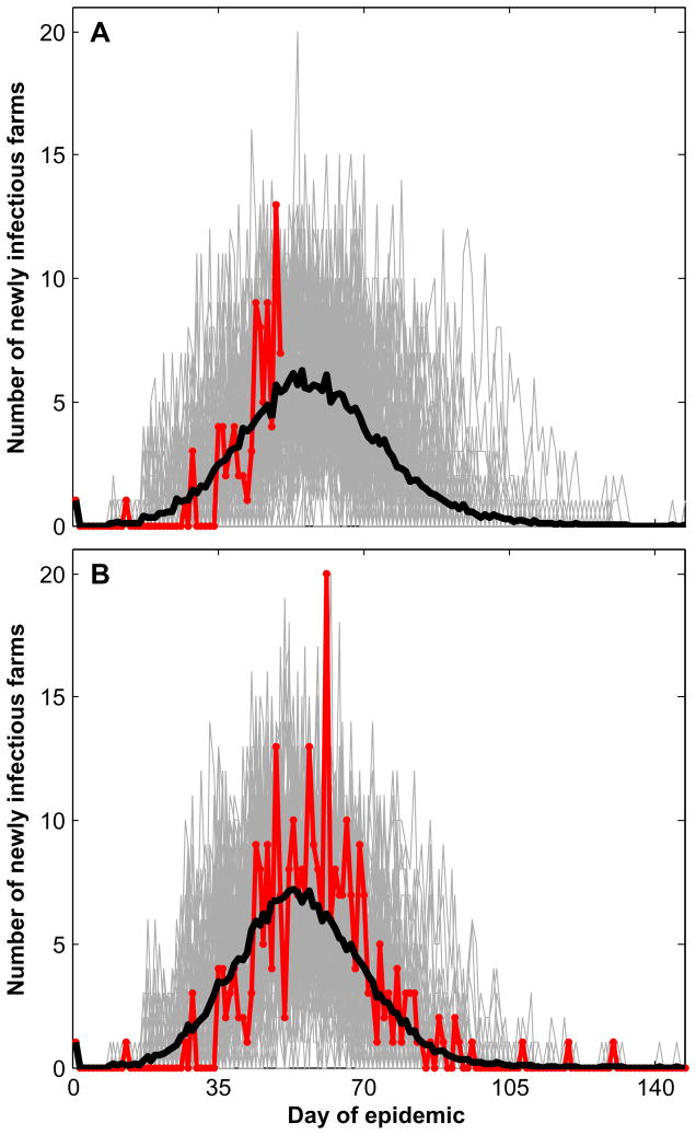
Figure 6 shows how Method 2 works when applied in a progressive daily manner. The red curve in Fig. 6(A) displays the daily number of newly infectious cases up to day 50 of a target epidemic having index farm 663; the gray curves are the analogous curves for 100 severe epidemic simulations using the estimated values of δ and ρ obtained by minimizing Eq. (4) with K=50 and j=663; and the black curve is the daily average of the 100 gray curves. The black curve predicts an attack rate of 0.256. Figure 6(B) is the corresponding set of curves at the end of the epidemic (K=147). The actual attack rate was 0.310 and the attack rate predicted by day 147 was 0.279.

Fig. 6.

(A) The actual daily number of exposed farms of a target epidemic up to day 50 is shown in red. The estimated daily number based on this 50-day data set is shown by the black curve, which is the daily mean of the 100 simulated curves shown in gray. (B) The actual daily number of exposed farms for the complete epidemic of 147 days is shown In red. The estimated daily number based on this 147-day data set is shown by the black curve, which is the daily mean of the 100 simulated curves shown in gray.

Third Pair of Estimators (Method 3)

The scenario for our third pair of estimators for the epidemic parameters is that we know which farm was the index farm of a severe epidemic and which farms were infected or not infected up to a certain day, although we do not know when they became infected. A typical example of the use of this error function is when archival data are available for a completed epidemic as to which farms in a community were or were not infected during the epidemic.

We constructed an error function that is a measure of the difference between the pattern of actual farms infected and the probable farms infected and took as our estimators for δ and ρ those values that minimize this difference. To describe our method, set B_ik equal to one if the i^th farm had been infected up to and including the k^th day of the observed epidemic in which the j^th farm was the index farm and set B_ik equal to zero otherwise. We then define the following error function:

$$L_{3jk}(\delta ,\rho )=\sum _{i=1}^N|B_{ik}-I_{\mathit{ijk}}(\delta ,\rho )|$$ (7)

where N is the number of farms in the community and I_ijk(δ,ρ) is the probability that the i^th farm will be infected up to and including the k^th day of a severe epidemic in which the j^th farm was the index farm. We approximated the value of I_ijk(δ,ρ) by the fraction of times that the i^th farm was infected up to and including the k^th day for a large number of simulated sever epidemics (about 100) using the j^th index farm and the indicated values of δ and ρ. Our estimators for δ and ρ are those values of δ and ρ that minimize this error function.

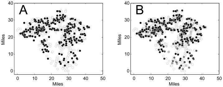
Figure 7 illustrates the idea behind our error function. In Fig. 7(A) the farms in a simulated target epidemic in Lancaster County that were infected during the course of the epidemic are shown by black disks and those not infected are shown by white disks (farm 663 was the index farm). In Fig. 7(B) each farm is colored a shade of gray corresponding to the probability of the farm being infected for the values of δ and ρ that minimize the error function in Eq. (7). This grayscale image is the closest approximation to the black-and-white image according to our error function and determines the estimators for the epidemic parameters using our Method 3.

Fig. 7.

(A) The farms that were infected in a target epidemic are in black and those not infected are in white. (B) Each farm is colored a shade of gray according to its probability of being infected. The two epidemic parameters used are the ones that minimize the error function in Eq. (7).

Suppose a total of M simulations are used to estimate the expected value I_ijk(δ,ρ) and that J_ijkm(δ,ρ) is one if in the m^th simulation the i^th farm is infected by the k^th day and zero otherwise. Then

$$I_{\mathit{ijk}}(\delta ,\rho )=\frac{1}{M}\sum _{m=1}^M{J}_{\mathit{ijkm}}(\delta ,\rho )$$ (8)

and Eq. (7) can be expressed as

$$L_{3jk}(\delta ,\rho )=\frac{1}{M}\sum _{m=1}^M\left[\sum _{i=1}^N|B_{ik}-J_{\mathit{ijkm}}(\delta ,\rho )|\right]$$ (9)

The inner sum in Eq. (9) is the number of farms in the m^th simulation that did not match up with farms in the target epidemic as to having been or not been infected by the k^th day. The outer sum is the average of this number of misses over the M simulations and consequently is an approximation to the expected number of misses if the number of simulations is large. Our error function for Method 3 thus determines the values of δ and ρ that minimize the expected number of misses.

Figure 4(C) shows the scatter diagram and histograms of 287 estimated values of δ and ρ generated from the same number of simulated severe epidemics with farm 663 as the index farm. The target epidemic parameter values were δ* = 3×10⁻⁶ and ρ^* = 2 and K was equal to the number of days of the epidemic. The results are similar to those of Method 2; namely, the estimates are under-biased and fall along the contour line of the attack rate corresponding to the target values of the epidemic parameters and index farm.

We may modify the scenario for this third method by supposing that we have infection data for only some of the farms in the community after an epidemic. For example, we may have archival data of an epidemic in which we know which farms were infected in a region of the farm community encompassing only about half of the farms in the community. In this case, we replace the sum in Eq. (7) over all of the farms by the sum over those farms for which we have data. However, the farms that are known to have been infected should be representative of the farm community as a whole and ideally should be a random sample of all of the farms.

Figure 8 is an example when we have data for only half of the farms in our synthetic RTI community. We first simulated a severe target epidemic with index farm 663 and epidemic parameters δ* = 3×10⁻⁶ and ρ^* = 2; chose half of the farms at random; computed the estimates for δ and ρ by minimizing Eq. (7); and then determined the expected attack rate corresponding to the estimated values by taking the mean of the attack rate of 1000 simulated severe epidemics generated using the estimated values of δ and ρ. This was repeated 1000 times (throwing away 6 cases for which our minimization algorithm failed) and the results were plotted in Fig. 8. The mean of the 1000 estimates for the attack rate is 0.31 and the actual attack rate of the control epidemic was 0.30. This compares with an estimated attack rate of 0.32 when using the data from all of the farms in the community.

Summary

Our desire in this research was to develop an arsenal of estimation techniques for the epidemic parameters that quantify a mathematical model of an animal epidemic. It is essential to have accurate models in order to design effective vaccination policies to prevent future epidemics or to implement effective culling policies to control ongoing epidemics. Our upcoming research objectives include determining how much error is tolerable in the estimation of these parameters in order to design effective vaccination and culling policies.

All three of our estimation methods required knowing the locations of the premises in the farm community and the numbers of animals on each premises. However, the implementation of each of the three methods required different data about a target epidemic. Method 1 required knowing which farms were infectious on specific days of the epidemic and which susceptible farms did and did not become infected on those days. Method 2 required knowing how many farms, but not which farms, became infected on specific days. Finally, Method 3 required knowing which farms were infected up to a specified day (possibly the last day) of an epidemic, but did not require knowing on which day each farm became infected.

When our target epidemic was generated using the assumed mathematical model with specific target epidemic parameters, we had complete knowledge of which farms were infected and when each was infected. Consequently, we could run all three of our methods independently under a variety of conditions. As our results in this paper show, all three methods gave consistent and good estimates for the target epidemic parameters.

The way in which the estimated values for δ and ρ for all three methods all lie roughly along the same contour of constant attack rate is particularly interesting (first column of Fig. 4). It shows that the estimates for these two parameters are strongly correlated for a fixed farm community and that this correlation is governed by the expected attack rate determined by the target values of δ and ρ.

Of course, the estimation techniques we developed require that the underlying mathematical model describe the actual epidemic reasonably well. If this is not the case, then the estimation technique can be expected to fail, which would itself be an indication that the underlying model is faulty.

The computational effort associated with Method 1 was not excessive, even for farm communities much larger than the one we used in this paper. However, Methods 2 and 3 require the generation of millions of epidemic simulations to implement. Typical computation time for one phase of estimating our two parameters using data from a single epidemic was about 7 hours for our 946-farm community on a 4-core, 2.4 gigahertz computer with 4 gigabytes of RAM running Windows Vista. For a farm community with 4235 farms, the computation time was about 23 hours on an 8-core, 2.7-gigahertz computer with 32 gigabytes of RAM running RedHat Linux.

Parameter estimates are essential in running good simulations of an ongoing epidemic. We are now in the process of gathering data from actual epidemics to test our estimation techniques. We are particularly interested in past epidemics for which there is enough data to apply all three methods. If, then, all three methods yield similar parameter estimations, this would be an excellent indication that the underlying model is valid.

References

- Bruhn M, Cajka J, Smith G, Curry R, Dunipace S, Wheaton W, Cooley P, Wagener D. Generating Realistic Livestock and Poultry Operations to Support Development of Infectious Disease Control Strategies. Proceedings of the ESRI Health GIS Conference; October 7th–10th, 2007; Scottsdale AZ. 2007. pp. 1–13. [Google Scholar]
- Chowell G, Rivas AL, Hengartner NW, Hyman JM, Castillo-Chavez C. The Role of Spatial Mixing in the Spread of Foot-and-Mouth Disease. Preventive Veterinary Medicine. 2006;73:297–314. doi: 10.1016/j.prevetmed.2005.10.002. [DOI] [PubMed] [Google Scholar]
- Erlander S, Stewart NF. The Gravity Model in Transportation Analysis - Theory and Extensions: Topics in Transportation. VSP; Utrecht: 1990. [Google Scholar]
- Falcon MD. Exotic Newcastle disease. Seminars in Avian and Exotic Pet Medicine. 2004;13:2, 79–85. [Google Scholar]
- Ferguson NM, Donnelly CA, Anderson RM. The Foot-and-Mouth Epidemic in Great Britain: Pattern of Spread and Impact of Interventions. Science. 2001;292:1155–1160. doi: 10.1126/science.1061020. [DOI] [PubMed] [Google Scholar]
- Keeling MJ. Models of Foot and Mouth Disease. Proc R Soc B. 2005;272:1195–1202. doi: 10.1098/rspb.2004.3046. [DOI] [PMC free article] [PubMed] [Google Scholar]
- Keeling MJ, Woolhouse ME, Shaw DJ, Matthews L, Chase-Topping M, Haydon DT, Cornell SJ, Kappey J, Wilesmith J, Grenfell BT. Dynamics of the 2001 UK foot and mouth epidemic: stochastic dispersal in a heterogeneous landscape. Science. 2001;294:813–817. doi: 10.1126/science.1065973. [DOI] [PubMed] [Google Scholar]
- Keeling MJ, Woolhouse MEJ, May RM, Davies G, Grenfell BT. Modeling vaccination strategies against foot and mouth disease. Nature. 2003;421:136–142. doi: 10.1038/nature01343. [DOI] [PubMed] [Google Scholar]
- Keeling MJ, Eames KTD. Networks and epidemic models. J R Soc Interface. 2005;2:295–307. doi: 10.1098/rsif.2005.0051. [DOI] [PMC free article] [PubMed] [Google Scholar]
- Kinde H, Utterback W, Takeshita K, McFarland M. Survival of exotic Newcastle disease virus in commercial poultry environment following removal of infected chickens. Avian Diseases. 2004;48:3, 669–674. doi: 10.1637/7161-020104R. [DOI] [PubMed] [Google Scholar]
- Tildesley MJ, Savill NJ, Shaw DJ, Deardon R, Brooks SP, Woolhouse MEJ, Grenfell BT, Keeling MJ. Optimal reactive vaccination strategies for a foot-and-mouth outbreak in the UK. Nature. 2006;440:83–86. doi: 10.1038/nature04324. [DOI] [PubMed] [Google Scholar]
- Tildesley MJ, Keeling MJ. Modelling Foot and Mouth Disease: a comparison between the UK and Denmark. Preventive Veterinary Medicine. 2008;85:107–124. doi: 10.1016/j.prevetmed.2008.01.008. [DOI] [PubMed] [Google Scholar]
- Toma B, et al.1999Dictionary of Veterinary Epidemiology Iowa State University Press; Ames [Google Scholar]