Measurement of cortical thickness from MRI by minimum line integrals on soft‐classified tissue

Abstract

Estimating the thickness of the cerebral cortex is a key step in many brain imaging studies, revealing valuable information on development or disease progression. In this work, we present a framework for measuring the cortical thickness, based on minimizing line integrals over the probability map of the gray matter in the MRI volume. We first prepare a probability map that contains the probability of each voxel belonging to the gray matter. Then, the thickness is basically defined for each voxel as the minimum line integral of the probability map on line segments centered at the point of interest. In contrast to our approach, previous methods often perform a binary‐valued hard segmentation of the gray matter before measuring the cortical thickness. Because of image noise and partial volume effects, such a hard classification ignores the underlying tissue class probabilities assigned to each voxel, discarding potentially useful information. We describe our proposed method and demonstrate its performance on both artificial volumes and real 3D brain MRI data from subjects with Alzheimer's disease and healthy individuals. Hum Brain Mapp 2009. © 2009 Wiley‐Liss, Inc.

INTRODUCTION

Measuring the cortical thickness has long been a topic of interest for neuroscientists. Cortical thickness changes in a characteristic pattern during childhood development and with the progression of neurodegenerative diseases such as Alzheimer's, HIV/AIDS, and epilepsy [Thompson et al.,2004,2005]. Recent studies examining changes in cortical thickness over time have revealed the trajectory of diseases in the living brain, and have been used to quantify treatment effects, identifying regions where cortical thickness correlates with age, cognitive deterioration, genotype, or medication.

Various approaches have recently been proposed to automate this cortical thickness measurement from magnetic resonance imaging (MRI) data, e.g. (Thorstensen et al., unpublished), [Fischl and Dale,2000; Jones et al.,2000; Kabani et al.,2001; Lerch and Evans,2005; Lohmann et al.,2003; Yezzi and Prince,2003; Young and Schuff,2008]. The limited spatial resolution of most MRI volumes (typically 1–2 mm) makes it difficult to measure cortical thickness accurately, as it varies from 2 to 5 mm in different brain regions and is only a few voxels thick in the images. The neuroscience community has not yet agreed on a unique definition of cortical thickness and so far the various methods proposed measure slightly different quantities. What is common among them is that they virtually all perform a pre‐segmentation of the white matter (WM), gray matter (GM), and cerebrospinal fluid (CSF), and most extract explicit models of the surfaces between them (i.e., the inner surface between WM and GM and outer surface between GM and CSF). They then use this hard segmentation as the input data for different tissue thickness measurement algorithms (“Previous Related Work” section briefly reviews previous work and comments more on this). The disadvantage of this approach is that in the hard segmentation process, information is discarded and decisions are made before measuring the tissue thickness, a significant local error in measured thickness could be introduced by a few misclassified voxels (see the “Artificial Data” section for an example).

The approach we adopt here uses a soft prelabeled/classified volume as the input data, keeping valuable information all the way into the step of measuring tissue thickness. Because of the limited resolution of an MRI volume, many voxels contain partial amounts of two or more tissue types [see Pham and Bazin,2004 and the references therein]. Their intensity values give us information about the probability or proportion of those voxels belonging to any of the categories of WM, GM, or CSF. Rather than a (hard) preclassified volume, we use one containing the probability that each voxel belongs to the GM.1 These probability values have the same precision as the values in the original MRI volume, and therefore we do not discard any useful information.2 We compute line integrals of the soft classified data, centered at each voxel and in all possible spatial directions, and then consider their minimum as the local cortical thickness at that voxel.

While hard segmentations are often used as part of the analysis, e.g., to warp surfaces for population studies and/or for visualization, many useful statistics can be performed completely avoiding this hard classification, e.g., region‐based statistics. Moreover, volumetric warping avoids hard segmentation. Even if hard segmentation is to be performed for other parts of the analysis, the errors produced by it need not to be transferred to the tissue thickness computation. This error transfer is common in the techniques mentioned below and avoided with our proposed framework.

In the “Previous Related Work” section, we review previous work on cortical thickness measurement. The “Methods” section describes our proposed framework, and experimental results are presented in the “Results and Discussion” section. The “Conclusion” section concludes with a review of the contributions, and finally the implementation is covered in detail in the Appendix.

An early conference version of this work was published in [Aganj et al.,2008]. Here, we extend this work with more validation and comparisons. In addition, the implementation of the algorithm is provided in detail, and a new technique to find the GM skeleton is introduced.

PREVIOUS RELATED WORK

We now discuss some of the previously reported work for measuring the cortical thickness. While many additional very important works have been published, those mentioned below provide a good representation of the spectrum of techniques available in the literature. Most methods require a (hard) pre‐segmentation of the inner and outer surface, which results in a loss of available information and often inaccuracy in the input for the main thickness measurement algorithm. This loss, while manifested at different levels depending on the sophistication of the algorithm, is intrinsic to all hard segmentation methods.

Coupled‐surface methods [Fischl and Dale,2000; MacDonald et al.,2000] define the cortical thickness as the Euclidean distance between corresponding point pairs on the inner and outer surfaces, often with parametric grids imposed. A displaced surface may result in an overestimation of the thickness (see Fig. 1a). Closest point methods such as [Miller et al.,2000] compute for each point on one of the two surfaces the closest point on the other surface and define the thickness as the Euclidean distance between them. The main drawback with these methods is the absence of symmetry, as seen in Figure 1b. In another method introduced in [Scott and Thacker,2004], the regional histogram of thickness is estimated by measuring the length of the line segments connecting the inner and outer surfaces of the GM layer, normal to one of the surfaces. The median of the histogram is then chosen as the local cortical thickness. A detection of the WM‐GM and GM‐CSF boundaries is however necessary.

Figure 1.

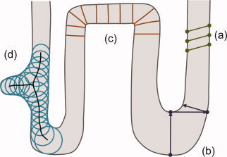
Common ways of measuring cortical thickness. (a) Coupled‐surface methods. (b) Closest point methods. (c) Laplace (“heat‐flow”) methods. (d) Largest enclosed sphere methods. [Color figure can be viewed in the online issue, which is available at www.interscience.wiley.com.]

Laplace methods [Haidar and Soul,2006; Jones et al.,2000; Yezzi and Prince,2003] solve Laplace's equation in the GM region with the boundary condition of constant (but different) potentials on each of the two surfaces. The cortical thickness is then defined at each point as the length of the integral curve of the gradient field passing through that point, as illustrated in Figure 1c. With this approach, the thickness is uniquely defined at every point. Nevertheless, a presegmentation of the two surfaces is required, reducing the accuracy of this technique.

Another category of methods defines thickness by making use of a central axis or skeleton (Thorstensen et al., unpublished) [Pizer et al.,1998]. Thickness is typically estimated as the diameter of the largest enclosed sphere in the GM layer, which is (in some cases only initially) centered on a point on the central axis. As Figure 1d demonstrates, a relatively sharp change in the thickness may result in a new branch and affect the topology of the skeleton.

The vast majority of the methods reported in the literature propagate segmentation errors to later steps, and segmentation is still in itself a challenging problem in brain imaging. Considering that the GM layer spans only a few voxels at the commonly used 1–2 mm resolutions, these errors can be significant, and measuring tissue thickness avoiding this hard segmentation step may be very beneficial. This is the approach introduced here and described next.

METHODS

Definition

In its simplest form, we define the thickness of the GM at a given voxel as the minimum line integral of the probability map of the GM over all lines passing through that voxel.3 Formally:

where is the thickness of the GM at a point , is the probability of the point belonging to the GM (estimation of this probability is described in Appendix), and is the set of all lines in three‐dimensional space passing through the point . In practice, however, is comprised of all equal‐length line segments centered at , which are sufficiently longer than the expected maximum thickness in the volume. Choosing longer line segments does not greatly affect the integral values since decreases significantly on the non‐GM regions.4 Figure 2a shows an example of this construction, for a 2D binary probability map, where the probability of belonging to the GM is 1 inside the shape and 0 outside. When computing thickness at the specified point, the line segment marked with oval arrows is selected as the one giving the smallest line integral. The corresponding integral value, which in this case is the length of its overlap with the GM (in bold), is the thickness of the GM at that point. A more realistic situation is shown in Figure 2b, where the probability map varies between zero and one. A blurred border, which results from the limited resolution of the MRI, includes voxels that partially contain GM. Because of the pre‐segmentation, this type of partial volume information is not considered in most prior work in this area.5

Figure 2.

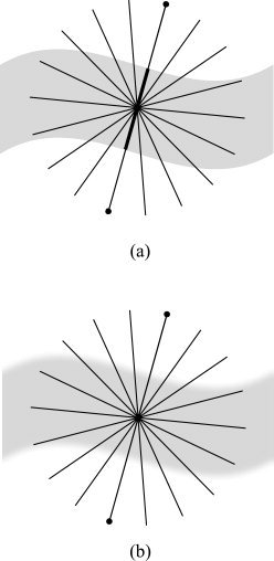
Computing line integrals passing through a point, and choosing the minimum integral value as the thickness. (a) Binary probability map. (b) Continuous probability map.

Our method is based on an intuitive way of measuring the thickness of an object. A simple way to measure the local thickness of an object would be to put two fingers on both edges of the object, and move the finger tips locally (equivalent to varying the angle of the segment connecting them to each other), until the Euclidean distance between them is minimized (see Fig. 3). For example, among Figure 3a–c, we would naturally choose Figure 3b as the one that depicts the most accurate local thickness. This distance could then be considered as the local thickness of the object. Thus, we are dealing with a constrained optimization problem: minimizing a distance in a specific region. In our approach, however, this region is identified precisely by the point where we want to define the thickness. Therefore, the constraint is that the point must be on the line segment connecting the two finger tips. In other words, we consider only the line segments passing through the point where we intend to find the thickness. The minimized distance—or the length of the line segment—is in this case the integral of the probability map on the line containing the segment (Fig. 3e).

Figure 3.

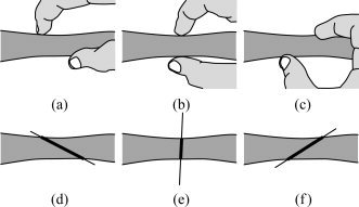
(a–c) An intuitive way of measuring the thickness of an object. (d–f) Our algorithm produces results similar to this intuitive approach.

Algorithm

The algorithm basically computes every line integral centered at each point of the volume starting from the point of interest and proceeding in each of the two opposite directions separately (see Appendix for our discretization method). Once all the line integrals at a point are calculated (meaning in all possible directions), the minimum of them is considered to be the thickness at that point. However, to reduce the effect of noise, an alternative would be for instance to consider the average of some of the smallest integrals.

In practice, a problem may arise, typically in narrow sulci where the outer surface of the folded GM layer has two nearby sides (Fig. 4a). While computing the thickness on one part of the layer, the GM of the other part may be partially included in some of the line integrals; this will lead to the thickness being overestimated (Fig. 4b). To avoid this error, we include two stopping criteria, which prevent a line integral from further advancing when it is believed that no more summation is necessary or that we are mistakenly considering a different region of the GM layer. The line integral stops proceeding if the probability map:

• 1Has been below a specific threshold for a certain number of consecutive voxels, or
• 2Has been decreasing at least for a certain number of successive voxels and then increasing for an additional number of voxels.

Figure 4.

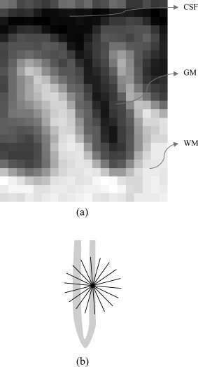
(a) A sulcus in which two sides of the gray matter layer are close to each other. (b) How the algorithm might overestimate the thickness if no stopping criteria were used.

We use the first criterion, since if the probability has been low for a while, we are most likely not in the GM region anymore, and by further summing we would just increase the error. An additional advantage of using this stopping criterion is that summation will be stopped quickly after starting to measure the thickness based on voxels that are not in the GM region. The algorithm will ignore those points and will return near‐zero values for the GM thickness at those locations.

The second condition happens when two parts of the GM layer are so close to each other that the probability on the gap between them is not small enough for the first stopping condition to become true, therefore the algorithm stops summing after identifying a valley on the probability map. As we see in the Appendix, the algorithm can be implemented such that gaps as narrow as one voxel are detected by the above stopping criteria.6

RESULTS AND DISCUSSION

Artificial Data

To illustrate and validate our approach, we first show results using artificial input data.7 Figure 5a, shows the isosurfaces of an artificially created probability map of a parabolic‐shaped layer of GM with varying thickness in a volume of 50 × 50 × 50 voxels. The two isosurfaces represent the inner and outer gray matter surfaces. Depicted as small circles, a number of sample points have been selected, where the computed thicknesses are illustrated as line segments. The direction of each line segment is the optimal direction that gives the minimum line integral of the probability map. The thickness is indicated in the figure by the length of the line segments. To demonstrate the sensitivity and robustness of our algorithm to noise, we added zero‐mean Gaussian noise to the probability map, each time with a different standard deviation. We then computed the mean relative error in the thickness, depicted in Figure 5b, using the thickness obtained in the noiseless case as the ground truth. As expected from an approach based on integration, a linear behavior is encountered. Of course the standard deviation of the relative error in the computed (noisy) thickness behaves like the standard deviation of the noise scaled by the inverse of the square root of the segment length, meaning that by increasing the resolution, this error is decreasing and the noise in the computation is reduced.

Figure 5.

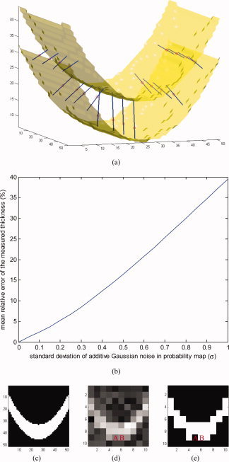
Results on an artificial probability map. (a) Inner and outer surfaces of a parabolic‐shaped layer of “GM” are depicted. Line segments are chosen by the algorithm such that they give the smallest integrals (of the probability map) among all line segments passing through every selected test point, here shown as small circles. (b) Relative error in measured thickness, introduced by additive Gaussian noise. (c) A 2D slice of the volume. (d) The same slice in a five‐times‐lower‐resolution volume with additive Gaussian noise. (e) Binary classification of the low‐resolution volume. [Color figure can be viewed in the online issue, which is available at www.interscience.wiley.com.]

Next, to show the negative consequences of hard segmentation when noise and partial volume effects are present, we reduced the resolution of the volume five times by taking the mean value of every 5 × 5 × 5 subvolume; we also added zero‐mean Gaussian noise with standard deviation of 0.2 (Fig. 5d), and ran our measurement algorithm on it. In addition, we performed hard segmentation on the low‐resolution, noisy volume, by substituting the probability values less than 0.5 with 0 and other values with 1 (Fig. 5e), and re‐ran the measurement algorithm. Using the results of the original high‐resolution case as ground truth, the experiments on the low resolution and noisy volumes showed an average error in the estimated thickness of 1.9 voxels in the segmentation‐free case and 2.2 voxels when hard segmentation was performed as a prestep for reporting this measurement.

As a further demonstration of the robustness to noise of our soft‐classification based algorithm, consider voxels A and B in Figure 5d. As implied by the symmetry of the original object, the two voxels had equal values (of about 0.5) before the noise was added, which changed the values of A and B to about 0.4 and 0.6, respectively. Since the contributions of these two voxels to line integrals differ from the original value only by a small amount of 0.1, our algorithm results in fairly accurate local thicknesses around A and B. On the contrary, the hard classification wrongly categorizes the two (noisy) voxels differently, as “outside” and “inside” (Fig. 5e) which affects the measured local thickness noticeably, resulting in significantly different thickness values around A and B.

Real MRI Data

We tested the proposed technique on 44 T1‐weighted brain MRI scans, acquired using a standard sagittal 3D MP‐RAGE sequence (TR: 2400 ms, minimum TE, inversion time (TI) 1,000 ms, flip angle: 8°, 24 cm field of view), with a reconstructed voxel size of 0.9375 × 0.9375 × 1.2 mm³. To adjust for scanner‐ and session‐specific calibration errors, standard corrections were made for gradient nonlinearity, phantom‐based scaling, and adjustment of intensity inhomogeneity [Leow et al.,2005]. The actual tissue probabilities needed in our method are computed following the procedure explained in the Appendix. All computations are done in native space.

A 2D slice from an MRI volume is shown in Figure 6a along with its computed thickness map in Figure 6b. Since we do not extract the GM, the results also contain thickness values for other parts of the head such as the scalp, which may be ignored. As shown in the figure, at this stage the algorithm cannot detect some sulci/gyri where the resolution is too low and two parts of the outer surface touch each other. However, the technique developed by Teo et al. [1997], can be used in this case to split the merged gray matter, and then compute the corresponding tissue thickness for each part. Figure 6c illustrates a 3D surface‐based mapping of the cortical thickness visualized by the mrGray software, using the steps in [Teo et al.,1997]. As can be seen, although the computed thickness values are volumetric data, it is trivial to map them back onto the mesh (as mrGray was used here to do so), to make them usable by other mesh based software. We also note that smoothing data across the cortex—an essential step for voxel/vertex wise statistics—may also be done before performing a group statistical analysis of cortical thickness. One approach to do this is by Laplace‐Beltrami smoothing of the scalar field on a mesh by using a covariant PDE [Chung et al.,2001; Lerch et al.,2005], or by Laplace‐Beltrami smoothing using an implicit function whose zero level set is the cortical surface [Memoli et al.,2004].

Figure 6.

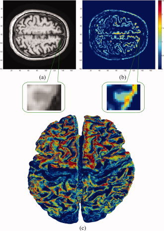
Experimental results on MRI data. All computations were done in 3D. A zoomed‐in version of a sulcus is shown where low resolution results in overestimation of the cortical thickness. (a) A slice of the original volume. (b) The thickness map of the same slice (blue thinner, red thicker). (c) 3D mapping of the cortical thickness. Note the thinner areas in the pre/post central gyri. [Color figure can be viewed in the online issue, which is available at www.interscience.wiley.com.]

Our dataset includes pairs of scans over a 1‐year interval from 22 subjects (total of 44 scans), of whom nine had been diagnosed with Alzheimer's disease at their first scan, and 13 were age‐matched normal subjects. These subjects were included in one of our prior morphometric studies, where the scanning protocol is detailed [Hua et al.,2008]. Each subject was scanned at 1.5 Tesla with a 3D T1‐weighted acquisition, with the following parameters: repetition time (TR), 2,400 ms; minimum full TE; inversion time (TI), 1,000 ms; flip angle, 8°, 24 cm field of view, yielding a reconstructed voxel size of 0.9375 × 0.9375 × 1.2 mm³. The images were calibrated with phantom‐based geometric corrections to ensure stable spatial calibration over time [Jack et al.,2008].

For comparison,8 we also analyzed our data using the FreeSurfer thickness computation technique, [Fischl and Dale,2000]. The results of the change in the mean thickness over a year are demonstrated for the individual cases in Figure 7, while the corresponding detailed statistical data can be seen in Table I. From the computational point of view, our approach is 1–2 orders of magnitude faster than the one implemented in FreeSurfer, and it is highly parallelizable (note of course that FreeSurfer computes other characteristics as well, while we concentrate here on the tissue thickness computation step).

Figure 7.

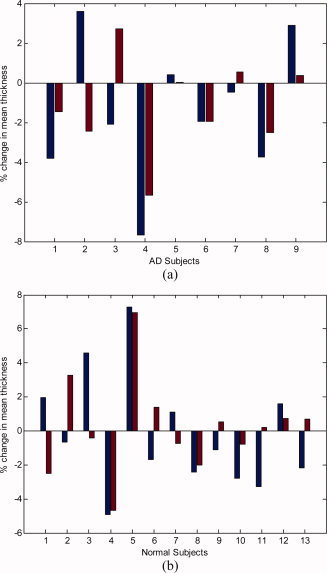
Relative change in the mean cortical thickness over a 1‐year interval, comparing our results (left blue bars) with the results from FreeSurfer (right red bars). (a) Subjects diagnosed with Alzheimer's disease (AD). (b) Normal elderly subjects. [Color figure can be viewed in the online issue, which is available at www.interscience.wiley.com.]

Table I.

Statistical results on real MRI data

Quantity	Proposed algorithm	FreeSurfer
Mean change for all subjects	−0.69%	−0.35%
Mean change for AD subjects	−1.42%	−1.15%
Mean change for normal subjects	−0.19%	+0.20%
SD of change for all subjects	3.42	2.68
SD of change for AD subjects	3.52	2.40
SD of change for normal subjects	3.39	2.82
Group separation	0.36	0.50

The relative change in the mean thickness as measured over a 1‐year interval.

Group separation = (Mean for normal − Mean for AD)/(SD for all).

Both techniques are able to detect a systematic change in cortical thickness over time, both in the AD (Alzheimer's disease) group and in controls. Our method found thickness declined in AD (t _paired = −1.200; P = 0.001), and in controls (t _paired = −0.274; P = 0.009); FreeSurfer found thickness declined in AD (t _paired = −1.495; P = 0.001), and increased in controls (t _paired = +0.175; P = 0.001).9

First of all, the thickness measures are extremely highly correlated between baseline and follow‐up scan, for both measurement methods and both subject groups. Our technique gives measures that correlated highly over the 1 year time‐interval in AD (P = 0.001) and in controls (P = 0.009), and so did FreeSurfer (P = 0.001 both for AD and for normal subjects).

Second, although changes over time are more difficult to measure than absolute values of thickness, our technique correlates highly with FreeSurfer in the changes it measures (Pearson's r = 0.572; P = 0.0028). This agreement between methods was also found in the group of healthy controls, where changes are minimal (r = 0.583; P = 0.0011), and in the group of AD patients (r = 0.558; P = 0.0047).

The changes over time that were detected by FreeSurfer tended to be a little lower in general than those detected by our method, and satisfied the following least‐squares regression model: Δthickness_FS ∼[0.45 × Δthickness_OurMethod] − 0.04.10 Even so, a Student's t test designed to compare thickness values across the two methods did not recover any systematic biases between methods (t _paired = 0.557, P > 0.05). Our method gives a slightly higher SD in the thickness measures at each time point, and this, together with the fact that these errors may be uncorrelated over time, may also lead to a slightly higher estimation of change. Even so, if the sources of errors/deviations are uncorrelated across subjects, there should be no bias incurred by using one method versus the other.

A number of observations can be made from these experiments and the comparison with FreeSurfer. While the actual exact value of cortical thickness decline is not known for the AD subjects, for biological reasons a net increase is not expected for either of the two populations. This is partly because cortical thinning is a natural process that occurs due to neuronal shrinkage in normal aging, and is accelerated in AD due to cell death and neuronal loss in the cortex. Thereby, any apparent increase points to the difficulty and measurement errors in cortical thickness methods. Both our method and FreeSurfer report a few subjects that show increases (less pronounced with our approach), while on average our proposed method shows decline for both populations (much more significant for the AD subjects, as expected). Even so, FreeSurfer shows a net increase for the control subjects, not very large but still statistically significant. A number of reasons might explain this, including registration issues and segmentation errors, which are minimized in our proposed technique. More advanced soft classification techniques will improve the probability assignments and as a result the accuracy of the thickness computed by the proposed approach. Because of the existence of such intrinsic difficulties in measuring cortical thickness, the simultaneous running of different algorithms, with an evaluation of any inconsistencies or consensus, is an important alternative.

Correlation with Clinical Data

In addition to classification accuracy, it is desirable that any measure of cortical thickness can be shown to be associated with clinical measures of deteriorating brain function. This is because image‐derived measures often serve as a proxy for measures of disease burden that are based on repeated cognitive tests, or pathological tests (lumbar puncture). When we modeled factors that affected rates of thinning in AD, our method found a significant sex difference in the rate of thinning (r = 0.428; P < 0.037), whereas FreeSurfer detected this sex difference at a trend level (r = 0.389; P < 0.060), with women experiencing a more rapid rate of loss. Overall, the correlations with clinical measures in AD, such as the Mini‐Mental State Exam scores at baseline and 6 month follow‐up, and the changes in those scores, were around r = 0.37–0.5 for FreeSurfer (P = 0.013–0.073), and slightly lower for our method (r = 0.24–0.30; P > 0.1). Even so, this may be due to the slightly higher standard deviation for the changes reported by our method. Conversely, our method detected associations between the cortical thinning rate and Geriatric Depression Scores (r = 0.433; P = 0.0215), but FreeSurfer did not detect such an association (r = 0.106; P > 0.1). Clearly, a head‐to‐head comparison on a larger sample would be useful, including, for example, assessments of the sample sizes needed by both approaches to detect a 25% slowing of the disease with 80–90% power.

CONCLUSION

We presented a new definition of cortical thickness along with an algorithm for computing it. We were motivated by the importance of measuring the thickness of the cerebral cortex for quantifying the progression of various neurodegenerative brain diseases. Our method calculates the thickness at each voxel, by computing all line integrals of the probability map of the gray matter passing through that voxel, and choosing the minimum integral value. Two stopping criteria are taken into consideration to address issues created by narrow sulci. Unlike most prior work, we take into account the probability of each voxel belonging to the gray matter layer and do not carry out a hard segmentation before measuring the thickness. The proposed algorithm is significantly faster than popular ones such as the one implemented in FreeSurfer. After such accurate voxel‐based computations, the thickness measurements can be mapped into mesh representations if those are needed for other processing steps. This can be done in a number of different ways, e.g., by assigning to each vertex in the mesh the value of the corresponding voxel or a weighted average of nearby voxels. Thereby, the proposed mesh‐free tissue thickness computation can easily be integrated into mesh‐based pipelines, enjoying the best of both representations.

We have validated the technique with artificial data and presented reasonable results for longitudinal MRI scans of Alzheimer's disease and normal subjects. Further improvements are expected when considering, for example, more sophisticated soft‐classification techniques as input to the proposed framework.

We are currently investigating the incorporation of smoothness constraints, where the minimum line integral at a given voxel is influenced by those of neighborhood voxels. This can be done, in principle, by making the optimization a global one, acting on all voxels of interest at once, and adding a penalization term for large local deviations of the corresponding minimal line. The main challenge here to be addressed is the computational one. Note of course that smoothness can also be incorporated as part of the pre‐processing probability computation and/or as part of a post‐processing step after the tissue thickness and minimal lines have been computed. We are also applying the framework introduced here to large population studies.

We now explain in detail how we implemented our proposed algorithm. The input to the algorithm is the raw MRI dataset which is in the form of a three‐dimensional matrix, and the result is the thickness map volume with the same size and spatial sampling as the input.

Computing the Probability Map

We consider the probability of each voxel belonging to the GM as a Gaussian distribution on the intensity value of the voxel in the MRI volume. The mean of the Gaussian is the mean value of manually‐selected sample voxels in the GM, while the standard deviation is the difference between the manually estimated mean values of GM and WM. We could use more sophisticated soft classification algorithms, such as Partial‐Volume Bayesian algorithm (PVB) [Laidlaw et al.,1998], Probabilistic Partial Volume Classifier (PPVC) [Choi et al.,1989], and Mixel classifier [Choi et al.,1991], to further improve the results. Before segmentation, several pre‐processing steps were applied to ensure the accurate calibration of the scans over time and across subjects. Specifically: (1) a procedure termed GradWarp was applied for correction of geometric distortion due to gradient nonlinearity [Jovicich et al.,2006], (2) a “B1‐correction” was applied, to adjust for image intensity non‐uniformity using B1 calibration scans [Jack et al.,2008], (3) “N3” bias field correction, for reducing intensity inhomogeneity caused by non‐uniformities in the radio frequency (RF) receiver coils [Sled et al.,1998], and (4) geometrical scaling, according to a phantom scan acquired for each subject [Jack et al.,2008], to adjust for scanner‐ and session‐specific calibration errors. In addition to the original uncorrected image files, images with all of these corrections already applied (GradWarp, B1, phantom scaling, and N3) are available to the general scientific community (http://www.loni.ucla.edu/ADNI).

Preparing the Masks

To compute the line integrals, we made separate cubic mask volumes for all the line segments, which are in different quantized directions in three‐dimensional space. The length of each dimension of the mask volumes was chosen to be slightly longer than the actual length of the line segment. However, since binary masks are highly inaccurate to apply in numerical integration, we considered continuous mask volumes. We first built binary masks four times bigger in each dimension, and instead of line segments, we considered cylinders four times longer than the line segments with diameter four. Next, we applied a low‐pass filter to it and downsampled the results to achieve the desired non‐binary masks (note that this smoothing acts on the mask, not on the actual MRI data). They were afterwards normalized so that the values in each mask added to the length of the line segment. A two‐dimensional example is depicted in Figure A1.

Figure A1.

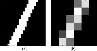
Illustration of how line integral masks are generated. (a) A high‐resolution binary mask, which is four times larger in each direction, is first generated. (b) The real‐size nonbinary mask is produced by downsampling the binary mask.

The directions were chosen by quantizing the unit hemisphere uniformly, as the complete sphere would have been redundant. In the standard spherical coordinates, the unit hemisphere was sampled every 10° in the latitudinal direction, whereas the longitudinal sampling rate varied as follows:

This particular quantization was chosen in order to achieve a relatively constant surface sampling rate, since the solid angle would be

In addition, each mask contained only half of its corresponding line segment (extending from the origin to one point on the hemisphere), given that the two halves were identical and also that the line integrals on them would later need to be taken separately.

Next, the mask volumes were stored in a sparse format that is a list of nonzero elements with their coordinates. To facilitate the integration, elements were sorted into ascending order with respect to their Euclidean distance from the origin. The masks were then stored for further use in the numerical integration step, for various input data.

Numerical Integration

We now briefly explain how the line integrals of a probability map are numerically calculated. To compute the thickness measure at each given voxel, we integrate the probability map on line segments centered at that voxel in different directions using the precomputed mask volumes, and then choose the smallest integral value as the local thickness. Since our stopping criteria make the entire operation nonlinear, we are not able to use convolution methods—which are computationally faster if done in frequency domain, although demanding more memory—to compute the line integrals.

Each line integral is computed in two similar phases. Starting from the main voxel for which we intend to compute the thickness, in each phase we advance in one of the two opposite directions, using the mask volume in the first phase, and its symmetry about the origin (with negated coordinates) in the second phase. In each phase, we start adding the probability values on the region around the main voxel using as weights the values in the sparse form of the corresponding mask. Since the nonzero elements of the mask are sorted into ascending order with respect to their Euclidean distance to the origin, the values of the closer voxels to the main voxel are added first.

The line integral does not need to be entirely computed, since we have a record of the minimum integral value that has been computed so far for a voxel, and we do not need to exceed that. Therefore, the summation continues until one of the following occurs:

• 1All the nonzero elements of the mask are used.
• 2The sum reaches or exceeds the minimum integral value that has so far been computed for that voxel.
• 3One of the stopping criteria becomes true (see the “Algorithm” section).

For the first stopping condition (explained in the “Algorithm” section), a counter is set for the number of successive voxels (with the original sampling size) encountered with probabilities less than the threshold. In this work we used the threshold of 0.3, and summing stopped as the counter reached 10. For the second condition, two states are necessary. In the initial state, a variable counts the number of consecutive decreases in the probability. When it reaches a specific number, the state changes. In the second state, a new variable counts the number of increases in the probability and the summation stops when it reaches a predefined number. In this work 10 was used for both mentioned numbers. Since the masks are made in an interpolative way, they each have many more nonzero voxels than the real length (in voxels) of their corresponding line segments. Therefore, the number of counted iterations is usually about 10 times larger than the actual proceeded length, which results in higher precision in counting. For example, a one‐voxel thick valley can be detected after about five consecutive decreases and five consecutive increases of the probability.

The process of measuring and comparing the thickness for a pair of scans took about 2 to 3 h for our technique, in contrast to 2 to 3 days running time of FreeSurfer (note once again that FreeSurfer is computing a number of different quantities during this time, not limited to tissue thickness). In both cases, a Linux machine with a 2.33 GHz Intel CPU was used. One can also parallelize the above procedure, since it is done independently for each voxel in the volume. For instance, we often divided the volume into eight subvolumes and ran eight parallel jobs in different processors to obtain the thickness map in considerably less time.

Finding the Skeleton

Since the output of the proposed algorithm is the set of thickness values for all the voxels in the volume, we need to find the particular voxels that lie inside the GM layer to compute statistical results for group comparisons.11 A simple GM mask may not necessarily represent the most appropriate set of voxels to examine. Not only might the thickness be underestimated at the voxels close to the inner/outer surfaces, but the values would also be weighted depending on how thick each segment is, i.e., more voxels with the same thickness value are counted on the thicker parts of the GM. Thus, it is best to make a skeleton of the GM, which is a mask with constant thickness positioned in the middle of the layer, far from the inner/outer surfaces. This is of course just one possible way of reporting the rich amount of information produced by the proposed algorithm, where every voxel contains a tissue thickness measurement. The particular way of exploiting this information might depend on the task at hand.

To find the skeleton without explicit segmentation, we modified the algorithm such that for each voxel v, in addition to the total thickness T(v), it reports the two different thickness values t ₁(v) and t ₂(v), the lengths of the two subsegments on each side of the voxel on the optimal line segment (t(v) = t ₁(v) + t ₂(v), see Figure A2). Next, we considered the skeleton to be the set of the voxels with the following properties:

where P(v) is the probability of v belonging to the GM. The first condition guarantees that the skeleton is always at most half a voxel thick, and the two conditions together guarantee that the skeleton remains in the middle of the GM layer.

Figure A2.

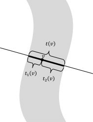
The lengths, t ₁(v) and t ₂(v), of the two sub‐segments are used in finding the gray matter skeleton for computing the cortical thickness variation.

In addition, to better remove the skull and non‐GM parts of the brain, we applied a rough GM mask obtained from FreeSurfer (FreeSurfer was only used for this task).

REFERENCES

- Aganj I,Sapiro G,Parikshak N,Madsen SK,Thompson P ( 2008): Segmentation‐free measurement of cortical thickness from MRI. Proc ISBI 2008: 1625–1628. [DOI] [PMC free article] [PubMed] [Google Scholar]
- Choi HS,Haynor DR,Kim YM ( 1989): Multivariate tissue classification of MRI images for 3‐D volume reconstruction—A statistical approach. Proc SPIE Med Imaging III: Image Process 1092: 183–193. [Google Scholar]
- Choi HS,Haynor DR,Kim YM ( 1991): Partial volume tissue classification of multichannel magnetic resonance images—A mixel model. IEEE Trans Med Imaging 10: 395–407. [DOI] [PubMed] [Google Scholar]
- Chung MK,Worsley KJ,Taylor J,Ramsay JO,Robbins S,Evans AC ( 2001): Diffusion smoothing on the cortical surface. Neuroimage 13 ( Suppl 1): 95. [Google Scholar]
- Fischl B,Dale AM ( 2000): Measuring the thickness of the human cerebral cortex from magnetic resonance images. Proc Natl Acad Sci USA 97: 11050–11055. [DOI] [PMC free article] [PubMed] [Google Scholar]
- Haidar H,Soul JS ( 2006): Measurement of cortical thickness in 3D brain MRI data: Validation of the Laplacian method. Neuroimage 16: 146–153. [DOI] [PubMed] [Google Scholar]
- Hua X,Leow AD,Lee S,Klunder AD,Toga AW,Lepore N,Chou YY,Brun C,Chiang MC,Barysheva M,Jack CR Jr,Bernstein MA,Britson PJ,Ward CP,Whitwell JL,Borowski B,Fleisher AS,Fox NC,Boyes RG,Barnes J,Harvey D,Kornak J,Schuff N,Boreta L,Alexander GE,Weiner MW,Thompson PM ( 2008): 3D characterization of brain atrophy in Alzheimer's disease and mild cognitive impairment using tensor‐based morphometry. Neuroimage 41: 19–34. [DOI] [PMC free article] [PubMed] [Google Scholar]
- Jack CR Jr,Bernstein MA,Fox NC,Thompson P,Alexander G,Harvey D,Borowski B,Britson PJ,L Whitwell J,Ward C,Dale AM,Felmlee JP,Gunter JL,Hill DL,Killiany R,Schuff N,Fox‐Bosetti S,Lin C,Studholme C,DeCarli CS,Krueger G,Ward HA,Metzger GJ,Scott KT,Mallozzi R,Blezek D,Levy J,Debbins JP,Fleisher AS,Albert M,Green R,Bartzokis G,Glover G,Mugler J,Weiner MW ( 2008): The Alzheimer's disease neuroimaging initiative (ADNI): MRI methods. J Magn Reson Imaging 27: 685–691. [DOI] [PMC free article] [PubMed] [Google Scholar]
- Jones SE,Buchbinder BR,Aharon I ( 2000): Three‐dimensional mapping of cortical thickness using Laplace's equation. Hum Brain Mapp 11: 12–32. [DOI] [PMC free article] [PubMed] [Google Scholar]
- Jovicich J,Czanner S,Greve D,Haley E,van der Kouwe A,Gollub R,Kennedy D,Schmitt F,Brown G,Macfall J,Fischl B,Dale A ( 2006): Reliability in multi‐site structural MRI studies: Effects of gradient non‐linearity correction on phantom and human data. Neuroimage 30: 436–443. [DOI] [PubMed] [Google Scholar]
- Kabani N,Le GG,MacDonald D,Evans AC ( 2001): Measurement of cortical thickness using an automated 3‐D algorithm: A validation study. Neuroimage 13: 375–380. [DOI] [PubMed] [Google Scholar]
- Laidlaw DH,Fleischer KW,Barr AH ( 1998): Partial‐volume Bayesian classification of material mixtures in MR volume data using voxel histograms. IEEE Trans Med Imaging 17: 74–86. [DOI] [PubMed] [Google Scholar]
- Leow AD,Klunder AD,Jack CR,Toga AW,Dale AM,Bernstein MA,Britson PJ,Gunter JL,Ward CP,Whitwell JL,Borowski B,Fleisher A,Fox NC,Harvey D,Kornak J,Schuff N,Studholme C,Alexander GE,Weiner MW,Thompson PM ( 2005): Longitudinal stability of MRI for mapping brain change using tensor‐based morphometry. Neuroimage 31: 627–640. [DOI] [PMC free article] [PubMed] [Google Scholar]
- Lerch JP,Evans AC ( 2005): Cortical thickness analysis examined through power analysis and a population simulation. Neuroimage 24: 163–173. [DOI] [PubMed] [Google Scholar]
- Lerch JP,Pruessner JC,Zijdenbos A,Hampel H,Teipel SJ,Evans AC ( 2005): Focal decline of cortical thickness in Alzheimer's disease identified by computational neuroanatomy. Cereb Cortex 15: 995–1001. [DOI] [PubMed] [Google Scholar]
- Lohmann G,Preul C,Hund‐Georgiadis M ( 2003): Morphology‐based cortical thickness estimation. Inf Process Med Imaging 18: 89–100. [DOI] [PubMed] [Google Scholar]
- MacDonald D,Kabani N,Avis D,Evans AC ( 2000): Automated 3‐D extraction of inner and outer surfaces of cerebral cortex from MRI. Neuroimage 12: 340–356. [DOI] [PubMed] [Google Scholar]
- Mémoli F,Sapiro G,Thompson PM ( 2004): Implicit brain imaging. Neuroimage 23 ( Suppl 1): S179–S188. [DOI] [PubMed] [Google Scholar]
- Miller MI,Massie AB,Ratnanather JT,Botteron KN,Csernansky JG ( 2000): Bayesian construction of geometrically based cortical thickness metrics. Neuroimage 12: 676–687. [DOI] [PubMed] [Google Scholar]
- Pham DL,Bazin PL ( 2004): Simultaneous boundary and partial volume estimation in medical images. Proc MICCAI 2004, 119–126. [Google Scholar]
- Pizer S,Eberly D,Fritsch D,Morse B ( 1998): Zoom‐invariant vision of figural shape: The mathematics of cores. Comput Vis Image Understanding 69: 55–71. [Google Scholar]
- Scott MLJ,Thacker NA ( 2004): Cerebral cortical thickness measurements. Tina Memo 2004–2007, Manchester, England. [Google Scholar]
- Sled JG,Zijdenbos AP,Evans AC ( 1998): A nonparametric method for automatic correction of intensity nonuniformity in MRI data. IEEE Trans Med Imaging 17: 87–97. [DOI] [PubMed] [Google Scholar]
- Teo PC,Sapiro G,Wandell BA ( 1997): Creating connected representations of cortical gray matter for functional MRI visualization. IEEE Trans Med Imaging 16: 852–863. [DOI] [PubMed] [Google Scholar]
- Thompson PM,Hayashi KM,Sowell ER,Gogtay N,Giedd JN,Rapoport JL,de Zubicaray GI,Janke AL,Rose SE,Semple J,Doddrell DM,Wang Y,van Erp TGM,Cannon TD,Toga AW ( 2004): Mapping cortical change in Alzheimer's disease, brain development, and schizophrenia. Neuroimage 23 ( Suppl 1): S2–S18. [DOI] [PubMed] [Google Scholar]
- Thompson PM,Lee AD,Dutton RA,Geaga JA,Hayashi KM,Eckert MA,Bellugi U,Galaburda AM,Korenberg JR,Mills DL,Toga AW,Reiss AL ( 2005): Abnormal cortical complexity and thickness profiles mapped in Williams syndrome. J Neurosci 25: 4146–4158. [DOI] [PMC free article] [PubMed] [Google Scholar]
- Yezzi AJ,Prince JL ( 2003): An Eulerian PDE approach for computing tissue thickness. IEEE Trans Med Imaging 22: 1332–1339. [DOI] [PubMed] [Google Scholar]
- Young K,Schuff N ( 2008): Measuring structural complexity in brain images. Neuroimage 39: 1721–1730. [DOI] [PMC free article] [PubMed] [Google Scholar]