

Abstract
Accurate system modeling in tomographic image reconstruction has been shown to reduce the spatial variance of resolution and improve quantitative accuracy. System modeling can be improved through analytic calculations, Monte Carlo simulations, and physical measurements. The purpose of this work is to improve clinical fully-3-D reconstruction without substantially increasing computation time. We present a practical method for measuring the detector blurring component of a whole-body positron emission tomography (PET) system to form an approximate system model for use with fully-3-D reconstruction. We employ Monte Carlo simulations to show that a non-collimated point source is acceptable for modeling the radial blurring present in a PET tomograph and we justify the use of a Na22 point source for collecting these measurements. We measure the system response on a whole-body scanner, simplify it to a 2-D function, and incorporate a parameterized version of this response into a modified fully-3-D OSEM algorithm. Empirical testing of the signal versus noise benefits reveal roughly a 15% improvement in spatial resolution and 10% improvement in contrast at matched image noise levels. Convergence analysis demonstrates improved resolution and contrast versus noise properties can be achieved with the proposed method with similar computation time as the conventional approach. Comparison of the measured spatially variant and invariant reconstruction revealed similar performance with conventional image metrics. Edge artifacts, which are a common artifact of resolution-modeled reconstruction methods, were less apparent in the spatially variant method than in the invariant method. With the proposed and other resolution-modeled reconstruction methods, edge artifacts need to be studied in more detail to determine the optimal tradeoff of resolution/contrast enhancement and edge fidelity.
Index Terms: Fully 3-D reconstruction, point spread function, positron emission tomography (PET), system modeling
I. Introduction
The goal of this work is to improve the quantitative accuracy of whole-body positron emission tomography (PET) imaging through the use of a more accurate system model, while keeping additional reconstruction computation time to a minimum. We present a practical method for measuring the detector blurring component of the system response with a non-collimated point source. We demonstrate with Monte Carlo simulations that a non-collimated point source can model the radial blurring present in a PET tomograph. Also, we justify the use of a Na22 point source for collecting system response measurements. We measure the system response of a clinical PET system and incorporate this into a modified OSEM method.
Previous efforts have modeled the system response through analytical derivations [1], [2], Monte Carlo simulations [3], [4], and empirical measurements [5], [6] leading to improved resolution and quantitation. Past empirically measured system response functions used line sources positioned at multiple radial locations in the imaging field-of-view (FOV) [5], [7] or time-consuming measurement of point sources positioned at finely sampled locations throughout the imaging FOV [6]. These efforts performed resolution modeling in the system’s projection space. In contrast, several efforts have proposed reconstruction methods with resolution modeled in the reconstructed image space [8]-[10]. In this work, we empirically measure the system response and leave the resolution model in the original measurement projection space. In our implementation, we enforce the resolution model with 1-D convolutions in the reconstruction. In theory, the model could be represented in the image space, but this would require 2-D or 3-D convolutions during reconstruction updates.
Our previous work used Monte Carlo simulations of the system response and evaluated the potential improvements with a simulated system model [11]. In that work, we used simulations to evaluate the incremental benefit with improved modeling of system 1) radial blurring and 2) radial and axial blurring. We showed that the addition of improved radial blurring could improve resolution, quantification, and contrast to noise. The further addition of an axial blurring component lead to only minor gains over the radial only model. These results acknowledge that, for clinical PET system geometries, in-plane parallax error is the most spatially-variant resolution component. This parallax error is primarily a radially blurring component, suggesting that we can recover most of the system resolution losses with a simple radially blurring system model. This prior simulation work motivates our current efforts to physically measure the radial system response and assess the added value of including this response in the reconstruction.
Another argument for limiting the response function to in-plane transaxial radial blur and not cross-plane axial blur is based on the dimensions of the clinical system of interest. The GE Discovery STE (GE DSTE) [12] has a transaxial crystal spacing of 4.8 mm and an axial spacing of 6.4 mm. The larger axial spacing suggests less intercrystal penetration axially and less blur amongst axial bins. Furthermore, the axial oblique angle of incidence with the detector surface is at most 15° at the edge of the transaxial FOV for the most extreme oblique plane. On the other hand, the most extreme in-plane, transaxial angle of incidence is 51°, which confirms that parallax error is primarily in-plane.
The system model for a PET tomograph can be factorized into multiple components such as the geometric projection matrix (basis for all conventional models), attenuation correction factors, detector sensitivity factors, and detector blurring [13]. The complete system model of a fully 3-D imaging system is a seven dimensional function, with three dimensions to define each object space location which contributes to each data space location defined with four dimensions. This work simplifies the model of the detector blurring and other resolution degradations, as a 2-D system response function, S(s; sv), that blurs in radial position, s, and is variant in radial position sv. This term includes effects due to inter-crystal scatter, penetration, and, since it is a measured response, photon pair noncollinearity and positron range. Because this term includes more than just detector effects, we use the more general term “point spread function,” as opposed to “detector blurring [7],” to describe a model with all of these effects. We assume rotational invariance of the detector geometry and invariance amongst axial planes; thus, the same response function can be applied at all azimuthal angles and axial planes.
This work extends our previous preliminary studies [14], [15] to include the measurement of the system model on a modern whole-body PET tomograph and the thorough evaluation of resolution, contrast and noise with measured phantom and patient data. Specifically, here we 1) justify the measurement of the system model with non-collimated Na22 point sources positioned at limited locations in the FOV, 2) empirically measure the point spread function (PSF), 3) apply the PSF to a fully-3-D reconstruction method, and 4) evaluate the resolution, contrast, and noise properties with measured phantom and patient data.
II. Development of Spatially Variant System Model
A. Collimated Versus Non-Collimated
We propose using measured, empirical response data from a whole-body PET tomograph to characterize the point spread function of the system. An ideal experiment would employ a point source collimated to emit photons along a single line of response (LOR), revealing the blurring extent in each LOR. In reality, this experiment is not feasible because of: 1) the number of LORs, 2) the challenge of accurately positioning the point source and the collimation given the multiple degrees-of-freedom, and 3) an appropriately collimated source results in significantly fewer photons requiring long scan times for each LOR.
The use of a non-collimated point source avoids these challenges; but, for 2-D imaging, data from a non-collimated point source does not contain information about blurring among azimuthal angles considering that all angles are collected during acquisition. In order to justify the use of the non-collimated measured point source, we performed Monte Carlo simulations using the GATE package [16] to show that collimated and non-collimated point sources result in similar S(s; sv) response functions. We simulated a dual photon emitting source in a validated scanner model of the General Electric (GE) Advance PET scanner [17]. These simulations include the effects of scanner geometry, block effects, inter-crystal scatter, and penetration and were postcorrected to have equally spaced radial bins as performed on the Advance system. The Advance scanner has a radial bin spacing of 1.97 mm at the center of a 550 mm transaxial FOV.
For each simulated data set of an acquisition of a point source at radial location sv, we draw profiles through the radial bins s for a fixed azimuthal angle. Fig. 1 plots the radial full-width at half-maximum (FWHM) and FWTM of the resulting S(s; sv) from the point sources positioned at different radial positions. These plots show results from 10 different simulations (collimated and non-collimated point source at five unique radial positions). The close agreement in these plots, with ~ 1 mm difference in FHWM at all locations, shows that a non-collimated point source is adequate for measuring the system response function S(s; sv). The validity of this conclusion is further confirmed in Fig. 2 where the shape of the simulated noncollimated and collimated responses are shown to be very similar and match the measured response from a Na22 point source in the GE Advance.
Fig. 1.

FWHM and FWTM of S(s; sv) formed from non-collimated and collimated point source at different locations.
Fig. 2.
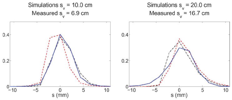
Comparison of S(s; sv) from simulated collimated (dash dot), simulated non-collimated (dash), and measured non-collimated (solid) point sources. The y-axis is normalized units such that each S(s; sv) has anarea under the curve of one.
B. Positron Range of Point Source
A point source of one of the typical PET radioisotopes is difficult to fashion in a reproducible manner and the relatively short half life complicates a longer experiment needed to characterize the system. Consequently, we used a solid Na22 source (half life = 2.6 years) of size ~ 0.25 mm diameter embedded in Lucite.
One concern with using the Na22 source is its potentially different positron range than clinical PET isotopes.We used a modification of the SimSET simulation package [18] to model the positron range of Na22 and F18 [19]. This model is based on the Palmer and Brownell parameterized model [20]. Rather than following the positron trajectory until is reaches thermal energy [21], this model assumes that the equilibrium particle density resulting from a point source of mono-energetic positrons can be represented by a 3-D Gaussian distribution centered at the origin.
We simulated the positron end points of F18 in water (clinical scanned object) and Na22 in Lucite (our method for measuring response). Fig. 3 shows the calculated positron annihilation coordinates in various representations (projection of 3-D positron endpoint cloud projected onto a plane, a single axis, and a histogram of positron distances). These plots reveal that the positron ranges for F18 and our proposed source are very similar and justify the use of Na22 for system response function measurements.
Fig. 3.

Comparison of positron range of F18 in water (a) and Na22 in Lucite (b). Binary images (a) and (b) show positron annihilation coordinates projected on a single axis. Plot (c) shows the projection of (a) and (b) onto a single axis with F18 (solid) and Na (dashed). The histogram (d) reveals of positron distance of F18 (solid) and Na (dashed).
C. Measurement Spacing
Whole-body PET scanners have gaps between detector blocks. In an effort to assess the effect of the block gap on the radial response, we performed measurements of the Na22 point source at multiple locations around these gap transitions. In the GE DSTE scanner, we acquired multiple measurements of the point source at y = 4 mm and x = i × 2.54 mm from the center of the transaxial FOV for i = 0 to 14. We also measured at the edge of the FOV at y = 4 mm and x = −310 + i × 2.54 mm for i = 0 to 13. This scanner contains 560 BGO crystals in each ring with a 4.7 mm tangential crystal spacing. The scanner measures a total of 329 radial bins and a 2.1 mm block gap occurs once every 15 radial bins.
The data were corrected for detector efficiency normalization. Fig. 4 presents profiles through radial bins for azimuthal angle zero for 15 separate acquisitions. Profiles are normalized to have matched areas under the curve. All profiles are presented on the same axis with alternating line type to show that the general shape of the response does not change dramatically even at the block gap locations. Likewise, the profiles from the center of the FOV (Fig. 4) reveal the characteristic symmetric triangular response and the profiles from the edge of the FOV (Fig. 5) are asymmetric due to increased inter-crystal penetration. These profiles suggest that the radial PSF is smoothly varying and that we do not need to measure the effects of block gaps on the radial PSF with this scanner. As a result, we will coarsely sample the PSF.
Fig. 4.

Radial profiles through 15 separate sinogram data sets at azimuthal angle 0 for a point source positioned at 15 locations sv = 2.5 mm through 38.1 mm. Data acquired from point source measurements at center of transaxial FOV. Second row contains profiles shifted to have same max location. These radial bins have an average spacing of 2.5 mm.
Fig. 5.

Radial profiles through 14 separate sinogram data sets at azimuthal angle 0. Data acquired from point source measurements at edge of transaxial FOV for a point source positioned at 14 location sv = −310 mm through −274.4 mm. Second row contains profiles shifted to have same max location. These radial bins have an average spacing of 1.9 mm.
D. Measurement of Point Spread Function
Based on the results above, we measured the PSF with a 5.6 kBq Na22 point source of size ~ 0.25 mm diameter embedded in Lucite. We acquired non-collimated measurements of the Na22 point source positioned at 14 locations from the center to the edge of the transaxial FOV in the GE DSTE PET/CT scanner. The profile through the measured data at a fixed azimuthal angle provided the radial response for a given location.
We assume that the location of the maximum value for each kernel is the location of the point source. In smaller, high-resolution animal systems, mispositioning of the maximum value can be common. For this clinical system, we performed a side study consisting of point sources (at multiple known locations) and found that mispositioning errors with using the max location are at most 1 radial bin at the edge of the transaxial view. For simplicity, we did not include this minor effect in our model.
In order to find the PSF at all radial locations, we parameterized the radial response from 12 of these measurements with their discrete cosine transform (DCT) coefficients. The linear fit of these coefficients provided the DCT at all radial positions in the FOV. The inverse DCT at each position provided interpolated radial blurring kernels. Assuming transaxial symmetry, this function is flipped in s for the other half of the transaxial FOV. We originally proposed this parameterization approach for 3-D system responses derived from simulations [11]. Fig. 6 presents the radial blurring kernels which blur among radial bins s dependent on radial bin location sv.
Fig. 6.

Isocontour plot of radial blurring kernels interpolated to all radial positions, sv.
To provide an independent confirmation of this parameterized model, we compared the model with the two measured responses which did not contribute to the model. Fig. 7 presents independent radial profiles from separate measurements and from the parameterized PSF. The close match provides confidence in the accuracy of the parameterized model. The measured PSF is similar in shape and extent to the 2-D PSF we simulated in previous work [11].
Fig. 7.

Measured radial profiles (solid) and parameterized radial profiles (dashed) at positions 118 mm and 184 mm from center of FOV.
E. Applying PSF in Reconstruction
We started with an accurate fully-3-D reconstruction that models all of the physical effects (attenuation, scatter, randoms, efficiencies, and line-of-response locations with a model of detector sizes) within the loop of the algorithm and will be denoted as OSEM+LOR. This method is derived from efforts of Manjeshwar et al. [22] and reconstructs using angular subsets and all oblique planes from the fully 3-D data (no axial mashing). We modify OSEM+LOR with the PSF modeled as a 2-D function S which blurs across radial bins and is variant in the radial location. The geometric projection matrix, P̃, which analytically calculates the intersection of each detection line-of-response, i, with voxel, j, is modified to form the complete system model P as
| (1) |
for a system with N total measurements. The reconstruction method which incorporates the spatially variant PSF will be denoted as OSEM+LOR+PSF.
The applied S was a blurring kernel with 11 bins in radial s that varied at each radial location sv. This kernel equated to roughly 2–3 cm in length depending on location in FOV. The blurring terms were incorporated in a factorized system model and applied during each call to the system matrix, both in the forward and backprojection operations.
The spatially variant model was compared with an invariant model that used a fixed blurring kernel throughout the FOV. This fixed kernel was formed by averaging the radial blurring kernels from the central 40 cm of the FOV. This averaging was intended to find an invariant kernel which is roughly appropriate for the most common imaging region. The incorporation of the spatially invariant PSF model will be denoted as OSEM+LOR+invPSF.
III. Evaluation Methods
We reconstructed fully-3-D data measured on the GE DSTE PET/CT scanner. For these studies, all corrections were applied to the data inside the iterative loop of OSEM essentially preserving the Poisson statistics of the measurements. We compared: OSEM with a projector operating on equally spaced radial bins (OSEM), OSEM with the accurate line-of-response projector (OSEM+LOR) [22], the spatially invariant PSF reconstruction (OSEM+LOR+invPSF), and the spatially variant PSF reconstruction (OSEM+LOR+PSF).
A. Line Source Phantom
We constructed a custom line source phantom consisting of an elliptical chamber (30 cm long axis, 22 cm short axis, and 18 cm deep). An acrylic frame was suspended in the elliptical chamber to support multiple lengths of tubing (12 cm long, 0.8 mm internal diameter). The tubing formed eight line sources 3.5 cm apart along the long axis of the phantom. The line sources were filled with F18 and either A) imaged in air or B) imaged with a warm uniform activity concentration background with a roughly 200:1 line to background ratio. The phantom was positioned in the upper half of the scanner with the line sources oriented parallel to the scanner axis as shown in Fig. 8. This enabled the evaluation of transaxial resolution at radial locations ranging from the center to the edge of the scanner from a single image volume.
Fig. 8.

Illustration of transaxial view of line source phantom positioned in 70 cm bore of scanner.
For each reconstructed image volume, we draw a radial profile and tangential profile through the line source on the transaxial image. For the profiles through the warm background images, we subtract the baseline background activity. The full-width at half-maximum (FWHM) of the radial and tangential profiles are averaged to provide a measure of average transaxial resolution for each of the eight line sources. The line sources traverse 30 slices in the image volume. We measure resolution on eight neighboring transaxial slices to provide an estimate of the mean and error in the resolution measurements. We measure noise in the warm uniform activity background images as the coefficient of variation (COV) of voxel values in a large volume of interest positioned in the background.
B. NEMA IQ Phantom
Contrast was evaluated with the NEMA IEC body phantom consisting of an anthropomorphic chamber containing six hot spheres with diameters 10, 13, 17, 22, 28, and 37 mm [23]. The phantom was filled with Ge68 to have a 4:1 sphere to background activity ratio. We performed 50 5-min fully 3-D acquisitions to provide 50 independent realizations of data. Each realization contained 85 million counts.
For each sphere in each image volume, we compute the contrast recovery coefficient (CRC) of the mean value of the sphere. This is defined as the difference between the mean value of the sphere and the true value divided by the true value.
We calculate noise by computing the coefficient of variation (COV) of the mean value of a region of interest (ROI) across the 50 realizations. We compute this multirealization COV for 60 ROIs positioned on five slices and average this to estimate the average variability across realizations. This noise is arguably more reflective of the true noise in the background, but is rarely computed in image quality evaluations because there is rarely access to multiple independent realizations.
For a 20 × 20 pixel uniform region on one target-absent slice, we calculate the sample correlation matrix over the 50 realizations. One row in the correlation matrix corresponds to how a particular pixel is correlated with neighboring pixels. We select the row (1 × 400 vector) corresponding to a center pixel in the 20 × 20 region, and arrange it into a 20 × 20 image to visualize a single pixel’s correlation with neighbors. We call this image the local correlation image. Due to the limited number of realizations leading to a noisy sample correlation matrix, we average matrices from three target-absent slices.
C. Whole-Body Patient Exam
We also evaluated a whole-body fully 3-D PET/CT exam from a 109 kg patient, scanned one hour after a 370 MBq injection of F18-fluorodeoxyglucose (FDG). The patient was scanned with 5 min per bed position for a total of six bed positions. The patient was scanned postchemotherapy leading to an increased uptake in bone marrow, which offers the added value of numerous high resolution features for evaluation.
D. Brain Patient Exam
We reconstructed fully 3-D brain data of a 77 kg patient scanned for 15 min, 1 h after a 296 kBq FDG injection.
IV. Evaluation Results
We present results from volumetric reconstructions with 256 × 256 voxels per slice using 28 subsets for each iteration. The addition of our PSF model or invPSF model to OSEM+LOR increased the reconstruction time by 3.2%.
A. Line Source Phantom
Transaxial slices from the line source in warm background were reconstructed from a fully 3-D acquisition with 560 × 106 events and appear in Fig. 9. Visual inspection reveals a different noise structure between OSEM+LOR and OSEM+LOR+PSF and potentially improved resolution with the PSF method. The cold spots at the top and bottom of the phantom are from the frame which supports the line-sources. The FHWM measured from the line source data appear in Fig. 10. When the line sources are measured in air (with a total of 46 × 106 events), the proposed PSF model resulted in 2 mm radial resolution at all locations in the FOV. The invariant PSF resulted in images with slight spatial variance in the resolution. The resolution results are markedly different when the line sources are in a more realistic imaging scenario surrounded by a scattering medium and activity. When measured with a warm background, the radial resolution degraded to 2.5–4 mm and was dependent on radial location. Increasing the number of iterations to 20 did not dramatically improve the resolution with the PSF and the resolution remained spatially variant (albeit not as spatially variant as OSEM+LOR). For all lines, the invariant PSF reconstruction resulted in slightly worse resolution than the variant PSF reconstruction. It is worth noting that the line sources in air resolution values are highly dependent on pixel size; the final resolution can be reduced by simply reducing the reconstructed pixel size.
Fig. 9.

Reconstructions of line source phantom with OSEM+LOR (first row), OSEM+LOR+PSF (second row), and radial profile (third row) after the completion of different iterations (noted in heading). The subheading for each image contains the range and mean value of the image in kBq/cc. The radial profiles extend vertically through the second to most extreme radially positioned line source (22.4 cm from center of FOV) and are presented for OSEM+LOR (+) and OSEM+LOR+PSF (○). Average radial FWHM listed in each profile plot.
Fig. 10.

Average transaxial resolution versus location measured from phantom with eight axial line sources with first column from line sources in air, second column from line sources in warm background after 10 iterations, and third column from line sources in warm background after 20 iterations. Error bars denote the standard error in the estimate of the mean FWHM values across eight neighboring transaxial slices. The solid line is fit to the mean FWHM values to show trend with radial locations. All reconstructions with 28 subsets, no postfilter, 1.37 mm/pixel.
Fig. 11 presents the resolution metric at 5.1 cm and 22.5 cm from the center of transaxial FOV versus image update. Fig. 12 presents FWHM versus the coefficient of variation in the background voxels. The FWHM of the PSF method takes longer to converge to a final value than OSEM and has resolution improvements at matched background noise (with noise defined as voxel to voxel variability).
Fig. 11.

Transaxial resolution at 5.1 cm (left) and 22.2 cm (right) versus image update measured from phantom with 8 axial line sources in warm background.
Fig. 12.

Transaxial resolution at 5.1 cm (left) and 22.2 cm (right) versus coefficient of variation in background voxels from line sources in warm background phantom. Lines parameterized by every iteration with initial images in upper left and 20 iterations, 28 subsets image in lower right.
B. NEMA IQ Phantom
Figs. 13 and 14 present reconstructions of one of the 50 acquisitions of the NEMA phantom and profiles through these images. This acquisition contains the count density of a typical clinical acquisition. Figs. 15 and 16 present the mean and standard deviation image from 50 independent acquisitions of the NEMA phantom, each reconstructed with 28 subsets, eight iterations. At this iteration, the standard deviation images reveal that OSEM+LOR+PSF has less noise than OSEM+LOR; the average of the standard deviation image is 40% lower with OSEM+LOR+PSF. Profiles through the mean and standard deviation images appear in Fig. 17. Showing improved contrast with the use of a PSF model and reduced standard deviation amongst realizations at a matched iteration level.
Fig. 13.

Zoomed transxial view of NEMA IQ phantom from one of 50 acquisitions. Each image reconstructed with different algorithm after eight iterations.
Fig. 14.

Profile through transaxial slice from one of 50 acquisitions of NEMA IQ phantom (profile through slices in Fig. 13). Dashed lines mark true background and hot sphere values.
Fig. 15.

Mean of 50 independent images of NEMA IQ phantom reconstructed with different algorithms after eight iterations. Top row contains transaxial view; bottom row contains coronal view.
Fig. 16.

Standard deviation of 50 independent images reconstructed with different algorithms after eight iterations. OSEM+LOR+PSF has the lowest deviation across realizations. All images have a matched colorscale.
Fig. 17.

Profile through transaxial slice of mean image (top) and standard deviation image (bottom) after eight iterations. Dashed lines mark true background and hot sphere values.
Fig. 18 presents contrast recovery coefficients (CRC) of mean sphere values for images after eight iterations. As with the resolution results, the PSF algorithm requires more iterations to reach a final value. The CRC versus multirealization noise appears in Fig. 19. These plots are parameterized by iteration number. The proposed OSEM+LOR+PSF provides a 8% improvement and the OSEM+LOR+invPSF provides a 10% improvement over OSEM in average CRC of mean sphere values at a matched background noise of 10% variability. A two-sample t-test of CRC from method 1 to method 2 for each sphere size confirmed that the CRC for all four methods are significantly different from each other (each sphere for all method to method tests resulted in p < 0.05).
Fig. 18.

Contrast recovery coefficient (CRC) for mean value of sphere versus sphere size after 8 iterations. Error bars mark the standard deviation of CRC values across the 50 independent acquisitions.
Fig. 19.

CRC versus “true” noise (bottom) for 35 cm background ROI. Error bars denote standard deviation in CRC across 50 realizations. Circles mark end of 4 and 8 iterations.
Fig. 20 presents the local correlation images for a region of the background. The use of PSF in the reconstruction leads to higher positive correlations amongst neighboring pixels (larger positive region in correlation image) as also evident in the noise texture in the reconstructed images.
Fig. 20.

Local correlation images for a pixel in the background of the NEMA IQ phantom. OSEM+LOR (left) and OSEM+LOR+PSF (right) correlation images show correlation of 1 with itself (center of image) and positive and negative correlations with neighboring pixels.
C. Whole-Body Patient Exam
Coronal images from the whole-body PET/CT exam appear in Fig. 21 with 0 mm, 3.5 mm, and 7 mm Gaussian postfilter to represent a range of clinical settings. Visual inspection reveals a different noise texture with the OSEM+LOR+PSF with a trend to being less visually noisy and with more contrast enhancement. Fig. 22 presents profiles through the ribs in the patient after 7 mm postfiltering, which is a common clinical setting. Also, we matched the “noise” (pixel-to-pixel standard deviation in the liver) with postsmoothing leading to a 7 mm postsmoothing on the OSEM and 6 mm postsmoothing with PSF. With matched iterations and matched 7 mm postsmoothing, the OSEM+LOR+PSF leads to a 15% higher rib to background soft tissue uptake ratio. With matched pixel-to-pixel variability, there is a 22% higher rib to background ratio.
Fig. 21.

Coronal view of whole-body FDG exam reconstructed with OSEM+LOR (top row) and OSEM+LOR+PSF (bottom row). Images presented after four iterations, 28 subsets with no postfilter (column 1), 3.5 mm postfilter (column 2), and 7 mm postfilter (column 3).
Fig. 22.

Radial profiles through two left ribs from whole-body patient exam from Fig. 21. Profiles through OSEM+LOR with 7 mm postsmoothing, OSEM+LOR+PSF with 7 mm postsmoothing, and OSEM+LOR+PSF with 6 mm postsmoothing, which has matched liver noise with the OSEM+LOR image.
D. Brain Patient Exam
Views of multiple transaxial and coronal slices appear in Figs. 23 and 24 for reconstructions with four iterations, 28 subsets, and 2 mm voxels. The first row of contains images reconstructed with OSEM+LOR. These images were postsmoothed with a 3 mm Gaussian (row 2) to have matched pixel-to-pixel variability in the central white matter with the OSEM+LOR+PSF images (row 3). The OSEM+LOR+PSF results in images with enhanced contrast apparent in the improved ability to resolve the putamen and other fine structures.
Fig. 23.

Two transaxial slices from OSEM+LOR (row 1), OSEM+LOR+3 mm postfilter (row 2), and OSEM+LOR+PSF (row 3). All images have matched color scales and row 2 and row 3 have matched pixel-to-pixel variability in central white matter.
Fig. 24.

Two coronal slices from OSEM+LOR (row 1), OSEM+LOR+3 mm postfilter (row 2), and OSEM+LOR+PSF (row 3). All images have matched color scales and row 2 and row 3 have matched pixel-to-pixel variability in central white matter.
V. Discussion
Our previous work used simulations to show the benefits of a simulated system model both in terms of resolution and variance across multiple realizations [11]. This current work expanded upon the previous simulation studies and empirically measured the system response function and applied this function to measured, not simulated, data sets.
A. Convergence
Both phantom studies show that OSEM+LOR+PSF requires more iterations to converge to a final solution than OSEM and OSEM+LOR. OSEM+LOR+PSF has a system model which relates each voxel to more measurement locations than the OSEM and OSEM+LOR system models. As a result, the reconstruction problem is more ill posed, requiring more iterations to solve. Having a spatially variant system model also suggests that the convergence rate will be spatially variant with voxels centrally located converging faster than voxels at the edge of the FOV. The resolution phantom results in Fig. 11 show that the convergence rate at 5.1 cm from the center is slightly faster than the rate at 22.4 cm from the center. A linear fit to the FWHM values versus iteration from the final three iterations in the plots (iteration 18–20), show that the slope of the 22.4 cm resolution convergence is 1.6 times more than the 5.1 cm convergence, confirming the spatially variant convergence rates. In keeping with the OSEM+LOR+PSF solving a more ill-posed problem, the addition of the PSF may require more iterations than OSEM+LOR to converge under other ill-posed conditions such as the reconstruction of low count data from dynamic imaging.
B. Resolution
Evaluation of resolution with the line source phantom demonstrates that the OSEM+LOR+PSF can provide 2 mm spatially invariant resolution for the clinically unrealistic scenario of line sources in air. This resolution is 30%–50% lower than the resolution of OSEM+LOR depending on the location in the FOV. Sources in air are not a particularly useful resolution test because 1) an algorithm could easily be devised to hyper-resolve features while at the same time resulting in unacceptable noise properties and 2) the resolution can be arbitrarily set based on reconstructed pixel size. To provide a meaningful test, we devised a phantom to simultaneously assess resolution and noise properties.
When the line sources are in a background, the resolution gains with OSEM+LOR+PSF are more modest. In the presence of the scattering medium and background activity, the average transaxial resolution of OSEM+LOR+PSF is only roughly 18% better than the resolution of OSEM+LOR at the same iteration number and varies from 2.5 to 4 mm at the edge of the FOV. One possible reason for this discrepancy with the line source in air results is the presence of a scattering medium. The scatter estimate is modeled as a smooth function [24] and may not be able to compensate for the true scatter, which is degrading the resolution. Another reason for the discrepancy is that the image has not fully converged to a final resolution. Even after 20 iterations, 28 subsets (560 image updates), the resolution is not converged at the edge of the FOV (Fig. 11). We performed reconstructions up to 100 iterations (2800 image updates) and the edge of the FOV resolution still had not fully converged (reached 3 mm FWHM). This confirms that the reconstruction is inherently more ill-posed at the edge of the FOV(as discussed above). There are multiple possible distributions at the edge of the FOV that could lead to the measured data in this region which suggests that the algorithm will require an unreasonable number of iterations to potentially reach the effective resolution at the edge of the FOV. A pragmatic resolution after 10 iterations is presented in Fig. 10. Perhaps, a more pragmatic resolution would be assessed after the number of iterations used in a typical clinical setting (2–6 iterations). Within this range of iterations, Figs. 11 and 12 show that OSEM+LOR+PSF has slightly better resolution at matched noise levels.
The OSEM algorithm is not the ideal algorithm because it is not guaranteed to converge to the maximum liklihood solution (unless a single subset is used) [25] and is slow to resolve high spatial frequencies as iterations progress [26]. As discussed in the above section, the addition of a spatially variant system model results in spatially variant convergence rates, leading to different frequency content throughout the image. Conversely, the use of an invariant system model would have more invariant convergence rates but leads to variant resolution. In order to achieve maximum invariant resolution recovery, one could employ a convergent algorithm, such as penalized ML or maximum a posteriori approaches, that reach a spatially invariant resolution based on both an accurate system model and a priori image conditions.
C. Contrast
The NEMA IQ phantom measurements demonstrate improved contrast to noise performance with the OSEM+LOR+PSF. Across a range of matched noise levels, the OSEM+LOR+PSF offers roughly 6%–12% improvement over OSEM+LOR and 8%–16% improvement over OSEM in terms of contrast recovery coefficients. This improvement is in keeping the expected improvement of approximately 15% derived from our previous simulation studies at this noise level using a simulated PSF model [11].
This improved contrast is further confirmed in the patient images. Furthermore, in these patient images, it appears that OSEM+LOR+PSF could potentially be operated with less postreconstruction smoothing than conventional techniques. For example, OSEM+LOR+PSF with 3.5 mm postsmoothing has visually similar noise magnitude as OSEM+LOR with 7 mm postsmoothing.
D. Positron Range
The PSF was measured with Na22 point sources in an effort to match the positron range of F18 (according to Section II-B). For the present model, the radial blurring kernels have a FWHM of 5–8 mm. Considering F18 has a annihilation point distribution with a FWHM of roughly 0.1 mm and FWTM of 1 mm [21], [27], positron range is a very minor component of the present blurring kernel. For radioisotopes with higher energy positrons, such as Rb82 with a point distribution with FWHM (FWTM) of 1.4 mm (17 mm), the PSF model would need to be broadening accordingly.
E. Edge Artifacts
As shown in the profile plots in Fig. 17, the use of the PSF models causes an overshoot along edges, which is a common behavior of PSF based reconstruction. This edge artifact is not visible in the single acquisition profiles (Fig. 14) and suggests that it is not be visible in clinical noise levels. Snyder and Politte [28], [29] offered two explanations for this edge artifact in the deconvolution of the system model from the measured activity. First, there is a mismatch between the reconstruction system model and the actual system model and this mismatch, no matter how small, adds to the instability of the deconvolution problem. Secondly, the deconvolution kernel has an eigenspectrum that does not support frequencies above a certain threshold. Frequency components of the true activity distribution which lie above that threshold can not be recovered. In short, the use of the PSF attempts to recover more resolution than the data will support. While these explanations are logical, further evaluation of these edge artifacts and their behavior is warranted and will be the subject of future studies. This artifact can be mitigated by bandlimiting the estimated image by numerous approaches such as postsmoothing the image, enforcing a penalty/regularization term [30], or applying a kernel sieve [31]. Of course, these bandlimiting operations degrade resolution and reduce the value of PSF modeling arguing that there is a tradeoff between edge artifact and resolution enhancement.
F. Invariant Versus Variant System Models
We presented results with a spatially variant and invariant system model. For the methods and data used here, there is an arguably small resolution benefit with the spatially variant model, a modest contrast benefit with the spatially invariant model, and similar noise performance. While more accurate models may be expected to yield better performance, the degree of improvement may not be detectable in practical imaging setttings. These comparable results suggest that the image reconstruction of measured data is fairly robust to model approximations. That is, modest variations in the model do not cause major changes in performance. These results support our coarse measurement sampling of the system model. It does appear that the model variations change the degree of edge artifact (OSEM+LOR+invPSF has larger artifact than OSEM+LOR+PSF in Fig. 17). The larger blurring kernels in the OSEM+LOR+invPSF at the radial location of the hot spheres, result in more edge artifact and consequently improved mean contrast recovery. Using blurring kernels that are broader than the true system blur result in increased edge artifact. In our current implementation, there is no computational penalty for using the variant PSF model versus the invariant model. If there are computation or measurement trade-offs, one could use an invariant model (with slightly smaller blurring kernels to minimize edge artifact) with this system with little conventional image metric performance drawbacks. The influence of model mismatch on edge artifacts provides further motivation for a future thorough evaluation of edge artifacts in PSF based reconstruction.
VI. Conclusion
We have measured the PSF of a whole body system and applied the PSF in a computationally fast fully-3-D reconstruction method. We provide justification for the PSF measurement technique to enable us to coarsely sample the system resolution response with non-collimated, Na22 point sources. We apply the PSF to an accurate line of response (LOR) reconstruction to assess the incremental value of adding knowledge of detector resolution degradation to an accurate geometric system model. The addition of the PSF model increased reconstruction time by 3.2%. Results from measured phantom studies demonstrate two mm spatially invariant resolution for the clinically unrealistic scenario of line sources in air. When line sources were positioned in background activity and medium, the proposed method offers 15% resolution improvements over OSEM+LOR at matched noise levels. Contrast versus noise improvements on the order of 10% were demonstrated with the NEMA IQ phantom. Patient whole body and brain images demonstrate visually improved contrast to noise performance with the PSF reconstruction. We compared a measured spatially variant and invariant system model showing that conventional resolution, contrast, and noise metrics are similar between the methods, but that edge artifacts are increased with more model mismatch and overestimation of system blur. Careful assessment of noise properties is required to evaluate these PSF algorithms and future work will explore performance with clinically relevant reconstruction parameters and multiple noise metrics to determine the contrast and resolution versus noise gains of the proposed method. Furthermore, edge artifacts with PSF-based reconstruction need to be explored to ensure contrast enhancement does not come at the expense of reduced edge fidelity.
Acknowledgments
The authors are thankful for image reconstruction conversations with K. Thielemans, S. Wollenweber, E. Asma and R. Manjeshwar. The authors would like to thank R. Schmidtlein and A. Kirov for sharing their GE Advance model for the GATE simulations.
This work is supported in part by the National Institutes of Health under Grant HL086713, Grant CA74135, and Grant CA115870, and in part by a Grant from GE Healthcare and the Society of Nuclear Medicine.
Contributor Information
Adam M. Alessio, Department of Radiology, University of Washington Medical Center, Seattle, WA 98195 USA (aalessio@u.washington.edu).
Charles W. Stearns, GE Healthcare, Waukesha, WI 53188 USA.
Shan Tong, Department of Radiology, University of Washington Medical Center, Seattle, WA 98195 USA.
Steven G. Ross, GE Healthcare, Waukesha, WI 53188 USA.
Steve Kohlmyer, GE Healthcare, Waukesha, WI 53188 USA.
Alex Ganin, GE Healthcare, Waukesha, WI 53188 USA.
Paul E. Kinahan, Department of Radiology, University of Washington Medical Center, Seattle, WA 98195 USA.
References
- 1.Schmitt D, Karuta B, Carrier C, Lecomte R. Fast point spread function computation from aperture functions in high-resolution positron emission tomography. IEEE Trans Med Imag. 1988 Mar;7(1):2–12. doi: 10.1109/42.3923. [DOI] [PubMed] [Google Scholar]
- 2.Strul D, Slates RB, Dahlbom M, Cherry SR, Marsden PK. An improved analytical detector response function model for multilayer small-diameter PET scanners. Phys Med Biol. 2003;48(8):979–994. doi: 10.1088/0031-9155/48/8/302. [DOI] [PubMed] [Google Scholar]
- 3.Qi J, Leahy RM, Cherry SR, Chatziioannou A, Farquhar TH. High-resolution 3-D Bayesian image reconstruction using the microPET small-animal scanner. Phys Med Biol. 1998;43(4):1001–1013. doi: 10.1088/0031-9155/43/4/027. [DOI] [PubMed] [Google Scholar]
- 4.Mumcuoglu E, Leahy R, Cherry S, Hoffman E. Accurate geometric and physical response modelling for statistical image reconstruction in high resolution PET. Proc IEEE Nucl Sci Symp Med Imag Conf. 1996;3:1569–1573. [Google Scholar]
- 5.Frese T, Rouze NC, Bouman CA, Sauer K, Hutchins GD. Quantitative comparison of FBP, EM, and Bayesian reconstruction algorithms for the IndyPET scanner. IEEE Trans Med Imag. 2003 Feb;22(2):258–76. doi: 10.1109/TMI.2002.808353. [DOI] [PubMed] [Google Scholar]
- 6.Panin V, Kehren F, Michel C, Casey M. Fully 3-D PET reconstruction with system matrix derived from point source measurements. IEEE Trans Med Imag. 2006 Jul;25(7):907–921. doi: 10.1109/tmi.2006.876171. [DOI] [PubMed] [Google Scholar]
- 7.Lee K, Kinahan PE, Fessler JA, Miyaoka RS, Janes M, Lewellen TK. Pragmatic fully 3-D image reconstruction for the MiCES mouse imaging PET scanner. Phys Med Biol. 2004;49(19):4563–4578. doi: 10.1088/0031-9155/49/19/008. [DOI] [PubMed] [Google Scholar]
- 8.Reader A, Julyan P, Williams H, Hastings D, Zweit J. EM algorithm system modeling by image-space techniques for PET reconstruction. IEEE Trans Nucl Sci. 2003 Oct;50(5):1392–1397. [Google Scholar]
- 9.Rahmim A, Tang J, Lodge MA, Lashkari S, Ay MR, Lautamaki R, Tsui BMW, Bengel FM. Analytic system matrix resolution modeling in PET: An application to Rb-82 cardiac imaging. Phys Med Biol. 2008;53(21):5947–5965. doi: 10.1088/0031-9155/53/21/004. [DOI] [PMC free article] [PubMed] [Google Scholar]
- 10.Antich P, Parkey R, Seliounine S, Slavine N, Tsyganov E, Zinchenko A. Application of expectation maximization algorithms for image resolution improvement in a small animal PET system. IEEE Trans Nucl Sci. 2005 Jun;52(3):684–690. [Google Scholar]
- 11.Alessio A, Kinahan P, Lewellen T. Modeling and incorporation of system response functions in 3-D whole body PET. IEEE Trans Med Imag. 2006 Jul;25(7):828–837. doi: 10.1109/tmi.2006.873222. [DOI] [PubMed] [Google Scholar]
- 12.Teras M, Tolvanen T, Johansson J, Williams J, Knuuti J. Performance of the new generation of whole-body PET/CT scanners: Discovery STE and Discovery VCT. Eur J Nucl Med Molecular Imag. 2007;34(10):1683–1692. doi: 10.1007/s00259-007-0493-3. [DOI] [PubMed] [Google Scholar]
- 13.Qi J, Leahy R, Hse C, Farquhar T, Cherry S. Fully 3-D Bayesian image reconstruction for the ECAT EXACT HR+ IEEE Trans Nucl Sci. 1998 Jun;45(3):1096–1103. [Google Scholar]
- 14.Alessio A, Kinahan P, Harrison R, Lewellen TK. Measured spatially variant system response for PET image reconstruction. IEEE Nucl Sci Symp Med Imag Conf Puerto Rico. 2005;4:1986–1990. [Google Scholar]
- 15.Alessio A, Kinahan P. Application of a spatially variant system model for 3-D whole-body PET image reconstruction. IEEE Int Symp Biomed Imag: From Nano Macro. 2008:1315–1318. doi: 10.1109/ISBI.2008.4541246. [DOI] [PMC free article] [PubMed] [Google Scholar]
- 16.Jan S, et al. GATE: A simulation toolkit for PET and SPECT. Phys Med Biol. 2004;19:4543–4561. doi: 10.1088/0031-9155/49/19/007. [DOI] [PMC free article] [PubMed] [Google Scholar]
- 17.Schmidtlein CR, et al. Validation of GATE Monte Carlo simulations of the GE Advance/Discovery LS PET scanners. Med Phys. 2006;33(1):198–208. doi: 10.1118/1.2089447. [DOI] [PubMed] [Google Scholar]
- 18.Lewellen T, Harrison R, Vannoy S. The SimSET program in Monte Carlo calculations. In: Ljungberg M, Str S, King M, editors. Monte Carlo Calculations in Nuclear Medicine. Philadelphia, PA: IOP Publishing; 1998. pp. 77–92. [Google Scholar]
- 19.Harrison R, Kaplan M, Vannoy S, Lewellen T. Positron range and coincidence non-collinearity in SimSET. IEEE Nucl Sci Symp. 1999;3:1265–1268. [Google Scholar]
- 20.Palmer M, Brownell G. Annihilation density distribution calculations for medically important positron emitters. IEEE Trans Med Imag. 1992 Sep;11, 3(3):373–378. doi: 10.1109/42.158941. [DOI] [PubMed] [Google Scholar]
- 21.Levin CS, Hoffman EJ. Calculation of positron range and its effect on the fundamental limit of positron emission tomography system spatial resolution. Phys Med Biol. 1999;(3):781–799. doi: 10.1088/0031-9155/44/3/019. [DOI] [PubMed] [Google Scholar]
- 22.Manjeshwar R, Ross S, Iatrou M, Deller T, Stearns C. Fully 3-D PET iterative reconstruction using distance-driven projectors and native scanner geometry. IEEE Nucl Sci Symp Conf Rec. 2006;5:2804–2807. [Google Scholar]
- 23.Daube-Witherspoon ME, et al. PET performance measurements using the NEMA NU 2–2001 standard. J Nucl Med. 2002;43(10):1398–1409. [PubMed] [Google Scholar]
- 24.Wollenweber SC. Parameterization of a model-based 3-D PET scatter correction. IEEE Trans Nucl Sci. 2002 Jun;49(3):722–727. [Google Scholar]
- 25.Hudson H, Larkin R. Accelerated image reconstruction using ordered subsets of projection data. IEEE Trans Med Imag. 1994 Dec;13(4):601–609. doi: 10.1109/42.363108. [DOI] [PubMed] [Google Scholar]
- 26.Lalush D, Tsui B. Mean-variance analysis of block-iterative reconstruction algorithms modeling 3-D detector response in SPECT. IEEE Trans Nucl Sci. 1998 Jun;45(3):1280–1287. [Google Scholar]
- 27.Champion C, Loirec CL. Positron follow-up in liquid water: II. Spatial and energetic study for the most important radioisotopes used in PET. Phys Med Biol. 2007;52(22):6605–6625. doi: 10.1088/0031-9155/52/22/004. [DOI] [PubMed] [Google Scholar]
- 28.Snyder DL, Miller MI, Thomas LJ, Politte DG. Noise and edge artifacts in maximum-likelihood reconstructions for emission tomography. IEEE Trans Med Imag. 1987;6(3):228–238. doi: 10.1109/TMI.1987.4307831. [DOI] [PubMed] [Google Scholar]
- 29.Politte D, Snyder D. The use of constraints to eliminate artifacts in maximum-likelihood image estimation for emission tomography. IEEE Trans Nucl Sci. 1988 Feb;35(1):608–610. [Google Scholar]
- 30.Fessler J, Hero A. Penalized ML image reconstruction using space-alternating generalized EM algorithms. IEEE Trans Image Process. 1995 Oct;4(10):1417–1429. doi: 10.1109/83.465106. [DOI] [PubMed] [Google Scholar]
- 31.Snyder DL, Miller MI. The use of sieves to stabilize images produced with the EM algorithm for emission tomography. IEEE Trans Nucl Sci. 1985;32(5):3864–3872. [Google Scholar]