A geometric database for gene expression data

Abstract

As the logical next step after sequencing the mouse genome, biologists have developed laboratory methods for rapidly determining where each of the 30K genes in the mouse genome is synthesizing protein. Applying these methods to the mouse brain, biologists are currently generating large numbers of 2D cross-sectional images that record the expression pattern for each gene in the mouse genome. In this paper, we describe the structure of a geometric database for the mouse brain that allows biologists to organize and search this gene expression data. The central component of this database is an atlas that explicitly partitions the mouse brain into key anatomical regions. This atlas is represented as a Catmull-Clark subdivision mesh with anatomical regions separated by a network of B-spline crease curves. New gene expression images are added to the database by deforming this atlas onto each image using techniques developed for fitting subdivision surfaces to scatter data. Due to this partitioning of the subdivision mesh, user queries comparing expression data between various genes can be restricted to anatomical regions without difficulty while the multi-resolution structure of the subdivision mesh allows these queries to be processed efficiently.

1. Introduction

One of the major recent successes in biology has been the sequencing of the genome of various organisms such as the fruit fly, mouse and human. This sequencing represents the first step towards a larger goal of understanding the organization and function of a biological organism at a molecular level. Two of the authors (Eichele, and Thaller) are involved in a project⁵ that represents the next logical step towards this larger goal: determining where various genes in the genome are being expressed; that is, which cells are producing transcripts for specific proteins. Using a method known as in situ hybridization, Eichele and Thaller are collecting gene expression data for all 30K genes in the mouse genome.

This data (consisting of 2D images of the mouse brain taken at various distinct cross-sections) will play a key role in understanding the functional relationship between various genes in the mouse genome. To aid in the organization and analysis of this data, we have developed a geometric database that allows biologist to pose queries comparing expression data for various genes. This paper describes the geometric data structures and algorithms used in constructing and searching this database.

1.1. Gene expression images

Genes play a basic role in biology due to the fact that they serve as blueprints for creating proteins, the building blocks of biological organisms. However, not all genes are actively involved in protein synthesis. In a particular tissue, only a subset of the genes are expressing (i.e; synthesizing) proteins. The next step after determining the base pair sequence for each gene in the genome is to determine where the gene is being expressed.

Towards this goal, biologists utilize a technique called in situ hybridization, which identifies cells expressing a particular gene by means of epitope-tagged riboprobes visualized by enzyme-based amplification. Simply put, the transcript that is actively encoding a specific protein is labelled with a visible dye on a cell-by-cell basis. By designing RNA probes for each gene, expression patterns on the complete mouse genome can be generated¹⁹.

This gene expression data is collected as a high resolution image. To generate this image, the mouse brain is extracted from the skull and put into solution to freeze. The frozen brain is then sliced into sagittal (vertically slicing starting laterally and going towards midline) cross-sections about 20 microns thick. Each cross-section plate undergoes in situ hybridization so that the expression of a particular gene is highlighted, and the stained cross-section is imaged using light-microscopy at the resolution of 3.3 microns per pixel. Given that the mouse brain is roughly of size 0.6 × 0.8 × 1.2 cm, imaging a single mouse brain yields around 400 images whose dimensions are 2000 by 3500 pixels⁴.

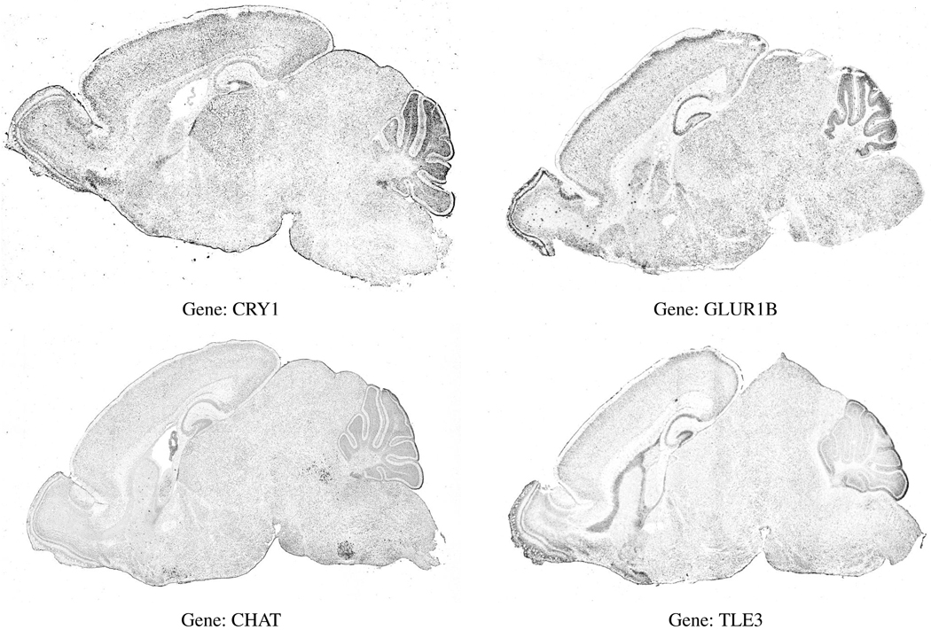
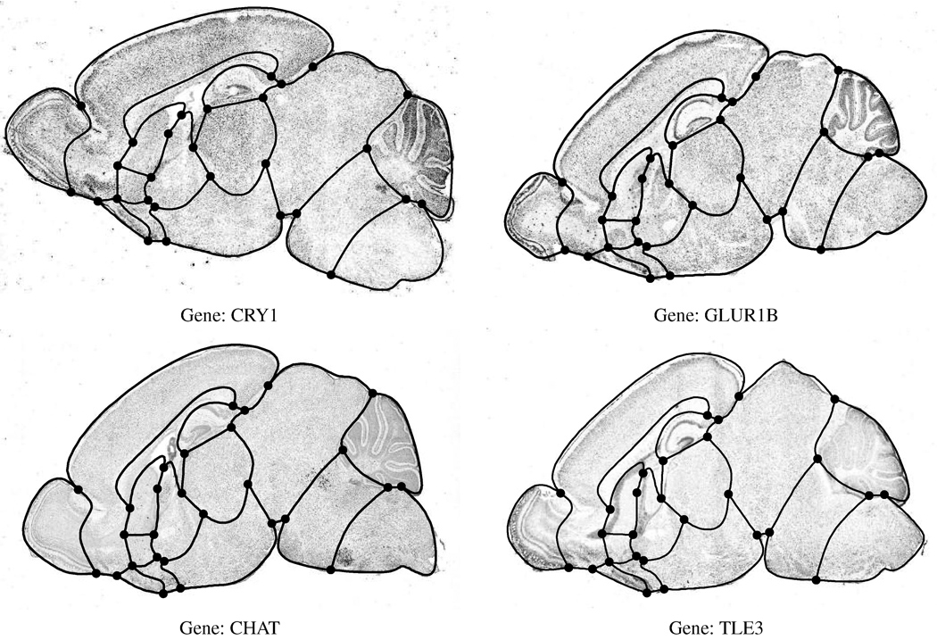
Several examples of gene expression images for one cross-section are shown in figure 1. Note that each image differs slightly due to rotations and translations induced during the data collection process, as well as the anatomical deviations between individual mice. One feature of these images is that they all exhibit common anatomical regions such as the cerebellum (the dark folded region in the upper right portion of the images).

Figure 1.

Expression images from 4 genes taken at the same approximate cross-section of the mouse brain.

1.2. Gene expression database

Given these expression images, our task is to build a database that organizes the expression data in the images into a searchable form. This database consists of eleven standard cross-sections, each corresponding to a sagittal section of particular anatomical interest. Queries to this database are of the form: "For a given cross-section, which genes have a particular expression pattern over a specific anatomical region?"

The key to answering such queries is to construct an atlas for each standard cross-section. An atlas partitions the brain into disjoint anatomical regions, each labelled by appropriate information such as its name. This labelling allows the user to pose queries in terms of named regions. To compare gene expression data from different images, the database deforms this atlas onto each image and records the expression data encoded in the image in terms of its position on the deformed atlas. This approach ensures accurate comparison of data from similar regions.

1.3. Contributions

Although there has been a great deal of work on deformable modeling and its application to anatomy (reviewed in the next section), we view this paper as making two strong, original contributions to this problem:

• We propose to use Catmull-Clark subdivision meshes as a deformable model for the mouse brain. In particular, these meshes incorporate a network of B-spline crease curves that partition the model into disjoint anatomical regions and, as result, serve as an atlas for the mouse brain. The partitioned, multi-resolution structure of these meshes allows queries comparing expression data to be performed efficiently and accurately.

• We propose a new technique for deforming these subdivision meshes to point and normal data generated from gene expression images. This method improves on a scattered data fitting technique developed by Hoppe et al.¹⁰ and incorporates a novel deformation energy term into the fitting process.

2. Subdivision meshes as deformable atlases

A range of models have been proposed to serve as deformable atlases for biological structures. For the reader interested in review of the basics of deformable modeling, we suggest two survey papers^{16, 18}. Another good reference focused more on anatomical applications is Toga’s book²³. Most deformable models consist of two basic components: a geometric representation combined with a physics-based model.

2.1. Previous deformable geometric models

One key contribution in this paper is to propose subdivision meshes as an ideal geometric representation for deformable atlases. To place our approach in perspective, we briefly review some of the other geometric representation typically used in deformable modeling.

Freeform deformations

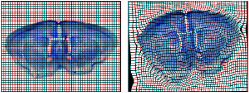
One simple approach to deformable modeling is to embed an object into a tensor product grid of points. If the grid points are interpreted as the control points for a tensor product spline, moving these control points induces a smooth deformation of the mesh (as well as the embedded object). In the case when the underlying splines are B-splines, the resulting deformations are known as freeform deformations²⁰. One standard task in this framework is to compute a deformation that maps an input object into a deformed output shape. Figure 2 shows such an example of a deformation between two brain cross-sections computed by an elastic warping algorithm due to Paul Thompson²². More recent work has developed a multi-resolution version of freeform deformations based on hierarchical B-splines²⁵.

Figure 2.

Deformation based on a uniform grid. (Thanks to Paul Thompson for this image.)

Note that one drawback of free-form deformations is that the boundaries of the embedded object do not necessarily conform to the grid lines of the deformations. For example, in figure 2, the boundary of the brain does not conform to the tensor product structure of the grid in a natural manner. As a result, freeform deformations provide only indirect control over a deformation when restricted to the boundaries of the embedded object.

Active contours

Snakes¹³, balloons⁹, and geodesic active contours⁶ are boundary-based deformable primitives that are driven to the boundaries of an object using a physic-based model. The resulting models approximate the boundaries of the object in a direct and accurate manner. More recently, T-snakes¹⁷ embed the boundary curve in a 2D tensor product grid and generates automatic topology changes in the boundary curve during fitting to the object.

T-snakes are interesting in our context in that the boundary curve is embedded in a 2D mesh which could then be used to store gene expression data. However, as was the case for freeform deformations, this 2D interior mesh has a tensor product topology that may be incompatible with the structure of internal regions in the object.

Simplex meshes

An alternative to the structured meshes used in freeform deformations and T-snakes are unstructured simplex meshes (see¹⁸ for an overview of their use in deformable modeling). Due to their lack of tensor product structure, simplex meshes are flexible enough to mesh the interior of an object while conforming to its external and internal boundaries. The main drawback with this type of representation is that regularity and smoothness of the mesh must be enforced explicitly. Another drawback is that, due to their piecewise linear nature, very fine meshes are often needed to conform accurately to curved objects.

2.2. Subdivision meshes

Given a coarse mesh M⁰, subdivision is a fractal-like process that produces a sequence of increasingly fine meshes M^k that converge to a limit mesh M^∞ following M⁰. In terms of deformable modeling, subdivision surfaces (curved 2D meshes embedded in 3D) have received only limited attention, most notably in^{14, 15}. In this paper, we propose to represent a deformable atlas as a planar subdivision mesh partitioned by an embedded network of crease curves. This explicit partitioning distinguishes our work from previous work on deformable modeling.

We focus on Catmull-Clark subdivision⁷, a subdivision scheme for quad meshes that produces provably smooth meshes in the limit. One particularly simple method for implementing Catmull-Clark subdivision is described in chapter 7 of Warren et al.²⁴. In particular, each subdivision step can be factored into two simple transformations: bi-linear subdivision, followed by centroid averaging. Under bi-linear subdivision, each quad is split into four sub-quads with new vertices placed at the midpoints of old edges and at the centroids of old faces. Centroid averaging consists of the following averaging operation:

Centoid averaging

For each vertex p in the mesh, compute the centroids of those quads that contain p. Reposition p at the centroid of these centroids.

Figure 3 illustrates this factorization applied to the initial quad mesh on the left. The result after bi-linear subdivision is shown in the middle, while the result after centroid averaging is shown on the right.

Figure 3.

Initial mesh (left), result after bi-linear subdivision (middle), result after centroid averaging (right).

To use these subdivision meshes M^k as an atlas, we must next partition these meshes into disjoint sub-meshes corresponding to distinct anatomical regions. To this end, we tagged a subset of the edges and vertices of the coarse mesh M⁰ as being crease edges and crease vertices. Taken together, these crease edges form a curve network in M⁰ that partitions M⁰ into disjoint pieces. (For subdivision surfaces, crease edges and vertices are used to introduce normals discontinuities in smooth surfaces.)

After subdivision, the image of this network of crease edges is a network of curves that partitions the limit mesh M^∞. Unfortunately, this curve network has two defects: the curve network on the limit mesh is not always smooth and the shape of this curve network depends on the position of vertices of M⁰ that do not lie on the initial crease edge network.

To address this problem, the subdivision process is now modified as follows. In the first phase (bi-linear subdivision), each crease edge is linearly subdivided into two crease edges. Next, during centroid averaging, each vertex on a crease edge is repositioned at the centroid of the midpoints of those crease edges that contain the vertex. The positions of crease vertices are left unchanged.

Now, the limit of this modified subdivision process is a smooth mesh M^∞ partitioned by a network of cubic B-spline curves that interpolate crease vertices of M⁰ and approximate the curve network formed by the crease edges in M⁰. Note that the shape of the curve network depends only on the positions of the crease vertices and crease edges in the coarse mesh M⁰.

For example, the left part of figure 4 shows an initial mesh M⁰ consisting of three quads, eight crease edges (drawn in thick lines), and one crease vertex (drawn as a round dot). The middle portion of the figure shows the result of bi-linear subdivision. Finally, the right portion of figure 4 shows the mesh M¹ generated by centroid averaging (after modification to account for crease vertices and crease edges). Figure 5 shows the sequence of meshes generated by repeatedly applying the subdivision process. Observe that the curve network defined by the eight crease edges partitions the mesh into two disjoint regions.

Figure 4.

Initial mesh with eight crease edges and a crease vertex (left), result after bi-linear subdivision (middle), result after centroid averaging (right).

Figure 5.

Initial mesh in figure 4 being subdivided two (left), three (middle) and four times (right).

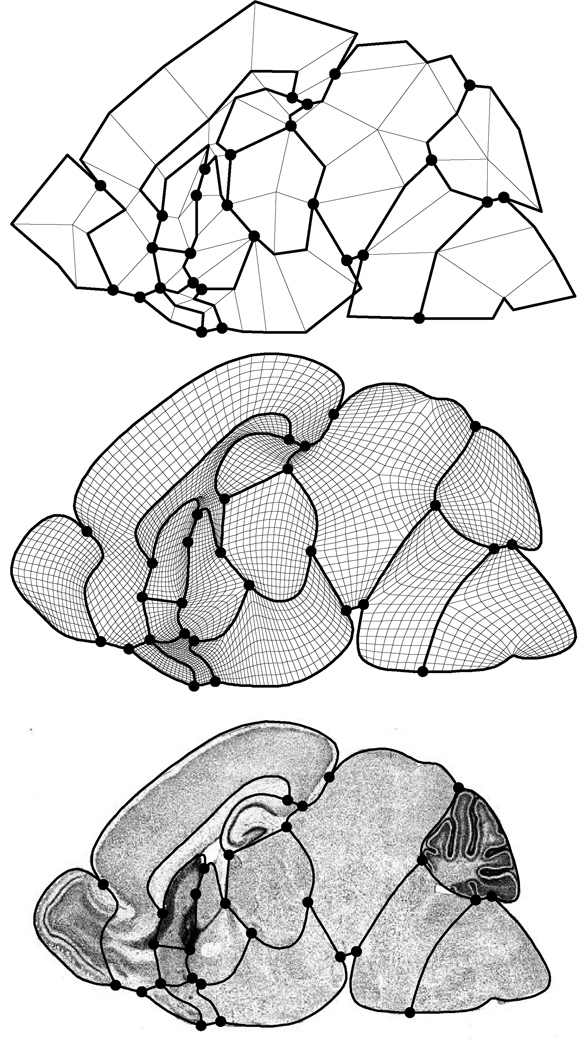
In practice, we model each standard cross-section of the mouse brain as a Catmull-Clark mesh partitioned by a network of crease curves. The top portion of figure 6 shows such a coarse mesh M⁰ for one sagittal cross-section of the mouse brain. (Crease edges are thickened; crease vertices are large dots.) The middle part of this figure shows the quad mesh M³ generated by three rounds of subdivision.

Figure 6.

Atlas at the coarsest level of subdivision (top), subdivided three times (middle), overlaid on its defining image (bottom).

Note that the crease curves partition the mesh into 15 disjoint sub-meshes. The crease edge points in M⁰ that control the shape of these curves were positioned by a mouse anatomist such that each sub-mesh corresponds to an important anatomical region of the mouse brain. The bottom portion of figure 6 shows the crease curve network and the example image used in laying out the coarse mesh M⁰. By tagging each quad in the coarse mesh M⁰ with its corresponding anatomical region, the partitioned limit mesh M^∞ serves as an atlas for this standard cross-section.

This explicit partition of our model has two substantial benefits. First, in fitting this mesh to a new expression image, we can focus our attention on the sub-problem of fitting the crease curve network to data points generated along the boundaries of anatomical regions. Second, this explicit partitioning allows queries to the associated database of gene expression data to be restricted to anatomical regions without effort.

3. Deforming a subdivision mesh onto an expression image

Given a gene expression image for a particular cross-section, our next task is to deform the atlas (i.e; subdivision mesh) for this cross-section to the image. Our solution is the standard two-step process in which the atlas is first aligned to the image using a global affine transformation and then locally fit. This global alignment accounts for rotations and translations introduced during the sectioning and imaging process. The local fitting accounts for variations in the anatomical shape of the mouse brain and tissue distortion resulting from the sectioning process.

3.1. Affine fitting using principal component analysis

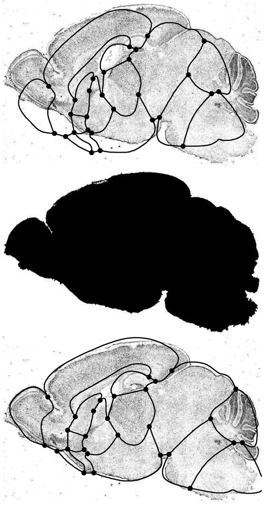
The top portion of figure 7 shows the expression image for the gene CRY1 (upper left in figure 1) overlayed with the curve network for the atlas associated with its cross-section. Our first task is to compute an affine transformation that rotates, translates and scales the atlas onto the new image. To this end, we apply a simple filter that segments the brain tissue from white background. The resulting segmentation of the gene expression image is shown in the middle of figure 7.

Figure 7.

An expression image overlayed with its undeformed atlas(top), the segmentation of the brain tissue (middle) and the atlas after affine alignment (bottom).

If the ith black pixel in this segmented image has coordinates a_i (represented as row vector), we can estimate the center and orientation of the segmented image using principal component analysis¹². The centroid c of the segmented image has coordinates $\frac{1}{n}{\displaystyle {\sum }_{i=1}^n{a}_i}$ where n is the number of black pixels. To estimate the orientation of the image, we next form the 2 × 2 covariance matrix M

$$M=\frac{1}{n}{\displaystyle \sum _{i=1}^n{(a_i-c)}^T(a_i-c).}$$

The two eigenvectors of M are orthogonal, and they describe the directions of the first and second principal variation of the data points. Together with the centroid c, these axes represent a coordinate system for the segmented image. Using a similar coordinate system computed for the atlas, we rotate and translate the atlas onto the gene expression image. The result of this deformation is shown in the bottom of figure 7.

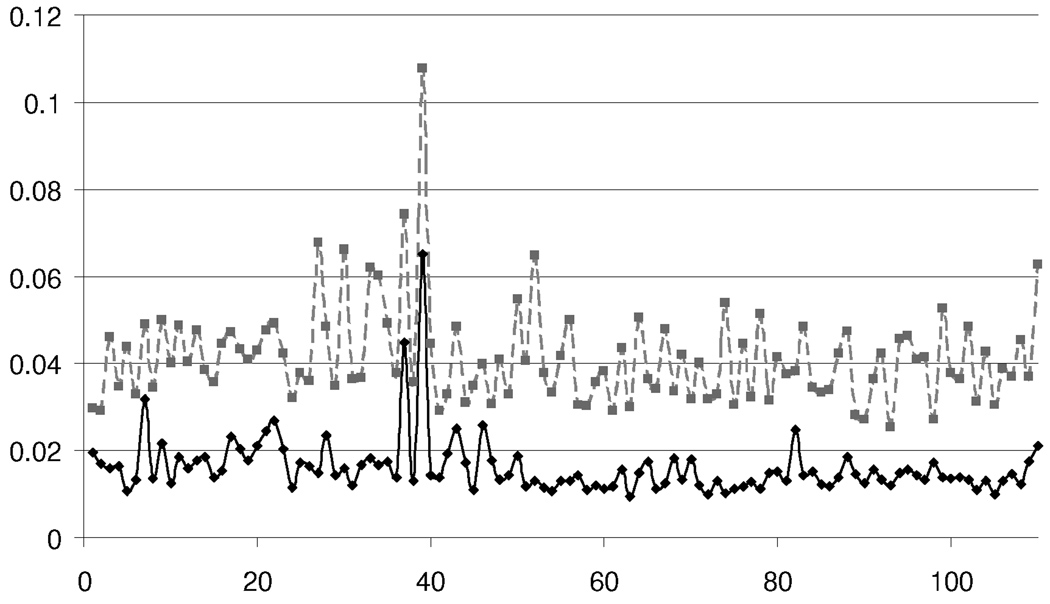
Note that this method is fast since it requires only a single pass over the gene expression image and reliable since the sagittal cross-sections have an elliptical (but non-circular) shape. The top plot in figure 8 shows an estimate of the quality of the initial alignment for 110 expression images taken at the same cross-section. The plotted error measures the area of non-overlapping portions of the aligned images versus the area of the expression image. Occasionally, poor alignments are generated due to large amounts of background noise in the expression image (corresponding to contamination during the in situ hybridization). Their high error (> 8%) is used to alert the technician collecting the images to visually examine the image and either align the image by hand or regenerate a new image.

Figure 8.

An error plot for affine fit (dotted) and affine plus local fit (solid) for 110 images taken at cross-section nine.

3.2. Local fitting using iterated least squares

Due to variations in the anatomical structure of the mouse brain, applying a global affine deformation to the coarse mesh M⁰ is not sufficient to produce a corresponding limit mesh M^∞ that accurately fits the expression image. Instead, our approach is to reposition the vertices of M⁰ and form a new subdivision mesh M̂⁰ whose associated limit mesh M̂^∞ fits the image accurately. To compute this mesh M̂⁰ we let M⁰ (x) denote the coarse mesh whose ith vertex has unknown position x_i (where x = (x₁, x₂,…)). Likewise, M^k(x) denotes the mesh resulting from subdividing M⁰ (x) k times.

Now, our goal is to compute a vector of positions x̂ such M^∞ (x̂) fits the expression image accurately while deforming M^∞ as little as possible. To this end, we construct a quadratic energy function E^k (x) of the form

$$E^k(x)=E_f^k(x)+E_d^k(x)$$

where $E_f^k(x)$ measures the fit of M^k (x) to the expression image and $E_d^k(x)$ measures the energy used in deforming M^k to M^k (x). We next construct $E_f^k(x)\text{ and }{E}_d^k(x)$.

Building the fit term

Our construction for $E_f^k(x)$ is a variant of a method for fitting a subdivision surface M^k to a set of scattered data b_j that is due to Hoppe et al.¹⁰. (Note that Hoppe’s method itself is a variant of the iterated closest point method³.) For each data point b_j, this method computes the vertex p _j of the mesh M^k that is closest to b _j and then minimizes the quadratic function

$${{\displaystyle \sum _j(b_j-p_j(x))}}^2$$

where p_j (x) is the vertex of M^k (x) corresponding to p_j.

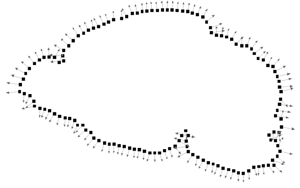
One drawback of this quadratic function is that it penalizes local translations of the subdivision mesh along flat areas of the scattered data. Our improvement to Hoppe’s method is to estimate a outward unit normal n _j for each data point b _j (see figure 9) and compute a new quadratic function of the form

$$E_f^k(x)={\displaystyle \sum _j{w}_j{(n_j\cdot (b_j-p_j(x)))}^2.}$$ (1)

where the sum runs over all data point b _j. In this model, we penalize deviation of the mesh vertices p _j (x) from the tangent lines defined by the pairs (b _j,n_j). This modified function does not penalize translations of the subdivision mesh along these tangent lines.

Figure 9.

Boundary points b_j and normals n_j for the segmented image of figure 7.

We can improve the quality of the fitting term even further by replacing Hoppe’s closest point correspondence (used in pairing b _j with p _j) by one that favors nearby points with aligned normals. For each data point b _j, we compute the closest vertex p _j of M^k whose unit normal lies within some small cone of the normal n _j. In our implementation, we restrict this search to vertices of M^k that lie within 5% of the image width of b _j and whose normals differ from n _j by at most 45°. The weight term w _j in equation 1 is simply the cosine of twice the angular difference between n_j and the normal for the chosen p _j.

Building the deformation term

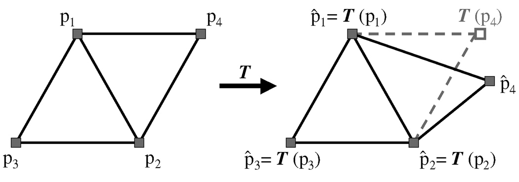
The second quadratic term $E_d^k(x)$ penalizes non-affine deformations of the mesh M^k incurred during the fitting process. To understand the structure of this term, we first focus on the simple case of deforming a triangular mesh consisting of four points p1, p2, p3, p4 into a new mesh consisting of four corresponding points p̂1, p̂2, p̂3, p̂4. (See figure 10.)

Figure 10.

Derivation of the penalty term for non-affine deformations.

Note that there exists a unique affine transformation T satisfying T(p_i) = p̂_i for i = 1,2,3. However, this transformation does not necessarily map p₄ into p̂₄. In particular, the residual T(p₄) — p̂₄ is zero if and only if there exists a single affine transformation mapping every p_i to p̂_i.

To derive an explicit penalty term based on this residual, we first observe that vertex p₄ can be expressed as an affine combination of vertices p₁, p₂, p₃ as follows:

$$p_4=\frac{1}{a_{123}}(a_{234}{p}_1+a_{134}{p}_2-a_{124}{p}_3)$$

where a_ijk denotes the unsigned area of the triangle formed by p_i, p_j, p_k. Applying T to both sides of this expression and multiplying by a₁₂₃ yields that

$$a_{123}T(p_4)=a_{234}T(p_1)+a_{134}T(p_2)-a_{124}T(p_3)$$

Applying this equation to the weighted residual a₁₂₃ (T (p₄) — p̂₄) yields a symmetric penalty term of the form

$$a_{234}{\hat{p}}_1+a_{134}{\hat{p}}_2-a_{124}{\hat{p}}_3-a_{123}{\hat{p}}_4.$$ (2)

(In practice, we divide this penalty term by the square of the area of the quad formed by p₁ , p₂, p₃, p₄ as part of normalizing the resulting energy functions.)

If we triangulate mesh M^k and its corresponding deformation M̂^k = M^k (x), taking the sum of the squares of the penalty terms generated by equation 2 for all pairs of edge adjacent triangles yields the desired energy matrix $E_d^k(x)$. As defined, the energy term $E_d^k(x)$ associated with M^k diverges as k → ∞. However, after normalizing these quadratic functions by 4^−k to account for the growth in the size of the meshes during subdivision, we have observed experimentally that the energy matrices $E_d^k(x)$ converge to a continuous energy matrix $E_d^{\infty }(x)$ for underlying continuous deformation.

Computing the deformation

To determine the desired deformation, we form the quadratic function E^k (x) (using k = 3 in our implementation) and compute the minimizer x̂ for E^k (x) using a linear solver such as conjugate gradients. We then recompute the fit term $E_f^k(x)$ from the deformed mesh M^k (x̂) and recompute the minimizer x̂ . Iterating this process several times yields a subdivision mesh M^k (x̂) that fits the boundary of the gene expression image very accurately with a minimum amount of deformation. Since the number of unknowns in this optimization process is proportional to the number of vertices in M⁰ as opposed to the number of vertices in M^k, the total fitting process takes only several seconds to run on a consumer-grade PC.

Figure 11 shows the result of applying the affine and local fitting method to the four expression images of figure 1. Note that, although the fit term currently uses only data points from the external boundary of the brain, the deformation term causes the internal anatomical boundaries of the deformed atlas to approximate the corresponding internal boundaries of the image. We are working on detecting internal boundaries of a brain image so that the deformed atlas will fit more accurately on to the internal brain features.

Figure 11.

Deformed subdivision meshes for 4 expression images at the same cross-section.

The lower plot in figure 8 shows an error plot for the deformed atlas for 110 images lying on cross-section nine. For most genes, the deformed atlas fits the expression image with less than a 3% error. For images with higher error, the technician typically improves the fit via interactive manipulation of the control points of the coarse mesh M⁰. (This level of manual interaction is acceptable since scanning a gene expression image using light microscopy takes on the order of ten minutes.)

4. Constructing and searching the database

Having deformed the atlas onto an expression image, we are now ready to add the expression data encoded in the image into the database. In this section, we discuss this process and then outline how queries to this database are generated and answered.

4.1. Adding an expression image to the database

For a particular standard cross-section, the gene expression database consists of the refined subdivision mesh M^k for the standard atlas annotated with gene expression information for each gene in the database. (In our implementation, k = 5.) The annotation for the ith gene, $G_i^k$ consists of one four-tuple of integers for each quad in the refined mesh M^k. Each of these four-tuples estimates the number of cells covered by its associated quad that exhibit one of four levels of gene expression; high, medium, low or none.

To compute $G_i^k$, we first deform the subdivision mesh M^k onto the gene’s corresponding expression image (as described in the previous section). Next, for each quad in the deformed mesh, we estimate the number of cells covered by that quad and their corresponding levels of expression. (Cell locations and their levels of expression can be computed using an image filter developed by one of the authors (Carson).) Note that the use of the deformed mesh in computing $G_i^k$ corrects for anatomical variations in individual mouse brains.

4.2. Querying the database

Having constructed the gene expression database, we can now allow users to answer queries of the following form: "For a given region of the brain, which genes have a particular expression pattern?" Using the atlas, users may specify the target region by name or by interactively painting the desired region onto the atlas. Target expression patterns can either be uniform patterns such as high, medium, low or none as well as expression patterns for a given gene.

To compute the answer to a particular query, the database compares the gene expression data for various pairs of genes. For example, if the user desires those genes whose expression patterns are similar to the ith gene in the database, the query compares all of the gene expression data $G_j^k$ to the fixed gene $G_i^k$. By computing a norm $e(G_i^k,G_j^k)$ that measures the similarity between the two expression patterns, the database then reports those genes whose norm with respect to the target gene is smallest.

In practice, we allow the user to choose between two norms, the L ₁ norm of the average gene expression level and a norm based on the χ² test (a well-known test statistic for analyzing contingency tables¹¹). For example, the L ₁ norm has the form

$$e(G_i^k,G_j^k)={\Vert \mathit{\text{av}}(G_i^k)-\mathit{\text{av}}(G_j^k)\Vert }_1$$ (3)

where $\mathit{\text{av}}(G_i^k)$ computes a vector of the average gene expression level for each quad in $G_i^k$. (High, medium, low and no expression are assigned the values 3, 2, 1, 0, respectively.) ‖v‖₁ computes the sum of the absolute values of the elements of the vector v.

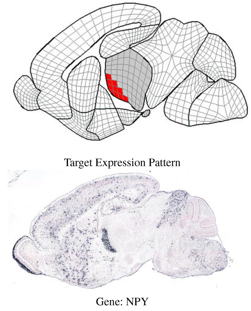
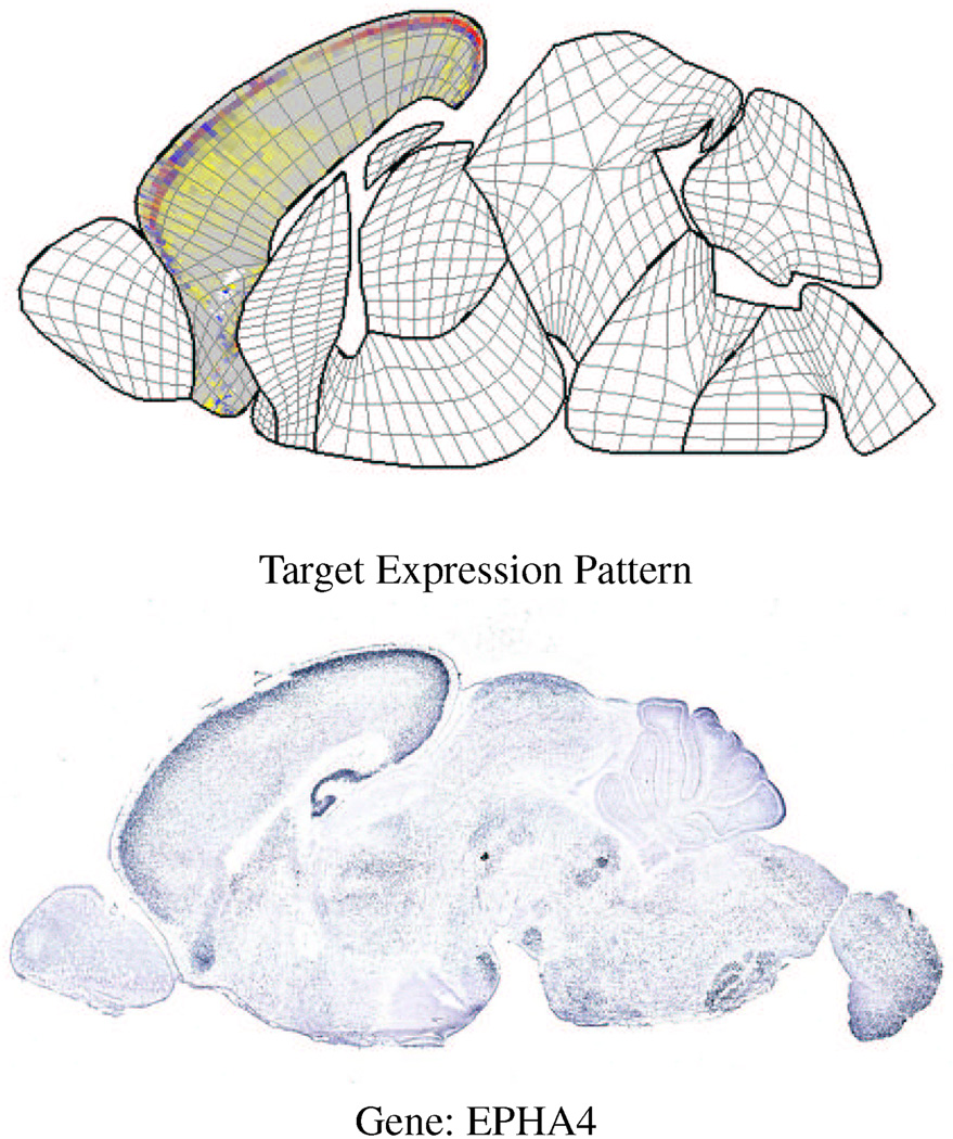
Figures 12 and 13 show examples of queries to the database at different cross-sections. In the upper part of figure 12, the user has painted a query onto the thalamus and wants to find the gene that has a higher level of expression at the lower-left corner (the darkened area). The best match is the gene NPY which has the desired expression pattern. In the upper part of figure 13, the user has selected the cortex and asked the database to find those genes whose expression pattern is similar to the gene NEUROD6 which is strongly expressed along the upper part of the cortex (as shown by the black areas in the gray quads). The best match (excluding NEUROD6) is the gene EPHA4 that exhibits a similar expression pattern along the top of the cortex. Note that this interface also allows the user to paint a query onto a sub-area of an anatomical region by selecting the corresponding quads.

Figure 12.

A query for the gene with higher expression at the lower-left corner of the thalamus at cross-section 6.

Figure 13.

A query for the gene with expression similar to that of NEUROD6 over the cortex on cross-section 11.

4.3. Accelerating the query computation

As stated, the search compares the target gene to every gene in the database at the finest level of subdivision of the atlas. By exploiting the multi-resolution structure of subdivision mesh M^k, we can substantially accelerate the search. Our technique is essentially a generalization of the multiresolution search technique proposed by Chen et al. ⁸ from rectangular images to subdivision meshes.

The key to this acceleration is to compute a multiresolution summary of the gene expression data $G_i^j$ for coarser meshes M^j where 0 ≤ j < k. For each quad q in M^j, the corresponding entry in the summary $G_i^j$ is the sum of the entries in $G_i^k$ for those children of q in M^k. Given a target expression $G_i^k$, the accelerated search first computes $e(G_i^0,G_j^0)$ for all genes j in the database and orders the genes in terms of their relative error at level 0 using a priority queue. Next, the method repeatedly extracts the gene with the smallest error from the priority queue, compares it with the target gene at a finer resolution , and inserts the gene back into the queue using the newly computed error. The search terminates when the error for the gene at the head of the priority queue has been previously computed on the fully subdivided atlas.

The search is guaranteed to return the gene with minimal error if the error function e has the property that refining the expression data for two genes increases the residual error between them monotonically; that is,

$$e(G_i^0,G_j^0)\le e(G_i^1,G_j^1)\le \cdots \le e(G_i^k,G_j^k).$$

Both L ₁ norm used in equation 3 and the χ² norm that we use have this property.

This method accelerates the search by eliminating genes that are a “bad” match at a coarser level without having to compare with these genes to the target at the fine level. Without the multi-resolution acceleration, the searches done in figures 12 and 13 took 7.76 and 7.92 seconds to find the best matches among 110 genes. (Our database currently runs on a consumer-level PC.) Using the multi-resolution method, these searches took 2.57 and 2.93 seconds, respectively, on the same computer. As the number of genes in our database grows, we intend to develop a parallel version of this search to maintain reasonable search times.

5. Future work

In the future, we will extend the proposed techniques to construct a fully 3D database of gene expressions based on a volumetric deformable atlas of the mouse brain. The brain atlas will be represented as a volumetric subdivision mesh using techniques such as the multi-linear subdivision scheme proposed in ². The subdivision mesh consists of cells (such as hexahedra) onto which gene expressions will be attached after the atlas is deformed onto a brain. In analogy to the 2D subdivision atlas in which the anatomical boundaries are captured by crease edges, the 3D subdivision mesh is partitioned into distinct volumes corresponding to each anatomical region by a network of smooth crease surfaces.

The partitioned brain atlas allows the user to pose queries to distinct anatomical regions in a fully 3D manner. To do this in an intuitive way, the user can paint queries onto 2D regions at selected cross-sections of the brain atlas (similar to the query interface in figure 12 and 13), and the selected cells of the mesh will form a 3D selection volume that can be visualized on the fly.

We are also interested in improving the quality of creased subdivision meshes. In the current 2D subdivision scheme, the mesh is only C ⁰ continuous across crease edges. We are investigating new schemes that will result in higher order continuity at those crease edges to allow a network of smooth curves embedded in a smooth surface mesh.

6. Conclusions

In summary, we believe that subdivision meshes are an ideal geometric data structure for deformable atlases. These meshes formed the core technology for a preliminary implementation of the gene expression database consisting of 1200 images for 110 genes. For the interested user, this database is fully accessible via the web at www.geneatlas.org. Our future plan is to extend the layered 2D structure of the database into a fully 3D version consisting of a single deformable atlas based on subdivision of volume meshes.

References

- 1.Alliez P, Meyer M, Desbrun M. Interactive Geometry Remeshing; SIGGRAPH ’02 Proceedings; 2002. pp. 347–354. [Google Scholar]
- 2.Bajaj C, Schaefer S, Warren J, Xu G. A subdivision scheme for hexahedral meshes. The Visual Computer. 2002;18:409–420. [Google Scholar]
- 3.Besl P, McKay N. A method for registration of 3D shapes. IEEE Transactions on Pattern Analysis and Machine Intelligence. 1992 Feb;14(2):239–256. [Google Scholar]
- 4.Carson J, Thaller C, Eichele G. A transcriptome atlas of the mouse brain at cellular resolution. Current Opinion in Neurobiology. 2002;12:562–565. doi: 10.1016/s0959-4388(02)00356-2. [DOI] [PubMed] [Google Scholar]
- 5.Carson J, Ju T, Thaller C, Christian B, Warren J, Chiu W, Eichele G. Atlasing cellular resolution gene expression in mouse brain. 2003 In preparation. [Google Scholar]
- 6.Caselles V, Kimmel R, Sapiro G. Geodesic active contours. International Journal of Computer Vision. 1997;22:61–79. [Google Scholar]
- 7.Catmull E, Clark J. Recursively generated B-spline surfaces on arbitrary topological meshes. Computer-Aided Design. 1978;16(6):350–355. [Google Scholar]
- 8.Chen JY, Bouman CA, Allebach JP. Multiscale branch and bound image database search. Storage and Retrieval for Image and Video Databases V. 1997:133–144. [Google Scholar]
- 9.Cohen L. On active contour models and balloons. Computer Vision, Graphics and Image Processing: Image Understanding. 1991;53:211–218. [Google Scholar]
- 10.Eck M, Hoppe H. Automatic reconstruction of B-spline surfaces of arbitrary topological type; SIGGRAPH ’96 Proceedings; 1996. pp. 325–334. [Google Scholar]
- 11.Hogg and Tanis. Probability and Statistical Inference. 6 edition. Prentice Hall; 2001. [Google Scholar]
- 12.Jolliffe IT. Principal Component Analysis. Springer-Verlag; 1986. [Google Scholar]
- 13.Kass M, Witkin A, Terzopoulos D. Snakes: Active contour models. International Jounal of Computer Vision. 1988;1:321–332. [Google Scholar]
- 14.Mandal C, Qin H, Vemuri BC. A New Dynamic FEM-based Subdivision Surface Model for Shape Recovery and Tracking in Medical Images. Lecture Notes in Computer Science, Proceedings of the International Conference on Medical Image Computing and Computer-Assisted Intervention (MICCAI ’98); Cambridge, MA. 1998. Oct, pp. 753–760. [Google Scholar]
- 15.Mandal C, Qin H, Vemuri BC. Dynamic Modeling of Butterfly Subdivision Surfaces. IEEE Transactions on Visualization and Computer Graphics. 2000 July-September;6(3):265–287. [Google Scholar]
- 16.McInerney T, Terzopoulos D. Deformable models in medical image analysis: a survey. Medical Image Analysis. 1996;1(2):91–108. doi: 10.1016/s1361-8415(96)80007-7. [DOI] [PubMed] [Google Scholar]
- 17.Mcinerney T, Terzopoulos D. T-Snakes: Topology adaptive snakes. Medical Image Analysis. 2000;4:73–91. doi: 10.1016/s1361-8415(00)00008-6. [DOI] [PubMed] [Google Scholar]
- 18.Montagnat J, Delingette H. Representation, Shape, Topology and Evolution of Deformable Surfaces: Application to 3D Medical Image Segmentation. Technical Report RR-3954, INRIA. 2000
- 19.Reymond A, et al. Human chromosome 21 gene expression atlas in the mouse. Nature. 2002 Dec 5;420(6915):582–586. doi: 10.1038/nature01178. [DOI] [PubMed] [Google Scholar]
- 20.Sederberg TW, Parry SR. Free-form deformation of solid geometric models; Proceedings of SIGGRAPH 86; 1986. pp. 151–160. [Google Scholar]
- 21.Stollnitz EJ, DeRose TD, Salesin DH. Wavelets for Computer Graphics: Theory and Applications. San Francisco: Morgan Kaufmann; 1996. [Google Scholar]
- 22.Thompson PM, Toga AW. A Surface-Based Technique for Warping 3-Dimensional Images of the Brain. IEEE Transactions on Medical Imaging. 1996 August;15(4):1–16. doi: 10.1109/42.511745. [DOI] [PubMed] [Google Scholar]
- 23.Toga A. Brain Warping. 1st Edition. Academic Press; 1999. [Google Scholar]
- 24.Warren J, Weimer H. Subdivision Methods for Geometric Design. Morgan-Kaufmann; 2002. [Google Scholar]
- 25.Xie Z, Farin G. Deformation with Hierarchical B-splines. Mathematical Methods for Curves and Surfaces: Oslo 2000. 2000:545–554. [Google Scholar]