A Model of the Lower Limb for Analysis of Human Movement

Abstract

Computer models that estimate the force generation capacity of lower limb muscles have become widely used to simulate the effects of musculoskeletal surgeries and create dynamic simulations of movement. Previous lower limb models are based on severely limited data describing limb muscle architecture (i.e., muscle fiber lengths, pennation angles, and physiological cross-sectional areas). Here, we describe a new model of the lower limb based on data that quantifies the muscle architecture of 21 cadavers. The model includes geometric representations of the bones, kinematic descriptions of the joints, and Hill-type models of 44 muscle–tendon compartments. The model allows calculation of muscle–tendon lengths and moment arms over a wide range of body positions. The model also allows detailed examination of the force and moment generation capacities of muscles about the ankle, knee, and hip and is freely available at www.simtk.org.

INTRODUCTION

Models of the lower limb musculoskeletal system have enabled a wide variety of biomechanical investigations. For example, a computer model of the lower limb¹³ has been used to simulate the effects of musculoskeletal surgeries such as joint replacements³⁴ and to study muscular coordination of walking,^27,32 jumping,⁴⁹ and cycling.³⁶ A more recent model of the lower limb has been used to estimate hip compression forces in children with myelomeningocele.²⁰ Other models have been used to calculate muscle forces in static positions,³⁹ estimate muscle forces during locomotion, ⁹ and study the influence hip muscles on forces in the femur during exercise and walking.²⁸

Though musculoskeletal models of the lower limb have been widely used, the experimental data on which they are based are limited. Most models have been based on two classic studies of muscle fiber lengths, physiological cross-sectional areas (PCSA), and pennation angles measured in five cadaver subjects^15,46 in combination with a model of musculoskeletal geometry ¹³ to estimate the force generation properties of lower limb muscles. Horsman et al.²¹ bypassed the inconsistency between the two sets of muscle architecture data by creating a lower limb model using muscle fiber lengths, PCSAs, and pennation angles measured in a single cadaver subject. Ward et al. recently conducted a study of lower limb muscle architecture that included 21 cadaver subjects.⁴⁴ Furthermore, Ward et al. measured sarcomere lengths from all of these muscles at known joint angles; these new data opened the possibility of creating a model that more accurately reflects muscle fiber operating lengths and force generation properties of lower limb muscles.

Our goal is to apply these new data to create a model that can reveal relationships between muscle fiber operating lengths and force generating properties. For a model to achieve this goal it must meet several criteria. First, it should be based on experimentally measured data that come from a cohesive set of subjects (i.e., not pieced together from several separate dissection studies). Second, the data set should be based on a large number of subjects to produce a generic model (as opposed to a subject specific model) that can be used to investigate general features of musculoskeletal design. Third, the model must characterize experimental measurements of moment arms and maximum moments by faithfully representing the architectural arrangements measured in the cadaver subjects.

Here, we describe a new model of the lower limb based on experimentally measured muscle architecture from 21 subjects⁴⁴ that meets these criteria. The model provides accurate representations of muscle moment arms and force generation capacities and allows detailed examination of the moment generation capacities of muscles about the ankle, knee, and hip. This model is available at www.simtk.org and can be examined and analyzed in OpenSim, a freely available biomechanics simulation application.¹¹

METHODS

We used a musculoskeletal modeling package¹² to create a generic model of a single lower limb. Bony geometry included rigid models of the phalanges, metatarsals, calcaneus, talus, fibula, tibia, patella, femur, and pelvis that were created by digitizing a set of bones from a male subject.^2,13 The bone dimensions were consistent with those of a 170 cm tall male.¹⁷ The cadavers from which muscle architecture parameters were measured⁴⁴ had an average height of 168.4 ± 9.3 cm and weight of 82.7 ± 15.2 kg.

We oriented the coordinate systems of each bone segment so that in the anatomical position the x-axis points anteriorly, the y-axis points superiorly, and the z-axis points to the right (laterally for the right leg model; Fig. 1). The calcaneus coordinate system was located at the most inferior, lateral point on the posterior surface of the calcaneus, and the toe coordinate system was located at the distal end of the second metatarsal. The talus coordinate system was located at the midpoint of the line between the apices of the medial and lateral maleoli. The tibia coordinate system was fixed in the tibia and located at the midpoint of the femoral condyles with the knee in full extension. The patella coordinate system was located at the distal pole of the patella. The femur coordinate system was located at the center of the femoral head. The pelvis coordinate system was located at the midpoint of the left and right anterior superior iliac spines (ASIS) so that the two ASISs and pubic tubercles were in the frontal (y–z) plane.² The dimensions of each bone are easily obtained from the model input files, and the locations of the coordinate systems can be transformed if desired.

FIGURE 1.

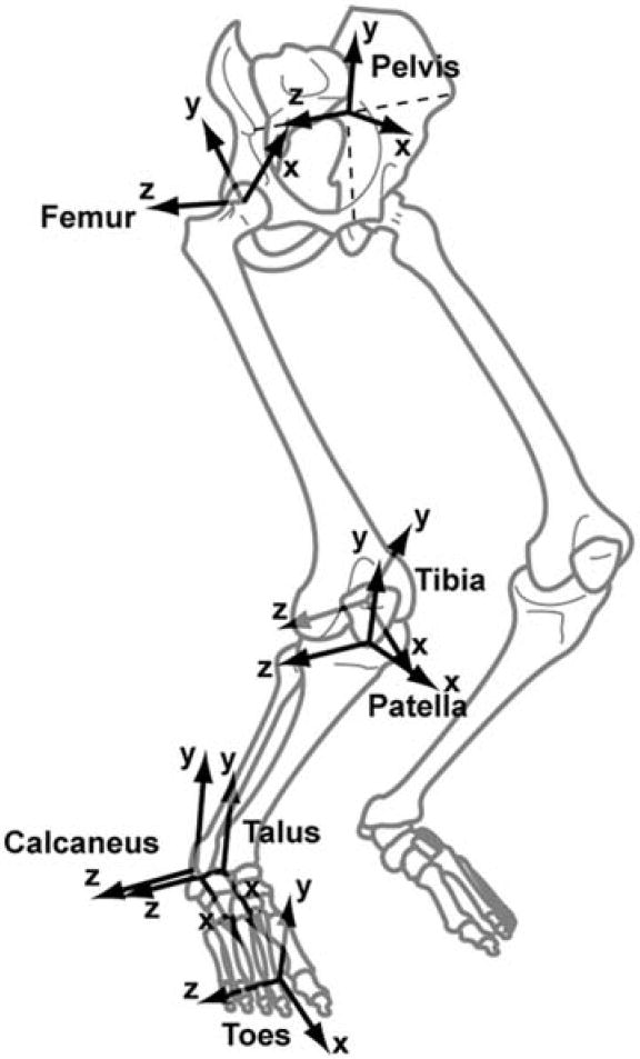
The coordinate systems of the bone segments. The systems are oriented so that when all joint angles are 0° the x-axes points anteriorly, the y-axes points superiorly, and the z-axes points to the right (laterally for the right leg). The joints in the model are defined as translations and rotations between these coordinate systems.

The model included metatarsophalangeal, subtalar, ankle, knee, and hip joints that defined translational–rotational transformations between coordinate systems. The metatarsophalangeal and subtalar joints were revolute joints, with the axes defined by Delp¹⁰ based on Inman.²² The metatarsophalangeal joint axis was rotated −8° around a vertical axis from the description by Inman and the range was −30° (extension) to 30° (flexion). The subtalar range was −20° (eversion) to 20° (inversion). The ankle was a revolute joint between the tibia and talus defined by one degree of freedom (dorsiflexion/plantarflexion), with a range of −40° (plantarflexion) to 20° (dorsiflexion).

The knee included one degree of freedom (flexion/extension) and used the equations reported by Walker et al.⁴³ for the derived translations and rotations (anterior/posterior and medial/lateral translation and internal/external and varus/valgus rotation). This model has been tested by comparing the moment arms of knee muscles to those measured in cadaver subjects.^4,7,18,40 The knee angle ranged from 0° (full extension) to 100° (flexion).

The hip was a ball and socket joint with three degrees of freedom (flexion/extension, adduction/abduction, and internal/external rotation). The joint ranges were −20° (extension) to 90° (flexion), −40° (abduction) to 10° (adduction), and −40 (external rotation) to 40 (internal rotation).

The model included 35 muscles of the lower limb (see Table 1 for list of muscles). Line segments approximated the muscle–tendon path from origin to insertion. In the case of muscles with complex geometry, such as broad attachments, multiple muscle paths were used (e.g., gluteus maximus), resulting in 44 muscle–tendon compartments. Wrapping surfaces and via points defined muscle–tendon paths that were constrained by bones, deeper muscles, or retinacula (Fig. 2).

TABLE 1.

Muscle modeling parameters.

Muscle	Abbreviation	PCSAa (cm)	Peak forcea (N)	Optimal fiber lengtha (cm)	Tendon slack lengthb (cm)	Pennation anglea (°)
Adductor brevis	addbrev	5.0	303.7	10.3	3.6	6.1
Adductor longus	addlong	6.5	399.5	10.8	13.0	7.1
Adductor magnusc,d	–	21.3	1296.9	–	–	–
Adductor magnus distal	addmagDist	–	324.2	17.7	9.0	13.8
Adductor magnus ischial	addmagIsch	–	324.2	15.6	22.1	11.9
Adductor magnus middle	addmagMid	–	324.2	13.8	4.8	14.7
Adductor magnus proximal	addmagProx	–	324.2	10.6	4.3	22.2
Biceps femoris long head	bflh	11.6	705.2	9.8	32.2	11.6
Biceps femoris short head	bfsh	5.2	315.8	11.0	10.4	12.3
Extensor digitorum longus	edl	5.7	345.4	6.9	36.7	10.8
Extensor hallucis longus	ehl	2.7	165.0	7.5	33.2	9.4
Flexor digitorum longus	fdl	4.5	274.4	4.5	37.8	13.6
Flexor hallucis longus	fhl	7.2	436.8	5.3	35.6	16.9
Gastrocnemius lateral head	gaslat	9.9	606.4	5.9	38.2	12.0
Gastrocnemius medial head	gasmed	21.4	1308.0	5.1	40.1	9.9
Gemellie	gem	–	109.0	2.4	3.9	0.0
Gluteus maximusc,g	–	30.4	1852.6	–	–	–
Gluteus maximus superior	glmax1	–	546.1	14.7	5.0	21.1
Gluteus maximus middle	glmax2	–	780.5	15.7	7.3	21.9
Gluteus maximus inferior	glmax3	–	526.1	16.7	7.0	22.8
Gluteus mediusg,f	–	36.1	2199.6	–	–	–
Gluteus medius anterior	glmed1	–	881.1	7.3	5.7	20.5
Gluteus medius middle	glmed2	–	616.5	7.3	6.6	20.5
Gluteus medius posterior	glmed3	–	702.0	7.3	4.6	20.5
Gluteus minimuse	–	–	–	–	–	–
Gluteus minimus anterior	glmin1	–	180.0	6.8	1.6	10.0
Gluteus minimus middle	glmin2	–	190.0	5.6	2.6	0.0
Gluteus minimus posterior	glmin3	–	215.0	3.8	5.1	1.0
Gracilis	grac	2.3	137.3	22.8	16.9	8.2
Iliacus	iliacus	10.2	621.9	10.7	9.4	14.3
Pectineush	pect	–	177.0	13.3	0.1	0.0
Peroneus brevis	perbrev	5.0	305.9	4.5	14.8	11.5
Peroneus longus	perlong	10.7	653.3	5.1	33.3	14.1
Peroneus tertiuse	pertert	–	90.0	7.9	10.0	13.0
Piriformise	piri	–	296.0	2.6	11.5	10.0
Psoas	psoas	7.9	479.7	11.7	9.7	10.7
Quadratus femorise	quadfem	–	254.0	5.4	2.4	0.0
Rectus femoris	recfem	13.9	848.8	7.6	34.6	13.9
Sartorius	sart	1.9	113.5	40.3	11.0	1.3
Semimembranosus	semimem	19.1	1162.7	6.9	37.8	15.1
Semitendinosus	semiten	4.9	301.9	19.3	24.5	12.9
Soleus	soleus	58.8	3585.9	4.4	28.2	28.3
Tensor fascia lataee	tfl	–	155.0	9.5	45.0	3.0
Tibials anterior	tibant	11.0	673.7	6.8	24.1	9.6
Tibialis posterior	tibpost	14.8	905.6	3.8	28.2	13.7
Vastus intermedius	vasint	16.8	1024.2	9.9	10.6	4.5
Vastus lateralis	vaslat	37.0	2255.4	9.9	13	18.4
Vastus medialis	vasmed	23.7	1443.7	9.7	11.2	29.6

^aFiber lengths were normalized to an optimal sarcomere length of 2.7 μm. PCSA was calculated as volume divided by optimal fiber length. Peak force is calculated as PCSA multiplied by a specific tension of 61 N/cm². Pennation was measured directly.⁴⁴ Exceptions are designated by notations e and h.

^bTendon slack lengths were calculated by finding the value at which the fiber length measured in the cadaver matched the value predicted by the model at the same joint angle for all muscles except those that crossed the ankle and semimembranosus. Muscles crossing the ankle assumed to be at a joint position of 20° of plantarflexion.

^cExperimental and model divisions of this muscle matched well, so each compartment was assigned a precise fiber length, pennation angle, and tendon slack length.

^dPCSA was only available for the entire muscle, so peak force was divided evenly between the compartments.

^ePCSA from Brand et al.⁶; fiber length form Friederich et al.¹⁵; tendon length from Delp et al.¹³

^fExperimental and model divisions of this muscle did not match well, so each compartment was assigned an average fiber length.

^gPCSA was only available for the entire muscle, so peak force was divided according to proportions used by Delp et al.¹³

^hPeak force and fiber length from Wickiewicz et al.⁴⁶; tendon length from Delp et al.¹³

FIGURE 2.

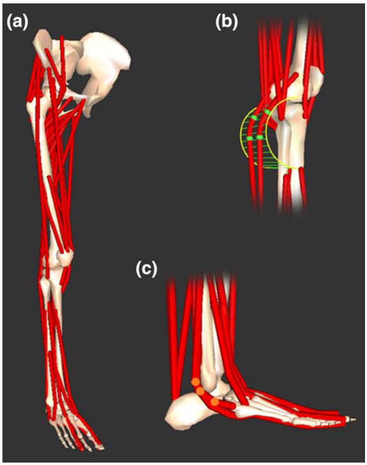
Three-dimensional model of the lower limb. (a) Bony geometry included models of the pelvis, femur, patella, tibia, fibula, talus, calcaneus, metatarsals, and phalanges. Muscle–tendon geometry used line segment paths constrained to origin and insertion points, wrapping surfaces (e.g., cylinder in b) and via points (e.g., highlighted points in c).

A Hill-type muscle model⁴⁸ characterized muscle force generation (Fig. 3). This model requires four parameters to scale generic curves for active and passive force generation of the muscle–tendon unit: optimal fiber length, maximum isometric force, pennation angle, and tendon slack length. The parameters used came from measurements made in 21 cadaver subjects by Ward et al.⁴⁴ The average age of the subjects (12 female and 9 male) was 82.5 ± 9.42 years. Six small muscles not included in the protocol of Ward et al. (gemelli, gluteus minimus, peroneus tertius, piriformis, quadratus femoris, and tensor fascia latae) were included in the model described by Delp et al.¹³; in these cases we reproduced the properties used in that earlier model.^6,13,46 The muscle–tendon parameters are summarized in Table 1.

FIGURE 3.

Hill-type model of muscle used to estimate tendon and muscle force. (a) The muscle–tendon length (l^MT) derived from the muscle–tendon geometry was used to compute muscle fiber length (l^M), tendon length (l^T), pennation angle (α) muscle force (F^M), and tendon force (F^T). (b) Tendon was represented as a non-linear elastic element. We assumed that the stain in tendon $((l^{\mathrm{T}}-l_{\mathrm{S}}^{\mathrm{T}})/l_{\mathrm{S}}^{\mathrm{T}})$ was 0.033 when muscle generated maximum isometric force $(F_{\mathrm{o}}^{\mathrm{M}})$. Muscle was represented as a passive elastic element in parallel with an active contractile element (CE). Normalized active and passive force length curves were scaled by maximum isometric force $(F_{\mathrm{o}}^{\mathrm{M}})$ and optimal fiber length $(l_{\mathrm{o}}^{\mathrm{M}})$ derived from experimental measurements for each muscle.

Optimal fiber length and pennation angle were taken from measurements made in the cadavers. For two muscles that were represented with multiple compartments, adductor magnus and gluteus maximus, the physical locations of the fiber measurements performed by Ward et al. matched the multiple muscle paths included in the musculoskeletal model. For these two muscles the model of each muscle compartment used data referenced to the location specific measurements. For gluteus medius measurement locations did not match the lines of action used in the model; thus, the average optimal fiber length and average pennation angle from the three measurements were used in the each compartment.

Maximum isometric force was calculated from measured PCSA and a specific tension of 61 N/cm² for all muscles. This value for specific tension is higher than the range of values (11–47 N/cm²) reported previously,¹⁶ and larger than the experimentally measured value for mammalian muscle of 22.5 N/cm².³⁵ It is, however, identical to the value used by Delp in an earlier model¹⁰ to scale the PCSAs reported for elderly cadavers by Wickiewicz et al.⁴⁶ Studies of age-related muscle atrophy in live, healthy subjects^24,30,47 or previously healthy subjects²⁵ (i.e., sudden accidental death) report a 19–40% decrease in PCSA in the elderly compared to the young. It is likely that there is further atrophy in the cadavers used as the basis of the model reported here due to illness or lack of physical activity in comparison to healthy elderly subjects.

Tendon slack length was based on the measured relationship between fiber length and joint position. Ward et al. measured fiber lengths and sarcomere lengths from subjects at an average position of 7° hip extension, 2° hip abduction, 0° knee flexion, and 40° plantarflexion, according to the angle conventions used here. With this information and muscle–tendon paths we computed the tendon slack length that predicted a fiber length–joint angle relationship that intersected the experimental measurement. This method worked well for all muscles except those crossing the ankle and semimembranosus.

In the ankle group, the resultant passive forces were physiologically unreasonable (i.e., passive forces were excessive). This was likely a result of a mismatch between the high degree of plantarflexion in the cadaver ankles and less extreme lengths at which the muscles were fixed. To adjust for this, tendon slack lengths for all muscles crossing the ankle were based on a joint angle of 20° plantarflexion.

In semimembranosus the fibers were very short—the shortest of all the hamstrings with an optimal length 6.9 cm⁴⁴—and the range of muscle–tendon length is large due to biarticular attachment. The tendon length calculated by the method described above predicted very long fibers with the hip flexed and the knee extended. Because semimembranosus had a large PCSA it produced passive hip extension and knee flexion moments in these positions that were excessive (i.e., much larger than experimentally measured moments). It is possible that this occurred because we do not yet fully understand how passive force properties may vary between muscles. However, since we are not yet able to justify modifying the underlying passive force model for an individual muscle we corrected this behavior by increasing tendon slack length.

The maximum isometric joint moment that a muscle can generate is the product of its maximum isometric force (as determined by the Hill-type model, assuming maximum activation) and its moment arm. We calculated the maximum isometric joint moments as a function of joint angle by summing the moments generated by all muscles that could contribute to the joint moment over a range of angles with other joints fixed. We did this for hip flexion, extension, adduction, and abduction; knee flexion and extension; and ankle dorsiflexion and plantarflexion and compared our results to an earlier model¹³ and experimental data^{1,8,23,29,31,33,38,42} of maximum isometric joint moment. In these studies isometric joint moment was measured with maximum voluntary contraction over a range of joint angles, with the other joints fixed. Most of the studies reported the results as a set of discrete points; however, Anderson et al.¹ reported a function and a set of constants to describe results for specific subgroups of subjects based on age and sex, normalized by height and weight. The results used here represent a middle-aged male scaled to match the cadaver subjects. To make the most appropriate comparisons, the joints of the model were positioned to match the position used by Anderson et al. or, in the case of adduction/abduction, other experimental results.^8,33

The model can estimate muscle forces and joint moments given any set of activation, joint positions (within the limits set on joint angles), and joint motions. Activation ranges from zero (no activation) to 1 (maximum activation). In the model, passive muscle forces are generated by muscles when they are not active and are stretched beyond their optimal length (cf. force developed by the passive element in Fig. 3). Passive joint moments were computed by summing the moments generated by all muscles that could contribute to the joint moment over a range of angles with other joints fixed and the activation of all the muscles set to zero.

RESULTS

The accuracy of the muscle paths was tested by qualitative comparison of model predicted to experimentally measured moment arms (Fig. 4).^7,18,40 The knee flexion moment arm of the biceps femoris long head peaked at 3.0 cm at 55° degrees of knee flexion. This was within the bounds of available experimental data, which showed peaks of 2.1 cm⁴⁰ and 3.0 cm⁷ at 60° and 55°, respectively. The knee extension moment arm of the model peaked at 4.7 cm at 25° of knee flexion. Though the peak extension moment arm of the model is larger than some experimental measurements,⁷ other data^14,18,40 suggest that the peak knee extension moment arm for the quadriceps is approximately 4–5 cm. Comparisons between the model and experimental results for other muscles have been made in previous publications.^3,14

FIGURE 4.

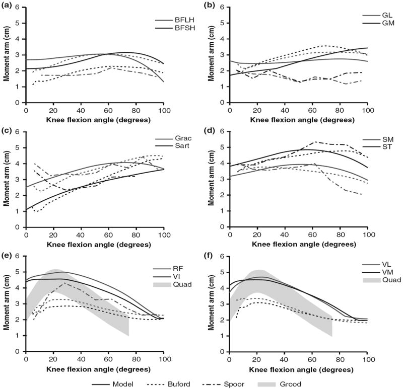
Moment arms of muscles crossing the knee in the model (solid), Buford et al.⁷ (dashed), Spoor and van Leeuwen⁴⁰ (dot-dashed), and Grood et al.¹⁸ (shaded area). Muscle moment arms are shown for (a) biceps femoris long head (BFLH) and biceps femoris short head (BFSH), (b) gastrocnemius lateralis (GL) and gastrocnemius medialis (GM), (c) gracilis (Grac) and sartorius (Sart), (d) semimembranosus (SM) and semitendinosus (ST), (e) rectus femoris (RF), vastus intermedius (VI), and grouped quadriceps (Quad), and (f) vastus lateralis (VL), vastus medialis (VM), and grouped quadriceps (Quad).

The passive joint moments estimated with the model (Fig. 5) were compared to experimental measurements.^1,37 The passive moments generated by the dorsiflexors were small (<3 Nm) over the entire range of ankle positions. The plantarflexors, however, generated more than 10 Nm of passive moment when the ankle was in 20° dorsiflexion (Fig. 5a); this occurred because the fibers of soleus, a muscle with large PCSA (Table 1), were stretched beyond their optimal lengths in dorsiflexion and generated passive forces. Medial and lateral gastrocnemius did not contribute to passive moment in this position because they are biarticular and the knee was flexed 80° to match experimental conditions. Thus, the fibers stayed shorter than optimal length even at 20° of dorsiflexion.

FIGURE 5.

Passive joint moments calculated by the model and measured experimentally. Passive joint moment was summed from all muscles crossing each joint and compared to experimental results reported by Riener et al.³⁷ and Anderson et al.¹ There are no experimental results for passive adduction/abduction moments. The joints of the model were positioned to match those used by Anderson et al. The ankle moment (a) was calculated when knee and hip flexion angles were 80° and 50°. The knee moment (b) was calculated when the hip flexion and ankle angles were 70° and 0°. The hip flexion moment (c) was calculated when the knee angle was 10°.

At the knee joint the hamstrings generated more than 10 Nm of passive flexion moment in the model and experiments (Fig. 5b). The model also predicted more than 10 Nm of passive moment generated by the knee extensors with greater than 70° of knee flexion (Fig. 5b), which is greater than passive moments measured by Anderson et al.¹ and Riener et al.³⁷ This occurred because the vasti—vastus intermedius (VI), lateralis (VL), and medialis (VM)—reached optimal fiber length at 32°, 36°, and 34°, respectively, and generated passive force as they are stretched beyond this position. This behavior may be a symptom of altered passive properties of the vasti compared to other muscle groups or complex fiber arrangements that are not captured by the lumped parameter model of muscle (Fig. 3) because the model assumes all fibers are the same length.^5,19,41

The hip flexors produced only a small amount of passive joint moment at 20° of extension, less than 5 Nm (Fig. 5c), which is less than passive moment measured by Anderson et al.¹ and Riener et al.³⁷ This occurred because the hip flexors only slightly exceed optimal fiber length in hip extension (the largest contributors to passive moment, psoas, adductor longus, and iliacus only reach 1.2 normalized fiber lengths) and have small PCSAs compared to the hip extensors. The passive hip flexion moment also includes contributions from the hip ligaments, which are not included in the model. The extensors exceed 100 Nm of passive moment at 75° of hip flexion due to large fiber excursions and high PCSAs. The model predicts a more rapid increase in passive hip extension moment than Anderson et al.¹ measured, but the scale is comparable. Riener et al.³⁷ measured comparatively very little hip extension moment (<40 Nm at 90°).

Maximum isometric joint moments for ankle dorsiflexors and plantarflexors were compared both to an earlier model and to experimental results over the range of −30° to 20° dorsiflexion (Fig. 6) with the knee flexed 80°. The predicted ankle dorsiflexion moment (peak 47 Nm at −7°) was consistent with experimental results^1,29 (peaks of 38 and 48 Nm at −16° and −10°, respectively) and the earlier model¹³ (peak 42 Nm at −2°). The ankle plantarflexion moments predicted (peak 215 Nm at 7°) showed the greatest deviation from experimental values^1,38 (peaks of 156 and 170 Nm at 20° and 15°, respectively) and the earlier model¹³ (peak of 165 Nm at 15°) of any muscle groups. Optimal fiber lengths measured in the ankle plantarflexors by Ward et al.⁴⁴ were significantly longer than values reported by Wickiewicz et al.⁴⁶ meaning that in high degrees of plantarflexion fibers did not deviate as much from optimal length and maintained force output. This resulted in a less dramatic decrease in ankle plantarflexion moment in the plantarflexed position.

FIGURE 6.

Maximum isometric ankle moments over a range of ankle angles. Dorsiflexion moments and angles are positive; plantarflexion moments and angles are negative. The moments estimated with the model were compared to a previous model described by Delp et al.¹³ and experimental data reported by Anderson et al.,¹ Marsh et al.,²⁹ and Sale et al.³⁸ The gray region indicates one standard deviation of the data reported by Anderson et al.¹

The ankle antagonist groups illustrate how structural differences result in varied functional output. The dorsiflexors—extensor digitorum longus, extensor hallucis longus, and tibialis anterior—have longer fibers than their antagonists—gastrocnemius lateral head, gastrocnemius medial head, and soleus (Table 1). As a result, the fibers of the dorsiflexors are shortened and stretched relative to optimal length less, so they produce a more consistent force and moment over the ankle range of motion (Fig. 6). The plantarflexors, however, have larger PCSAs and shorter fibers and thus produce greater peak moment and more variation relative to ankle angle.

Maximum isometric joint moments for knee flexors and extensors were compared to both an earlier model and to experimental results over the range of 0° to 100° knee flexion (Fig. 7). The knee moment was calculated when the hip flexion and ankle angles were 70° and 0°, respectively. The model prediction for knee flexion moment (peak of 122 Nm at 48°) was similar to experimental results^1,31 (peaks of 112 and 91 Nm at 28° and 30°, respectively) and an earlier model¹³ (peak of 123 Nm at 66°). The knee extensor muscle group was consistent with experimental results^1,42 near full extension, but peaked early (210 Nm at 36°) whereas the experimental measurements did not peak until 68° (212 Nm) and 60° (240 Nm). The knee extensors reached both optimal fiber length and peak moment arm at less than 40° of flexion (Figs. 4e and 4f). The combination of increasing fiber length and decreasing moment arm with knee flexion greater than 40° created a rapid decrease in active moment and increase in passive moment generation, resulting in a cumulative decrease in total moment generation.

FIGURE 7.

Maximum isometric knee moments over a range of knee angles. Flexion moments and angles are positive; extension moments are negative. The moments estimated with the model were compared to a previous model described by Delp et al.¹³ and experimental data reported by Anderson et al.,¹ Murray et al.,³¹ and Van Eijden et al.⁴² The gray region indicates one standard deviation of the data reported by Anderson et al.¹

Maximum isometric joint moments for hip flexors and extensors were compared to both an earlier model and to experimental results over the range of −20° to 90° hip flexion (Fig. 8). The hip flexion moment was calculated when the knee angle and adduction angle were 10° and 0°, respectively. The hip flexors generated a peak moment of 110 Nm at 18°. Inman et al. reported a peak of 105 Nm at 40°. Anderson et al. reported peak moment at −20° due to a high passive contribution, which our model did not predict (Fig. 5c). Predicted hip extension moments were similar to experimental results from Anderson et al. in extended and moderately flexed positions, but deviated with greater than 40° hip flexion. Anderson et al. reported increasing extension moment at increasing flexion angle while our model predicted that extension moment decreases as fibers stretch past optimal length and moment arms shorten. Waters et al.⁴⁵ did not report a large increase in extension moment in deep flexion and reported smaller values overall.

FIGURE 8.

Maximum isometric hip flexion moments over a range of hip flexion angles. Flexion moments and angles are positive; extension moments and angles are negative. The moments estimated with the model were compared to a previous model described by Delp et al.¹³ and experimental data reported by Anderson et al.,¹ Inman et al.,²³ and Waters et al.⁴⁵ The gray region indicates one standard deviation of the data reported by Anderson et al.¹

Maximum isometric joint moments for hip adductors and abductors were compared to an earlier model and to experimental results over a range of −40° to 10° hip adduction (Fig. 9). The hip adduction moment was calculated when the hip flexion and knee angles were 60° and 90°, respectively. Our model predicted a peak adduction moment of 143 Nm when abducted 10°. Cahalan et al.⁸ found a peak adduction moment of 107 Nm when abducted 20°, with decreasing moment approaching the anatomical position. The model predicted a peak abduction moment generation of 127 Nm in the abducted position, which decreased as moment arms shrank with increasing adduction. Cahalan et al. and Olson et al.³³ measured peak abduction moments of 108 and 103 Nm, respectively, at the adducted position.

FIGURE 9.

Maximum isometric hip adductor moments over a range of hip adduction angles. Adduction moments and angles are positive; abduction moments and angles are negative. The moments estimated with the model were compared to a previous model described by Delp et al.¹³ and experimental data reported by Cahalan et al.⁸ and Olson et al.³³

DISCUSSION

In this study, we created a model that predicts the fiber lengths and forces of muscles based on a robust data set of experimentally measured architecture. The model can be used to examine the interplay between moment arms and architecture to evaluate the variation in muscle forces and joint moments over a wide range of body positions. The model is available for public evaluation, refinement, and application (download at www.simtk.org).

The model derives much of its significance from the architecture on which it is based. Most existing models have been based on architecture measured 30 years ago in five cadavers mixed from two separate studies by Wickiewicz et al.⁴⁶ and Friederich and Brand.¹⁵ There is some disagreement between the two data sets, but small sample sizes preclude meaningful statistical analysis. The previous studies did not include measurements of sarcomere length, which compromises the accuracy of the reported optimal fiber lengths and necessitates rough estimation of tendon lengths. The data set used in this model came from 21 cadavers and included measurement of the sarcomere length of each muscle at a known body position. Ward et al. found longer fiber lengths in the knee extensors, knee flexors, and ankle plantarflexors, and shorter fiber lengths in the ankle dorsiflexors compared to the previous data sets. These differences have a profound impact on the musculoskeletal model because muscle force generation properties are driven by their architectural properties.²⁶

The maximum isometric joint moments predicted by the model do not exactly match experimental measurement of joint moments. It would be possible to obtain a much closer fit to experimental joint moments by varying parameters such as tendon slack lengths or PCSAs to tune the model. This would, however, sacrifice one of the strengths of the model: that it is based on a cohesive set of experimentally measured data.

There are some limitations of the model that should be considered. There are several, relatively small, muscles that were modeled based on parameters measured in older studies (gemelli, gluteus minimus, peroneus tertius, piriformis, quadratus femoris, and tensor fascia latae). However, these muscles make small contributions to the overall joint moment and are not likely to alter simulation results of joint function.

The model represents the moment generation properties of the included muscles over the ranges of −30° to 20° ankle dorsiflexion, 0° to 100° knee flexion, −20° to 90° hip flexion, and −40° to 10° hip adduction. If it is used outside these ranges, accuracy may be reduced. Knee extensors deviate from experimental results at higher flexion angles: total moment is decreased and passive moment is increased. This could imply that the single path, lumped parameter model is not sufficient for capturing the behavior of these muscles. The fibers of these larger muscles may, in fact, be distributed over a range of lengths, leading to a more gradual change in maximum force output with knee flexion.^5,19,41 If a user is particularly interested in high knee flexion applications or the high passive forces create problems in simulation the tendons of the vasti and rectus femoris may need to be lengthened.

Tendon lengths of the muscles that cross the ankle had to be adjusted from the value derived from the cadaver ankle angle. Since all muscles on either side of the joint showed non-physiological behavior prior to adjustment we suspect that the severe angle of plantar flexion measured in the cadavers did not represent the joint position at which the muscles were fixed. We accounted for this with a systematic adjustment to all ankle muscles based on a reduced plantarflexion angle, which produced reasonable results while maintaining an unambiguous link to experimental measurements.

The tendon length of semimembranosus also had to be adjusted. As with the ankle muscles, results here provide an example of how models can help us examine the assumptions we make about the links between measurement and function. The experimental measurements of sarcomere length in semimembranosus indicated that this muscle is near optimal length when hip and knee joints are neutral.⁴⁴ Thus it is no surprise that—with a moment arm that is consistent with experimental measurements—the model predicts the fibers will be stretched far beyond optimal length when the hip is flexed. The fact that the resulting passive joint moment is so inconsistent with experimental measurements suggests that there may be a flaw in our passive force model for this muscle, which we assumed to be the same for all muscles. This demonstrates that though our model and the measurements made by Ward et al. are important steps forward in our understanding of muscle structure and function there is still much to be learned.

References

- 1.Anderson DE, Madigan ML, Nussbaum MA. Maximum voluntary joint torque as a function of joint angle and angular velocity: model development and application to the lower limb. J Biomech. 2007;40:3105–3113. doi: 10.1016/j.jbiomech.2007.03.022. [DOI] [PMC free article] [PubMed] [Google Scholar]
- 2.Arnold AS, Asakawa DJ, Delp SL. Do the hamstrings and adductors contribute to excessive internal rotation of the hip in persons with cerebral palsy? Gait Posture. 2000;11:181–190. doi: 10.1016/s0966-6362(00)00046-1. [DOI] [PubMed] [Google Scholar]
- 3.Arnold AS, Blemker SS, Delp SL. Evaluation of a deformable musculoskeletal model for estimating muscle-tendon lengths during crouch gait. Ann Biomed Eng. 2001;29:263–274. doi: 10.1114/1.1355277. [DOI] [PubMed] [Google Scholar]
- 4.Arnold AS, Salinas S, Asakawa DJ, Delp SL. Accuracy of muscle moment arms estimated from MRI-based musculoskeletal models of the lower extremity. Comput Aided Surg. 2000;5:108–119. doi: 10.1002/1097-0150(2000)5:2<108::AID-IGS5>3.0.CO;2-2. [DOI] [PubMed] [Google Scholar]
- 5.Blemker SS, Delp SL. Rectus femoris and vastus intermedius fiber excursions predicted by three-dimensional muscle models. J Biomech. 2006;39:1383–1391. doi: 10.1016/j.jbiomech.2005.04.012. [DOI] [PubMed] [Google Scholar]
- 6.Brand RA, Crowninshield RD, Wittstock CE, Pedersen DR, Clark CR, van Krieken FM. A model of lower extremity muscular anatomy. J Biomech Eng. 1982;104:304–310. doi: 10.1115/1.3138363. [DOI] [PubMed] [Google Scholar]
- 7.Buford WL, Jr, Ivey FM, Jr, Malone JD, Patterson RM, Peare GL, Nguyen DK, Stewart AA. Muscle balance at the knee–moment arms for the normal knee and the ACL-minus knee. IEEE Trans Rehabil Eng. 1997;5:367–379. doi: 10.1109/86.650292. [DOI] [PubMed] [Google Scholar]
- 8.Cahalan TD, Johnson ME, Liu S, Chao EY. Quantitative measurements of hip strength in different age groups. Clin Orthop Relat Res. 1989;246:136–145. [PubMed] [Google Scholar]
- 9.Crowninshield RD, Brand RA. A physiologically based criterion of muscle force prediction in locomotion. J Biomech. 1981;14:793–801. doi: 10.1016/0021-9290(81)90035-x. [DOI] [PubMed] [Google Scholar]
- 10.Delp SL. Ph.D., Department of Mechanical Engineering. Stanford, CA: Stanford University. 1990. Surgery Simulation: A Computer Graphics System to Analyze and Design Musculoskeletal Reconstructions of the Lower Limb. [Google Scholar]
- 11.Delp SL, Anderson FC, Arnold AS, Loan P, Habib A, John CT, Guendelman E, Thelen DG. OpenSim: open-source software to create and analyze dynamic simulations of movement. IEEE Trans Biomed Eng. 2007;54:1940–1950. doi: 10.1109/TBME.2007.901024. [DOI] [PubMed] [Google Scholar]
- 12.Delp SL, Loan JP. A graphics-based software system to develop and analyze models of musculoskeletal structures. Comput Biol Med. 1995;25:21–34. doi: 10.1016/0010-4825(95)98882-e. [DOI] [PubMed] [Google Scholar]
- 13.Delp SL, Loan JP, Hoy MG, Zajac FE, Topp EL, Rosen JM. An interactive graphics-based model of the lower extremity to study orthopaedic surgical procedures. IEEE Trans Biomed Eng. 1990;37:757–767. doi: 10.1109/10.102791. [DOI] [PubMed] [Google Scholar]
- 14.Delp SL, Ringwelski DA, Carroll NC. Transfer of the rectus femoris: effects of transfer site on moment arms about the knee and hip. J Biomech. 1994;27:1201–1211. doi: 10.1016/0021-9290(94)90274-7. [DOI] [PubMed] [Google Scholar]
- 15.Friederich JA, Brand RA. Muscle fiber architecture in the human lower limb. J Biomech. 1990;23:91–95. doi: 10.1016/0021-9290(90)90373-b. [DOI] [PubMed] [Google Scholar]
- 16.Fukunaga T, Roy RR, Shellock FG, Hodgson JA, Edgerton VR. Specific tension of human plantar flexors and dorsiflexors. J Appl Physiol. 1996;80:158–165. doi: 10.1152/jappl.1996.80.1.158. [DOI] [PubMed] [Google Scholar]
- 17.Gordon CC, Churchill T, Clauser CE, Cradtmillser B, McConville JT, Tebbets I, Walker RA. 1988 Anthropometric Survey of U.S. Army Personnel: Methods and Summary Statistics. Natick, MA: United States Army Natick Research, Development, and Engineering Center; 1989. [Google Scholar]
- 18.Grood ES, Suntay WJ, Noyes FR, Butler DL. Biomechanics of the knee-extension exercise. Effect of cutting the anterior cruciate ligament. J Bone Joint Surg Am. 1984;66:725–734. [PubMed] [Google Scholar]
- 19.Herzog W, Hasler E, Abrahamse SK. A comparison of knee extensor strength curves obtained theoretically and experimentally. Med Sci Sports Exerc. 1991;23:108–114. [PubMed] [Google Scholar]
- 20.Horsman MDK. Ph.D., Department of Engineering Technology. Enschede, The Netherlands: University of Twente. 2007. The Twente Lower Extremity Model: Consistent Dynamic Simulation of the Human Locomotor Apparatus. [Google Scholar]
- 21.Horsman MDK, Koopman HFJM, van der Helm FCT, Prose LP, Veeger HEJ. Morphological muscle and joint parameters for musculoskeletal modelling of the lower extremity. Clin Biomech. 2007;22:239–247. doi: 10.1016/j.clinbiomech.2006.10.003. [DOI] [PubMed] [Google Scholar]
- 22.Inman VT. The Joints of the Ankle. Baltimore: Williams & Wilkins; 1976. [Google Scholar]
- 23.Inman VT, Ralston HJ, Todd F. Human Walking. Baltimore: Williams & Wilkins; 1981. [Google Scholar]
- 24.Klein CS, Rice CL, Marsh GD. Normalized force, activation, and coactivation in the arm muscles of young and old men. J Appl Physiol. 2001;91:1341–1349. doi: 10.1152/jappl.2001.91.3.1341. [DOI] [PubMed] [Google Scholar]
- 25.Lexell J, Taylor CC, Sjostrom M. What is the cause of the ageing atrophy? Total number, size and proportion of different fiber types studied in whole vastus lateralis muscle from 15- to 83-year-old men. J Neurol Sci. 1988;84:275–294. doi: 10.1016/0022-510x(88)90132-3. [DOI] [PubMed] [Google Scholar]
- 26.Lieber RL, Friden J. Functional and clinical significance of skeletal muscle architecture. Muscle Nerve. 2000;23:1647–1666. doi: 10.1002/1097-4598(200011)23:11<1647::aid-mus1>3.0.co;2-m. [DOI] [PubMed] [Google Scholar]
- 27.Liu MQ, Anderson FC, Pandy MG, Delp SL. Muscles that support the body also modulate forward progression during walking. J Biomech. 2006;39:2623–2630. doi: 10.1016/j.jbiomech.2005.08.017. [DOI] [PubMed] [Google Scholar]
- 28.Lu T-W, O’Connor JJ, Taylor SJG, Walker PS. Validation of a lower limb model with in vivo femoral forces telemetered from two subjects. J Biomech. 1998;31:63–69. doi: 10.1016/s0021-9290(97)00102-4. [DOI] [PubMed] [Google Scholar]
- 29.Marsh E, Sale D, McComas AJ, Quinlan J. Influence of joint position on ankle dorsiflexion in humans. J Appl Physiol. 1981;51:160–167. doi: 10.1152/jappl.1981.51.1.160. [DOI] [PubMed] [Google Scholar]
- 30.Morse CI, Thom JM, Birch KM, Narici MV. Changes in triceps surae muscle architecture with sarcopenia. Acta Physiol Scand. 2005;183:291–298. doi: 10.1111/j.1365-201X.2004.01404.x. [DOI] [PubMed] [Google Scholar]
- 31.Murray MP, Gardner GM, Mollinger LA, Sepic SB. Strength of isometric and isokinetic contractions: knee muscles of men aged 20 to 86. Phys Ther. 1980;60:412–419. doi: 10.1093/ptj/60.4.412. [DOI] [PubMed] [Google Scholar]
- 32.Neptune RR, Kautz SA, Zajac FE. Contributions of the individual ankle plantar flexors to support, forward progression and swing initiation during walking. J Biomech. 2001;34:1387–1398. doi: 10.1016/s0021-9290(01)00105-1. [DOI] [PubMed] [Google Scholar]
- 33.Olson VL, Smidt GL, Johnston RC. The maximum torque generated by the eccentric, isometric, and concentric contractions of the hip abductor muscles. Phys Ther. 1972;52:149–158. doi: 10.1093/ptj/52.2.149. [DOI] [PubMed] [Google Scholar]
- 34.Piazza SJ, Delp SL. Three-dimensional dynamic simulation of total knee replacement motion during a stepup task. J Biomech Eng. 2001;123:599–606. doi: 10.1115/1.1406950. [DOI] [PubMed] [Google Scholar]
- 35.Powell PL, Roy RR, Kanim P, Bello MA, Edgerton VR. Predictability of skeletal muscle tension from architectural determinations in guinea pig hindlimbs. J Appl Physiol. 1984;57:1715–1721. doi: 10.1152/jappl.1984.57.6.1715. [DOI] [PubMed] [Google Scholar]
- 36.Raasch CC, Zajac FE, Ma B, Levine WS. Muscle coordination of maximum-speed pedaling. J Biomech. 1997;30:595–602. doi: 10.1016/s0021-9290(96)00188-1. [DOI] [PubMed] [Google Scholar]
- 37.Riener R, Edrich T. Identification of passive elastic joint moments in the lower extremities. J Biomech. 1999;32:539–544. doi: 10.1016/s0021-9290(99)00009-3. [DOI] [PubMed] [Google Scholar]
- 38.Sale D, Quinlan J, Marsh E, McComas AJ, Belanger AY. Influence of joint position on ankle plantarflexion in humans. J Appl Physiol. 1982;52:1636–1642. doi: 10.1152/jappl.1982.52.6.1636. [DOI] [PubMed] [Google Scholar]
- 39.Seireg A, Arvikar RJ. A mathematical model for evaluation of forces in lower extremities of the musculoskeletal system. J Biomech. 1973;6:313–326. doi: 10.1016/0021-9290(73)90053-5. [DOI] [PubMed] [Google Scholar]
- 40.Spoor CW, van Leeuwen JL. Knee muscle moment arms from MRI and from tendon travel. J Biomech. 1992;25:201–206. doi: 10.1016/0021-9290(92)90276-7. [DOI] [PubMed] [Google Scholar]
- 41.van den Bogert AJ, Gerritsen KG, Cole GK. Human muscle modelling from a user’s perspective. J Electromyogr Kinesiol. 1998;8:119–124. doi: 10.1016/s1050-6411(97)00028-x. [DOI] [PubMed] [Google Scholar]
- 42.van Eijden TM, Weijs WA, Kouwenhoven E, Verburg J. Forces acting on the patella during maximal voluntary contraction of the quadriceps femoris muscle at different knee flexion/extension angles. Acta Anat (Basel) 1987;129:310–314. doi: 10.1159/000146421. [DOI] [PubMed] [Google Scholar]
- 43.Walker PS, Rovick JS, Robertson DD. The effects of knee brace hinge design and placement on joint mechanics. J Biomech. 1988;21:965–974. doi: 10.1016/0021-9290(88)90135-2. [DOI] [PubMed] [Google Scholar]
- 44.Ward SR, Eng CM, Smallwood LH, Lieber RL. Are current measurements of lower extremity muscle architecture accurate? Clin Orthop Relat Res. 2009;467:1074–1082. doi: 10.1007/s11999-008-0594-8. [DOI] [PMC free article] [PubMed] [Google Scholar]
- 45.Waters RL, Perry J, McDaniels JM, House K. The relative strength of the hamstrings during hip extension. J Bone Joint Surg Am. 1974;56:1592–1597. [PubMed] [Google Scholar]
- 46.Wickiewicz TL, Roy RR, Powell PL, Edgerton VR. Muscle architecture of the human lower limb. Clin Orthop. 1983;179:275–283. [PubMed] [Google Scholar]
- 47.Young A, Stokes M, Crowe M. Size and strength of the quadriceps muscles of old and young women. Eur J Clin Invest. 1984;14:282–287. doi: 10.1111/j.1365-2362.1984.tb01182.x. [DOI] [PubMed] [Google Scholar]
- 48.Zajac FE. Muscle and tendon: properties, models, scaling, and application to biomechanics and motor control. Crit Rev Biomed Eng. 1989;17:359–411. [PubMed] [Google Scholar]
- 49.Zajac FE. Muscle coordination of movement: a perspective. J Biomech. 1993;26(Suppl 1):109–124. doi: 10.1016/0021-9290(93)90083-q. [DOI] [PubMed] [Google Scholar]