

Abstract
Dielectric continuum or implicit solvent models provide a significant reduction in computational cost when accounting for the salt-mediated electrostatic interactions of biomolecules immersed in an ionic environment. These models, in which the solvent and ions are replaced by a dielectric continuum, seek to capture the average statistical effects of the ionic solvent, while the solute is treated at the atomic level of detail. For decades, the solution of the three-dimensional Poisson-Boltzmann equation (PBE), which has become a standard implicit-solvent tool for assessing electrostatic effects in biomolecular systems, has been based on various deterministic numerical methods. Some deterministic PBE algorithms have drawbacks, which include a lack of properly assessing their accuracy, geometrical difficulties caused by discretization, and for some problems their cost in both memory and computation time. Our original stochastic method resolves some of these difficulties by solving the PBE using the Monte Carlo method (MCM). This new approach to the PBE is capable of efficiently solving complex, multi-domain and salt-dependent problems in biomolecular continuum electrostatics to high precision. Here we improve upon our novel stochastic approach by simultaneouly computating of electrostatic potential and solvation free energies at different ionic concentrations through correlated Monte Carlo (MC) sampling. By using carefully constructed correlated random walks in our algorithm, we can actually compute the solution to a standard system including the linearized PBE (LPBE) at all salt concentrations of interest, simultaneously. This approach not only accelerates our MCPBE algorithm, but seems to have cost and accuracy advantages over deterministic methods as well. We verify the effectiveness of this technique by applying it to two common electrostatic computations: the electrostatic potential and polar solvation free energy for calcium binding proteins that are compared with similar results obtained using mature deterministic PBE methods.
1 Introduction
Many biological molecules, such as weakly charged proteins embedded in either their normal cellular or in vitro milieu, are surrounded by water, ions and other small molecules. Both experimental measurements and theoretical results have shown that subtle and small changes in salt concentration can have a strong effect on a broad spectrum of protein properties. For instance, the stability of proteins as well the protein's association with molecules ranging from small charged peptides and drugs to larger proteins and polysaccharides at both the kinetic and thermodynamic level, can be altered by changing the salt type and concentration.1–6 We still lack a complete theoretical understanding of why increasing the salt concentration and changing the salt type can either enhance or diminish protein stability and binding to charged ligands (e.g., other charged proteins), depending upon the geometry and charge distribution of the protein or its complexes. In order to interpret this simple yet fundamental experimental observation, it will be necessary to understand the long range salt mediated electrostatic interactions and hydration effects at the molecular level of detail.
The enzymatic and catalytic activity, folding landscape, precipitation and recognition behavior of proteins can also be modulated by small changes in salt concentration.5,7–11 In a recent contribution to the literature, it has been demonstrated how changes in salt concentration can have an important role in producing more potent therapeutic vaccines consisting of cationic lipid and proteins.12 Thus, a better understanding of how non-specific and bulk salt-mediated electrostatic interactions modulate the stability, biological activity, aggregation and recognition processes involving proteins will have a significant impact in drug design efforts where the target are proteins. This will clearly be of tremendous value in biopharmaceutical applications.
Implicit solvent or dielectric continuum model-based approaches, such as the PBE, which ignore the explicit treatment of water and ions but fully account for the geometric and 3D structural details of the protein charge distribution, have already shown to be quite successful in predicting some biophysically important nonspecific salt-mediated properties such as thermodynamic and kinetic binding parameters, and stability data under low to moderate physiological salt conditions, where ion-type specific (e.g., Hofmeister effects) and hydration effects can safely ignored.13,14 In principle, the explicit solvent molecular dynamics (MD) of large-scale proteins and their complexes are capable of modeling salt-mediated electrostatic and hydration effects at the molecular level of detail with higher accuracy when compared to implicit solvent models. However, very few studies of salt effects on biomolecular properties have appeared in the literature,15 some of which are only based on simple model systems.16 This is probably due to issues concerning adequate metal ion force field parameters, the long-equilibration times required to obtain converged and reliable ion distributions surrounding large biomolecules under the appropriate salt conditions, periodic boundary condition effects,17 and other problems. Of course, in time this scenario may quickly change with the push to develop better force fields (e.g., polarizable) and enhanced sampling techniques.18 In fact, a few very elegant all-atom molecular dynamics simulations examining both salt specific and nonspecific effects on the stability and binding of small charged peptides and proteins have appeared in the past few years.15,19,20
In order to better account for conformational flexibility in both stability and binding studies of proteins and other biomolecules, it has become common practice to use MD or MCMs techniques along with the PBE to compute the thermodynamic/kinetic stability or association energetics, which entails doing at several thousands of PB calculations.21 Clearly, in one such approach, known as the MM-PBSA protocol,22 which is now being widely used in pharmaceutical companies,23 robust PBE solvers that provides both accurate and fast electrostatic or polar salvation free energy predictions are important prerequisites. It should also be pointed out that MC simulations that use a dielectric continuum model for the solvent but treat ions explicitly are very valuable, and some recent studies have appeared in the literature.24 Interestingly some of these studies lend further support to the use of the LPBE due to the good agreement between the predictions of two fundamentally different computational approaches when examining salt-dependent behavior of proteins. Of course, when studying ion distributions surrounding proteins, the more accurate MC approach should be the method of choice.
Based on the above discussion, it seems that implicit solvent based approaches such as the PBE still appear to be the best alternative when modeling non-specific salt effects in biomolecular systems given their accurate, fast prediction, and ease of use for interpreting and/or predicting pertinent salt dependent properties of biomolecules when compared to the more expensive and complex explicit solvent molecular dynamics or explicit ion/dielectric solvent MC-based molecular simulation tools. Due to the above facts, the development of faster and more accurate predictions of non-specific salt dependent electrostatic properties are still an important research endeavor, since they will provide powerful software tools for diverse applications in far reaching settings, including the pharmaceutical and biotechnology industries. With this goal in mind, here we discuss a novel implicit-solvent based LPBE approach that can deliver very accurate non-specific salt-dependent electrostatic properties, over a broad range of salt concentrations, in a single PB calculation and with very high accuracy due to the inherent properties of our MC-based algorithm.
In this work, we first provide a detailed description of the random walk-MC approach for solving the LPBE for biomolecules of arbitrary size, shape and charge distribution. The use of correlated sampling in the MC simulations and its advantages over uncorrelated sampling for solving the LPBE over a broad range of salt concentrations is presented. Next, we discuss the errors and cost in CPU time and memory of the MC-based LPBE algorithm. We then employ the MC-based LPBE approach to compute some electrostatic properties (e.g., electrostatic solvation free energy, electrostatic potential) of four different EF-hand calcium binding proteins of varying net charge. We choose these since salt-mediated electrostatic interactions are important for their stability, and calcium binding affinity behavior.14 In order to validate the proposed correlated sampling scheme, we compare the computed electrostatic properties of these important proteins over a broad spectrum of salt concentrations with similar results obtained with a robust deterministic LPBE approach (Boschitsch and Fenley, in preparation.
2 Methods
The PBE provides the electrostatic potential and other important derived quantities, such as electrostatic solvation free energies and electrostatic forces at varying ionic conditions. Thus we will specialize our discussion to these computations using the PBE as the basic electrostatic model.25,26 In the past three decades, various deterministic approaches such as boundary element,27–40 finite-difference41–51 and finite-element methods,52–57 have been reported in the literature. In this work, we focus on the novel MC based solution of the PBE and when possible make comparisons with the more mature deterministic methods.
We are interested in describing a specific computational method to solve a well-defined class of electrostatics problems of biophysical significance in various fields.58 To do this, we will begin by defining the general problem for a prototypical large biomolecule composed of many spherical atoms that is immersed in an aqueous ionic solution. In Figure 1, the jth atom is modeled as a sphere of radius, Rj, with a fixed charge of magnitude qj (in units of e, the protonic charge) located at its center, xj, and the biomolecule in question is the union of such intersecting atomic spheres. In the interior region, Gi, the dielectric constant, εi, is equal to that of the solute. Thus the electrostatic potential in the interior region of the biomolecule satisfies the Poisson equation:
Figure 1.
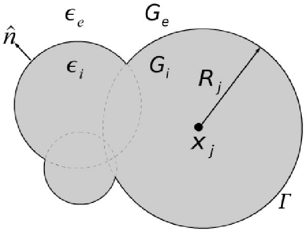
A solvated biomolecule with interior dielectric region defined by Gi and with dielectric permittivity εi. The exterior ionic solvent region, Ge, with dielectric permittivity εe. The boundary Γ separating the interior and exterior regions of the solvated biomolecules of interest is here defined by the van der Waals (vdW) surface: the union of the spherical atomic surfaces defined by the van der Waals radius of each atom j, Rj, in the molecule.
| (1) |
where ui is the normalized electrostatic potential (in units of ) in the interior region, N is the number of atoms, Δ = ∇2 is the Laplace operator, and δ(x − xj) is the Dirac delta function. The Dirac delta function is used because each atom is assumed to have its (partial) charge localized at the center of its atomic sphere.
In the exterior region, Ge, we have an aqueous ionic solution with the free ions distributed via a Boltzmann distribution, which is a standard assumption underlying the derivation of the PBE. Here the exterior dielectric constant, εe, is also assumed to be constant but equal to that of the high dielectric aqueous ionic solvent. Thus the normalized electrostatic potential (in units of ) in the exterior region containing a 1:1 salt, ue, obeys the full PBE:
| (2) |
with , κ is called the Debye-Hückel constant. Here is the ionic strength of the solvent, cb is the bulk salt concentration in moles (M), zb is the ionic valence, NA is Avogadro's number, kb is Boltzmann's constant, εe is the solvent dielectric constant, e is the protonic charge, and T is the absolute temperature of the system (in K). For small potentials, ue ≪ 1, one can linearize equation (2) to obtain the so-called LPBE:
| (3) |
In the subsequent discussion, we will only consider systems involving the LPBE.
At the biomolecule's boundary, Γ, which is defined by the van der Waals (vdW) surface, the electrostatic potential, u, and the normal component of the dielectric displacement, , are both continuous. These two boundary conditions arise from consideration of bound surface charge density at the dielectric interface. Note that for a vdW boundary, the normal vector is not uniquely defined on the intersections of spherical surfaces. However, the mathematical singularities on these curves are integrable under the condition that the molecular surface as a whole is regular.59 Due to the geometry of the molecule, possible internal cavities are treated as if they were the exterior region.60 Since we have evidence that treating these internal cavities as exterior as opposed to interior regions can affect the computed electrostatic properties in a future communication we will examine this issue in more detail, which will require some very minor algorithmic changes. Thus, the electrostatic potential inside and outside of the molecule must satisfy the following boundary conditions on Γ:
| (4) |
In addition, the potential must go to zero as we move away from the molecule:
| (5) |
We have now defined a system of elliptic partial differential equations (PDE) with appropriate boundary conditions, (1), (3), (4), and (5) whose solution gives the electrostatic potential every-where (e.g., at charge sites and in exterior domain). This system of equations, with the previously mentioned molecular geometry defines our model problem.
The fixed charges in the interior region are seen as the source of the electrostatic potential (field), and because these are modeled as point charges, they introduce singularities in the electrostatic potential. These singularities can be removed by expressing the overall electrostatic potential as the sum of a Coulombic part, which is the solution when the exterior solvent is replaced by the interior dielectric medium (i.e., the Coulombic potential generated by atomic charges in a uniform medium with interior dielectric constant throughout the whole space), and the so-called reaction field potential.
| (6) |
where
| (7) |
This explicit separation of the total electrostatic potential into two terms results in the singularity-free reaction field potential satisfying the Laplace equation in the interior region, Gi:
| (8) |
It should be noted that this decomposition of the potential is very useful, since it conveniently removes charge singularities which are inherent and problematic to some deterministic schemes. These charge singularities lead to numerical accuracy and convergence issues as well as the need to perform two LPBE computations, one as reference, as opposed to the single computation needed in the method described here. However, boundary-element and some finite-difference implementations of the LPBE39,61,61–64 also use a similar decomposition of the electrostatic potential, thus leading to more accurate solutions and CPU time gains due to the need to perform only a single computation in order to evaluate the reaction field potential.
While the quantity to be solved for in the above discussion is clearly the electrostatic potential, in most cases it is difficult to experimentally measure this quantity in a biochemical setting. However, some recent experimental studies have reported electrostatic potentials for some interesting biomolecular systems.65,66 However, there are certain scalar quantities that involve the electrostatic potential that also cannot be measured; these include the electrostatic free energy and some of its differences, such as the polar solvation and binding free energies. On the other hand, one can measure the salt dependence of the binding affinity14 and the stability of biomolecules4 using thermodynamic and kinetic techniques, and compare these results directly with similar LPBE computational predictions.
To compute the electrostatic solvation free energy, which is the electrostatic free energy change involved in transferring the solute from vacuum into the ionic solution, we need to calculate the reaction field term at the center, xj, of each atomic sphere in Gi that has a nonzero static charge, qi ≠ 0. Specifically, we must compute the electrostatic free energy change with the exterior dielectric constant, εe = εsolv (solvent) and εe = 1 (vacuum). This quantity involves only a finite number of computations for the reaction-field potential at two different exterior dielectric constants:
| (9) |
Because we are using εi = 1 in our study, the last term in equation (9) is zero because it is computed at zero salt concentration and with no dielectric discontinuity, εi = εe. Thus only the first term needs to be computed in this specific case.
2.1 Monte Carlo Solution of the Electrostatic Equations
The traditional ways to solve a system of equations like (1), (3), (4), and (5) are all based on replacing this continuous PDE system with some sort of discrete approximate system. While the details vary considerably, this is the way the finite-difference, finite-element, and boundary-element methods approach this problem.25
Once the finite-dimensional approximate systems are formed, an approximate solution is obtained by solving the resulting systems of (linear) equations. These methods of solution are all deterministic in nature, and lead to errors that are commonly studied by numerical analysts. These errors are the discretization error, caused by replacing the original, continuous, system by the appropriate deterministic approximation, and the roundoff error introduced in solving the resulting system of linear equations using floating-point arithmetic on a digital computer. Roundoff error is a function of the precision of the computer and the algorithms' design. On the other hand, discretization error can be controlled by replacing a given finite approximation with improved techniques such as “focusing”.67 This usually requires setting up a new computation with many more unknowns, and thus leads to an increase in the memory and CPU requirements for computing the solution. In this paper, we use a Monte Carlo method (MCM)68–74 to solve this same system, (1), (3), (4), and (5). Monte Carlo methods (MCMs) are fundamentally different from deterministic methods. If we have a quantity of interest, v, and we want to design a MCM to numerically determine v, we need to define a random variable, ν, that approximates v in a statistical sense. This means that the expected value  [ν] = v + β, where β is the bias (a type of MCM error), and if β = 0, then ν is called an unbiased estimator of v. Given ν, we need to have a way to statistically sample it through simulation, and then we can use our simulation to provide a MC estimate through this simulation. Since ν is a random variable, we simulate νi, i = 1, …, M, and then use
as our MCM estimate. We know its mean and can sample the variance,
, of ν̄, and so can form a confidence interval that contains the correct value with a specified probability. The width of this confidence interval is traditionally used as an a posteriori estimate of the error and is proportional to the square root of the sample variance, M−1/2σν.
[ν] = v + β, where β is the bias (a type of MCM error), and if β = 0, then ν is called an unbiased estimator of v. Given ν, we need to have a way to statistically sample it through simulation, and then we can use our simulation to provide a MC estimate through this simulation. Since ν is a random variable, we simulate νi, i = 1, …, M, and then use
as our MCM estimate. We know its mean and can sample the variance,
, of ν̄, and so can form a confidence interval that contains the correct value with a specified probability. The width of this confidence interval is traditionally used as an a posteriori estimate of the error and is proportional to the square root of the sample variance, M−1/2σν.
The errors in a MCM are qualitatively different from those in deterministic numerical methods. There are two errors in MCMs, the first is the bias, β, and has been described above. In this paper we have either β = 0 or its dependence on computational parameters will be explicitly known. It is important to note that the bias, when there is one, is the difference between the MCM's estimate and the solution to the PDE. When the estimate is unbiased, the MCM samples the solution to the PDE directly, as opposed to all the deterministic methods known, that incur a discretization error because they solve a related approximate problem, but not the actual PDE. The other error in MCMs is the so-called sampling error, and is the width of the confidence interval of the mean. As mentioned above, this is proportional to M−1/2σν, where the constant of proportionality is based on the confidence level desired in the estimate. Thus, the sampling error can be reduced by either reducing the sample variance, which is called variance reduction, or by increasing the number of samples, M. Increasing M can be achieved in many ways, such as using multiple processors, as MCMs are naturally parallel; but sampling error in MCMs scales as M−1/2. This is often viewed as a weakness of MCMs, but this sampling error is often the only significant error in a particular MCM, and reducing it does not require solving a different problem as with deterministic methods, only doing more computations on the same problem. In addition, this error is often robustly independent of other problem parameters, the problem's dimension (not important in this case), and problem geometry.
2.2 The Monte Carlo Method
The goal of this paper is to show how the MCM method we previously developed can be redeployed efficiently to solve these electrostatics problems over a broad range of salt concentrations. We deploy a correlated sampling technique, but to understand the technique we need to describe certain quantitative aspects of the underlying MCM. However, it is not appropriate to detail the technique here as it has been published in great detail elsewhere.71,72,74,75
The qualitative nature of the MC algorithm is that it creates a statistical sample of the solution of the PDE system at a point by starting a Brownian motion process at that point. Each time the Brownian motion hits the surface of the molecule, the Coulombic contribution of the potential at the hitting point is accumulated. The process then leaves the surface by either entering the molecule or the exterior region. In the interior region the process eventually hits the vdW surface again, while outside the process may return to the surface, but also can be terminated with a probability that is related to the length of the process in the exterior solvent region. In addition, this probability is related to κ: higher values of κ increase the termination probability, and thus reduce the length of the process.
Some more detail is appropriate here, but still the publication of the full algorithm71,72,74,75 should be consulted for those interested in all the algorithmic and mathematical details.
2.3 Acceleration Techniques
The technique we use requires the simulation of a complicated Brownian motion process, and specifically we need to be able to correctly sample the hitting locations of the process on the surface of the molecule. If one uses standard techniques from Brownian dynamics or stochastic differential equations, this is a complicated task. However, we can use sampling techniques based on the Walk On Spheres (WOS) method69,70,74,76,77 to accomplish this while also accelerating the computations. Since we need to only sample the hitting locations, this can be done by creating our walks in subregions where the first hitting location can be sampled exactly. Spheres are such regions, as the distribution of first hitting of a Brownian motion started anywhere within a sphere is both known and easy to sample from. In addition, since we are dealing with a problem geometry based on molecules made up of spherical atoms, the WOS technique can further take advantage of this geometry. Thus, when we start our Brownian processes we walk from point to point on the surface of spheres using WOS.
When we begin our walks, at a point in the interior, we use the WOS algorithm where our spheres are the atoms making up the molecule under consideration. There are two issues in this interior WOS scheme. The first is that often we need to walk from a point that is not the center of the sphere to a point on the sphere's surface. Fortunately, the exact first passage distribution is known via the well-known Poisson kernel. Moreover, sampling random points from the distribution defined by the Poisson kernel is very straight-forward to implement. When a new point, x, has been sampled with the Poisson kernel, there is a geometric issue: determining if x is on the surface of the molecule, Γ, or if it is on an atom's surface but still in the molecule's interior. The algorithm for answering this question is very efficient, and described elsewhere.71,72,74,75 In order to determine if a point on the surface of an atom is inside a molecule, we make use of the fact that in our model atoms are represented as spheres. The distance from a point to a sphere is equal to the distance from the point to the sphere's center less its radius. The function which computes the distance from a point to the closest atom of the molecule makes use of this fact; it will return a negative distance in response to a point which is inside of the molecule. A point which is on the surface of an atom but inside of the molecule can be recognized by noting the sign of the response from the distance function.
When the walk reaches the surface of the molecule, a decision is made as to whether one continues the walk inside or outside the molecule. The probability of returning inside is , while with probability the walk continues outside the molecule. Since εe ≫ εi, the chance of exiting the molecule is close to one. In addition to these probabilities, the location of the walker is chosen with the help of a small auxiliary sphere with radius raux. The use of the auxiliary sphere causes our MC estimate to be biased with a bias of .72 When outside the molecule, the regular WOS algorithm is used. If we are at a point outside the molecule, x, then we draw the largest sphere with center at x that is completely outside the molecule. The closure of this sphere touches the molecule at only a single point, in most cases. Then a point is chosen uniformly on this sphere to give us our new x. Since these spheres touch the molecule at only a few points at most, the WOS process can never return to the sphere in a finite number of steps. To fix this, we add a small capture region of thickness ε̄ ≪ 1, which is defined as all the points outside the molecule within distance ε̄ of the surface, Cε̄ = {x outside of the molecule ∣dist (x, Γ) ≤ ε̄}. In addition, to sample the solution to the LPBE outside the molecule, we have to either weight our sample, or terminate the walk with probability equal to this weight. Each WOS step outside the molecule occurs on a sphere with a radius, d, and this allows us to define the probability that the walker terminates with this step as .
2.4 Correlated Sampling
The second acceleration technique that we use is one that allows the simultaneous computation of the solution to the problem at all of the salt concentrations of interest. In the previous three sections we have described the random walk algorithm and the description of the probabilistic method to treat the boundary conditions. Suppose we want to compute the reaction field potential in the interior region for several different values of κ. The random walk algorithm in the interior region, as shown in Figure 2, is dependent only on the geometry, and does not depend on the value of κ. Thus the trajectories in the interior region generated for one value of κ can be reused for all other values of κ. The same thing is also true for the boundary treatment, since the probability of reentering or leaving the molecule depends only on the dielectric constant of the two regions. On the other hand, the survival probability psurv(x,y) for a random walk in the exterior region depends on the value of κ.
Figure 2.
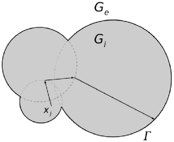
Random walk constructed by consecutive walks on spheres in the interior region, Gi.
However, for every walk in the exterior region, the radius of the WOS sphere does not depend on κ, but depends only on the geometry, as shown in Figure 3. Furthermore, we also know that the value of psurv(x,y) lies in the interval [0,1] and decreases monotonically as the value of κ increases. This means the smaller the value of κ, the longer the walk taken in the exterior region. Thus for a computation for several different values of κ, one could reuse the trajectory of the smallest nonzero κ for computing the trajectories at the other κ values. This correlated computation brings us two advantages. First, it reduces the amount of CPU time by making it possible to do an electrostatic potential computation simultaneously over a range of κ values. The second advantage relates to the nature of MCMs; by having the same reference trajectory, the estimate for different κ values will be correlated with each other. This correlation makes it possible to take the difference of two MCM estimates without introducing unacceptable levels of random error in the difference.
Figure 3.
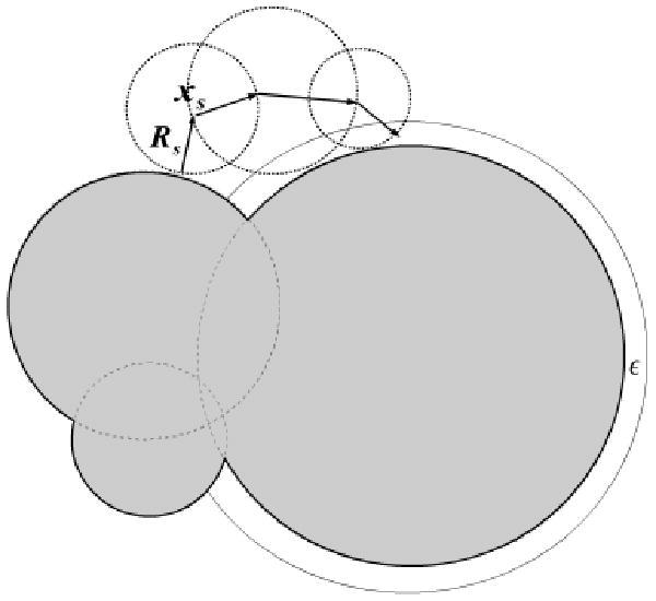
Random walk constructed by consecutive walks on spheres B(xs,Rs) in the exterior solvent region Ge. The walk will eventually come back to the boundary Γ with probability less than one. An absorbing layer with thickness ε̄ is introduced to reduce the number of walks in the exterior region.
Although the correlation algorithm can be used for the computation of electrostatic properties over a range of κ values, it is limited to only κ > 0. The reason for this is that at κ = 0 the survival probability psurv(x,y) is 1, and so walks do not terminate in the exterior. But, for κ = 0 the LPBE in the exterior turns into the Laplace equation, and one can use another exactly known probability distribution to accelerate this situation. Suppose the walk is started at the point x in Ge\B(xenc, Renc), as described in Figure 4. For this unbounded region there is a nonzero probability that the walk goes to infinity in a single step. When the walker is outside a sphere that completely encloses the molecule, the probability of walking to infinity (and termination) is Pinf. While with probability 1 − pinf a point on the surface of B(xenc, Renc) is sampled based on the Poisson kernel , as the next point of the walk. The correct Poisson kernel for exterior region is given by , where y is the point on the sphere B(xenc, Renc).
Figure 4.
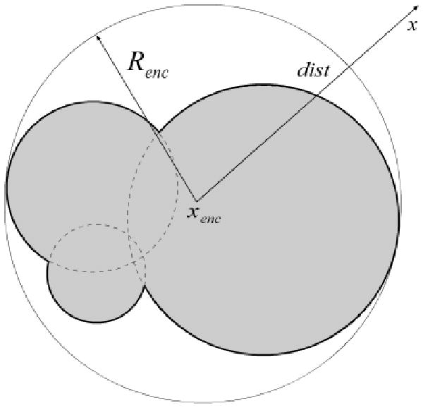
An enclosing sphere around the molecule being studied is used for the κ = 0 MC simulation. This sphere is centered at xenc and has radius Renc that is large enough to enclose the molecule. In the region outside this sphere, the electrostatic potential satisfies only the LPBE, and one can use as the survival probability for any walk starting from a distance dist from the center of the sphere.
Although we now have a new algorithm for the special case of κ = 0, the algorithm for κ ≠ 0 can also be used here. It is important to relate the κ = 0 trajectory with the κ ≠ 0 algorithm to make it possible to compute the electrostatic potential for a range of κ values which includes κ = 0, and to preserve correlation. One possible way to do this is by first generating a trajectory for the smallest nonzero κ, and to reuse that trajectory for all other values of κ, including κ = 0. Once the walk for the smallest nonzero κ terminates, the walk for κ = 0 is continued with its random walk algorithm. This ensures the correlation between the two algorithms.
2.4.1 Computational Error and Time
The statistical error of the MCM estimate, ν, (width of confidence interval) is measured in units of , where is the estimate's variance, and M is number of trajectories. Therefore, to guarantee a statistical error of δ, we have to simulate samples. This means that for a given δ, the total computational time (theoretical complexity of the algorithm) is , where t is the mean time needed for computing a single trajectory. The length of the trajectory depends on several parameters: the coefficient κ, the width of the strip near the boundary ε̄, and the radius of the auxiliary sphere, raux.
Brownian motion trajectories in the exterior region either terminate or return to the molecular surface, Γ. Thus the overall number of simulated points depends linearly on the number of boundary hits. The probability of terminating the walk depends linearly on the initial distance from the boundary in the exterior domain. This means that the average number of steps in the walk before revisiting the boundary is finite and proportional to the inverse of the initial distance: . For a given boundary strip width, ε̄, the number of steps between two consecutive boundary hits scales like log ‖ε̄‖. Our computations show that the dependence on κ is also weak, and the length of the random walk scales like O(log κ).
The terminating condition for the walk depends on κ and the distance to the boundary. The walk in the interior is done in a bounded region, while the exterior walk is done in unbounded region. This means that the length of the Brownian trajectory is dominated by the part of the trajectory in the exterior region. Thus, the CPU time is dominated by the walk in the exterior rather than by any other processes. For every walk in the exterior region one needs to find the closest boundary point and compute the distance to the boundary. In a linear search this will take time O(N), where N is the number of atoms in the molecule. In our paper we use the Approximate Nearest Neighbor (ANN) algorithm which scales as O(log(N)).? ?
2.4.2 Correlated vs Uncorrelated Random Walk Sampling
The mean μ and statistical error come from the scoring function ucoulomb, where its evaluation depends on the location of the charges and the geometry of the molecule. In uncorrelated sampling, both μ and for different values of κ are computed from independent trajectories. Therefore for an arbitrary number of trajectories, M, there is no guarantee of a monotonic behavior of μ vs κ. In this case, a plot of μ vs κ would give an oscillating curve, that would converge to a smooth curve as M → ∞. Thus it will be difficult to draw information of salt derivative of electrostatic property which is the slope of the function. On the other hand, the simulation in correlated sampling of a set of κ employs the survival probability, psurv, in all trajectories, which guarantees the monotonic behavior of μ vs κ. Therefore the salt derivative of any electrostatic properties can be computed with very high accuracy using correlated sampling.
2.5 Structure Preparation
Four calcium binding proteins of varying net charges and charge densities were selected from the RCSB database (http://www.rcsb.org) with the following PDB ids: 3ICB (net charge=-7e, surface charge density=-0.055704 ), 1EDM (net charge=- 14e, surface charge density=-0.27852 ), 3CLN (net charge=-22.5e, surface charge density=-0.17684 ) and 1PRW (net charge=-24.5e, surface charge density= -0.17525 ). Preparation of the calcium binding proteins was done following two simple protocols since in this work we are not attempting to make any comparison with experimental data, only to similar deterministic LPBE results. In both protocols missing protein side chains were not modeled and all co-factors, calcium ions and water molecules were removed from all structures prior to any further calculations.
In the first protocol hydrogen atoms were not added to the structures since we are employing a simplified formal charge model. Moreover, the structures were not subjected to any energy minimization procedure. The ionization state at physiological pH was adopted, i.e., ionized forms for side chains of Arg, Lys, Asp, Glu and C-terminus residues, and ionized forms for the His side chains. In the simplified formal charge model all atoms had zero net charge with the exception of the following atoms whose charges were assigned as follows: Arg (NH1=+0.5e, NH2=+0.5e), Lys (NZ=+1e), Asp (OD1=-0.5e, OD2=-0.5e), Glu (OE1=-0.5e, OE2=-0.5e), C-terminus (OXT=-1e), and His (ND1=0.25e, NE2=0.25e). The following Bondi-radii78 were assigned: C=1.7 Å, 0=1.4 Å, N=1.4 Å and S= 1.8Å. With the formal charge assignment, there is a significant CPU savings because the walks in MC simulation only need to be started at sites where charges are nonzero. However, since atoms with zero charges are not necessarily modeled as point charges, their geometries are still accounted for in the MC simulation. For some of the atoms that are assigned to have zero radius, the random walk is started in the same way as at other atoms.
In some of our LPBE calculations, the pdb2pqr server (http://pdb2pqr-1.wustl.edu/pdb2pqr)79 was used in order to obtain a pqr file based on the Charmm or Amber molecular mechanics force fields. In these cases the default settings of the pdb2pqr software were used. Hydrogen atoms were added to the structures and the radii and charge assigned according to the Charmm80 or Amber81 force fields.
In 3.3, the Amber force field was used to generate the charges and radii of the atoms for “hypothetical molecules” that were constructed from the initial vitamin D-dependent calcium binding protein structure (PDB id:3icb). We generated several different unphysical molecules from four 3icb molecules by stacking the 3 molecules that were shifted by 2Å in x, y, and z directions to the original 3icb molecules. We then made a spherical cut of this molecule with several different radius so that we have several molecules with globular shapes and varying size: 503, 601, 702, 800, 984, 2973, and 4257 atoms. The CPU time is geometrically dependent, thus by using the same geometry for all test cases we fix the dependence on geometry while varying the number of atoms.
2.6 Monte Carlo-Based LPBE Calculations
As in any deterministic LPBE solver, the user is required to provide an input file containing the coordinates, charge and radii for each of the atoms of the biomolecule (e.g., a pqr file obtained from the pdb2pqr software (see above)). The other usual and standard PBE parameters such as temperature of the solution, interior solute and exterior solvent dielectric constants have to be provided by the user in an input file. The specification of boundary conditions and other grid-based parameters is not necessary due to the non-grid based and stochastic nature of the MCM. The radii and charge values used in this study are given in Section 2.5, while the solvent and protein dielectric constants were 78.5 and 1, respectively. The temperature of the solution was fixed at 298 K (room temperature). The 1:1 salt (i.e., NaCl) concentration varied in the range of 0 to 1 M (0, 0.0001, 0.0002, 0.0005, 0.001, 0.002, 0.005, 0.01, 0.02, 0.05, 0.1, 0.2, 0.5, and 1M).
Some important code parameters that are intrinsic to the MC approach that need to be specified by the user are: the absorbing layer82,83 width which was set to 0.0001 Å, the auxiliary sphere radius72 which was set to 0.01 Å, and the number of trajectories, which was set to several different values depending on the problem being studied. The choices of these parameters were based on the trade off between the CPU time and the desired accuracy of the MC simulation. The optimal values of the first two parameters depend on the geometry of the molecule.
2.7 Deterministic Finite-difference vs MC LPBE Calculations
In order for any new algorithm to become mainstream and made available to the user community it is very important to validate it against different algorithms that solve the same problem. So with this goal in mind, here we compared the MC LPBE solver with results obtained with an innovative and mature deterministically-based (i.e., multi-grid finite-difference) PBE solver (Boschitsch and Fenley, in preparation). We had already established that this latter deterministic PBE solver is in very good agreement with other PBE solvers and analytical results (results not shown).
As in the MCM method, in this deterministic PBE solver only the reaction field potential is computed in the interior region, thus eliminating singularities at the charge sites and eliminating the need for a fine mesh or complications of self-energy effects in the vicinity of these sites. In the exterior region, the total potential is calculated. Here we examine the predictions of two important electrostatic properties the electrostatic potential at user specified sites and the electrostatic solvation free energies. Both of these are required in order to examine the role of electrostatic interactions in processes such as binding, folding and recognition of biomolecular systems.
The dielectric boundary separating the solute and solvent regions was the vdW surface generated by the union of spheres centered at each atom. For consistency with the MC results, no ion-exclusion region was employed. To estimate the error of the PBE calculations due to grid resolution, the calculations were repeated at the finest grid spacings of 1.5, 1.0, 0.8, 0.4, 0.2 and 0.1 Å. Our results are stable and converged for resolutions as coarse as 0.4 Å (results not shown). To strike a compromise between accuracy and efficiency, we used a fine grid spacing of 0.3 Å. The dimensions of the grid were set to three times the largest dimension of the molecule.
3 Results and discussion
3.1 Correlated vs Uncorrelated Random Walk Sampling
One of the motivations for accurately computing salt-dependent electrostatic solvation free energies resides on their use in helping experimentalists interpret salt-dependent thermodynamic stability data for moderate to highly charged biomolecules, such as certain halophilic and thermophilic proteins.13,84,85
Here we focus on an overall anionic vitamin D-dependent calcium binding protein (PDB id: 3icb), which, as shown in Figure 5, has significant negative potential over most of its surface. Note also that the calcium binding pockets, which consist of anionic Asp (D) and Glu (E) residues (a DEEE pattern at the calcium binding sites) in its surroundings generates a characteristic negative electrostatic patch near the two calcium binding sites. This characteristic potential surface patch at calcium binding sites is a general characteristic of all calcium binding proteins here studied (See Figure 5).
Figure 5.
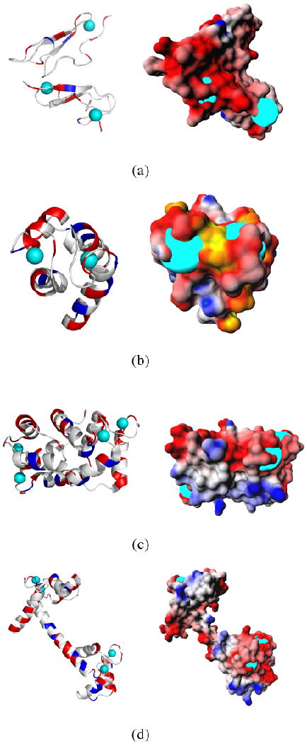
The 3D structures of four calcium binding proteins (given by their PDB ids) along with their surface electrostatic potential maps are displayed. (a) 1edm (b) 3icb (c) 1prw and (d) 3cln. The calcium ions are shown as cyan colored spheres. Note that for all four calcium binding proteins an extensive patch of negative electrostatic potential lies around the calcium binding sites, which are created by unique patterns of Asp and Glu residues. The color scheme used in these surface electrostatic potential maps is as follows: yellow is the most negative and green is the most positive. White is neutral. Red and blue represent negative and positive potentials, respectively.
In this section we examine the salt dependence of the electrostatic solvation free energy of vitamin D-dependent calcium binding protein, which has a significant salt dependent-electrostatic solvation free energy, using both the uncorrelated and correlated sampling MC approaches. Our goal here is to show the importance of using the correlated MC sampling in terms of both its CPU time and enhanced accuracy when calculating the salt-dependent electrostatic solvation free energies, , of arbitrarily complex-shaped biomolecules.
As shown in Figure 6, the electrostatic solvation free energies of the vitamin D-dependent calcium binding protein is plotted as a function of the logarithm of the NaCl concentration in the range of 0.001 M to 1 M (for a total of 14 salt concentrations). We generated 500, 1500 and 4500 trajectories for the uncorrelated MC sampling computations as opposed to 500 trajectories for the correlated sampling MC computations. As shown in Figure 6 the uncorrelated random walk sampling gives a very nonsmooth (i.e., jagged) vs log(salt concentration) curve. It is clear that this behavior is more pronounced when the number of trajectories is smaller since the fluctuation of the peaks are larger and thus the plot is more visibly jagged. These large fluctuations of are a reflection of the fact that the simulations at the different salt concentrations were carried out independently, i.e., they are uncorrelated with each other.
Figure 6.
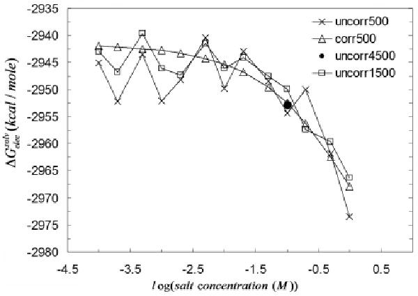
Electrostatic solvation free energy ( ) of the vitamin D-dependent calcium binding protein (PDB id:3icb) calculated using four different protocols: uncorrelated sampling with 500 trajectories at each salt concentration, uncorrelated sampling with 1500 trajectories at each salt concentration, uncorrelated sampling with 4500 iterations at each salt concentration, and correlated sampling with 500 trajectories.
It would be difficult to extract any salt derivatives of electrostatic solvation free energy at specified salt concentrations using finite-differencing techniques when the uncorrelated sampling approach is employed. This can be remedied by using a large number of trajectories. However, this approach is not practical from the CPU time point of view. On the other hand, by using the correlated sampling method, one can attain highly accurate salt-dependent electrostatic properties with a very low CPU time cost since a single PBE run is required for any user specified number of salt concentrations. In the correlated MC simulations, the survival probability of the random walk in the exterior region is independent of the geometry of the molecule. Thus with the same trajectory one can obtain energy estimates for all different salt concentrations. On the other hand, in the implementation of the uncorrelated random walk sampling, separate and independent walks are done for each of the salt concentrations. Therefore for the same level of accuracy, the CPU time for a correlated MC simulation with Nconcentration salt concentrations is on the order of Nconcentration times smaller than in the uncorrelated MC approach.
In the low salt region where the MC trajectory takes longer to complete, there are consequently larger fluctuations in the energies as reflected in Figure 6. As expected, we also observe that the uncorrelated random walk data points fluctuate around the smooth line of the correlated sampling energy values. As one increases the number of trajectories from 500 to 1500, the computed data points of for uncorrelated sampling approach to the computed curve for correlated sampling. This implies that by increasing the number of trajectories the uncorrelated random walk energies approach the smooth line generated by the correlated sampling energy curve.
Here we also computed the fluctuations of the energies relative to its normalized mean values for both types of sampling: correlated and uncorrelated. In order to get the same level of accuracy for the energies computed at 0.1 M NaCl using a correlated MC approach requires only 500 trajectories, whereas for uncorrelated MC simulation at least 4500 trajectories are necessary. This means that for this specific case, the correlated sampling gives an overall advantage of about a factor 126, which is obtained from the relationship: .
3.2 CPU Cost and Statistical Error of the LPBE MCM
As shown in section 3.1 the fluctuations of the MCM energy estimates depends on the number of trajectories employed as well as the specified range of salt concentration. It was also shown that the correlated sampling algorithm provides a significant CPU savings since the computations for a set of salt concentrations are done all in one PBE calculation. Moreover, this approach also provides a smaller statistical error for the same number of generated trajectories. In the MC simulation for the vitamin D-dependent calcium binding protein, which was done using 500 trajectories, the fluctuation (or error) of the electrostatic solvation free energy for κ = 0 is about 0.1%, which is a very small error compared to what can be attained with some deterministic PBE methods. If such a small error is not required for a particular electrostatic property being computed with MCM, one can reduce the number of trajectories and therefore save significant CPU time.
As an example, we computed the salt dependence of the electrostatic solvation free energy of calmodulin (CaM) (PDB id :3cln). The 3D structure of CaM along with its characteristic electrostatic potential map are shown in Figure 5. If one requires a very small error of 0.1% in the electrostatic solvation free energy, the MCM simulation will require 625 trajectories. On the other hand, a less stringent, but still very good level of accuracy of about 0.5% only requires 25 trajectories and takes 33 minutes to complete on a machine with a 2.8 GHz AMD Opteron 8220 Dual-Core processor.
We can obtain a significant CPU time gain on the order of 25, by simply increasing the error level from 0.1% to 0.5%, which still leads to extremely accurate values for salt-dependent electrostatic properties. Therefore it is more straightforward to control the accuracy level of electrostatic properties with our MCM as opposed to the more mature deterministic PBE methods. With deterministic PBE solvers the end-user needs to do some further analysis in order to determine the accuracy of the PBE solution.
3.3 The Dependence of CPU Time on the Size of the Biomolecule
In order for any new PBE algorithm to become mainstream in the community it is important to assess how its accuracy and CPU time scale with system size. Thus, in this section we address how the CPU time of our MCM-based PBE computation scales with the size of the biomolecular system and how this compares with the scaling of alternate deterministic PBE methods.
In this section we use an “unphysical” biophysical system in order to preserve the globularity of the hypothetical biomolecule. The requirement of using similar geometries for these unphysical molecules is done so that all molecules have the same CPU time dependence on the geometry. Thus we computed the dependence of the CPU time on the number of atoms for an unphysical toy model.
We already described how we constructed “hypothetical biomolecules” of comparable globularity but with different numbers of atoms (i.e., 503, 601, 702, 800, 984, 2973, and 4257 atoms). We evaluated how the CPU time taken in the computation of the salt dependence of the electrostatic solvation free energy of such “toy biomolecules” scales with the number of atoms.
The nature of the discretization required in deterministic finite-difference PBE solvers limits the computational domain to a bounded region. These intrinsic limitations of the popular finite-difference solvers combined with their computational box effect limits its ability to accurately compute electrostatic properties of large-scale biomolecular systems such as viruses, which can have a million or more atoms, without the need for sophisticated computer platforms.86
In our MCM algorithm the random walk done in the interior region is bounded by the molecular surface, whereas the exterior random walk is unbounded. The walk in the exterior region is terminated with the complement of its survival probability, 1 − psurv. In principle, there is no error associated with computational box effects. Because of the intrinsic nature of the MCM algorithm, the simulation time is dominated by the walk in the exterior region rather than other processes (e.g., walk in the interior region, evaluation of the Coloumbic potential). The CPU time as a function of the number of atoms for a random walk is thus O(ln(N)).
In Figure 7 we plot the CPU time as a function of the number of atoms (N) for molecules of differing sizes. As can be inferred from this figure, our results show that for molecules with a small number of atoms the CPU time per atom per trajectory follows a linear scaling while for molecules with a large number of atoms this gets closer to a logarithmic scaling. Although we compute the CPU time of the MCM for “hypothetical biomolecules”, this trend should also apply to any arbitrary and realistic biomolecule.
Figure 7.
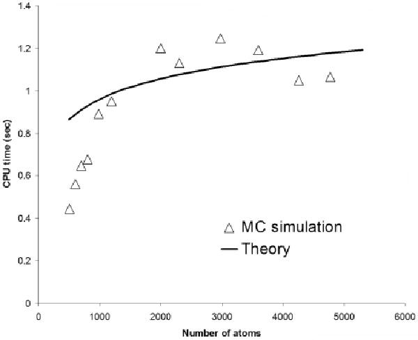
The CPU time per atom per trajectory as a function of the number of atoms of hypothetical globular-like molecules. For a small number of atoms the CPU time scales linearly with the number of atoms whereas for larger molecules the scaling approaches a logarithmic behavior.
3.4 Stochastic versus Deterministic Predictions of the Salt Dependence of the Electrostatic Solvation Free Energy of Calcium Binding Proteins
The salt dependence of the electrostatic solvation free energy of four calcium binding proteins (PDB ids: 1prw, 3cln, 1edm, and 3icb) obtained with the MCM is compared against similar finite-difference-based predictions. Based on previous results, we anticipate that the salt sensitivity of the electrostatic solvation free energies of the four calcium binding proteins will be different-given their differing charge densities. In fact, the salt dependence of the electrostatic solvation free energies are expected to be more pronounced for proteins with higher charge densities. As shown in Figure 8, our MCM results are in excellent agreement with similar deterministic PBE results, thus showing the excellent accuracy of two fundamentally different numerical solutions to the same PDE.
Figure 8.
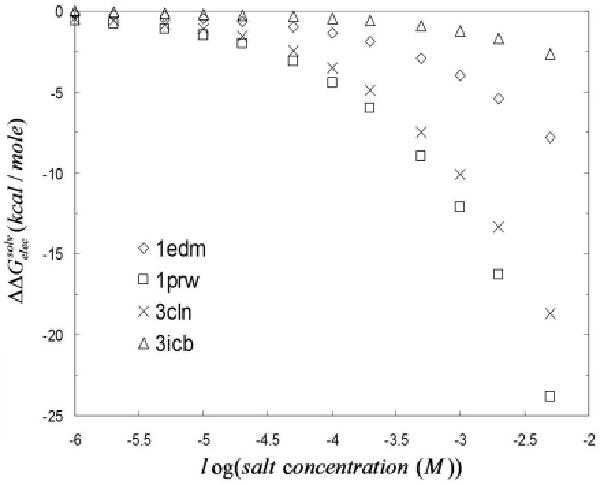
Relative electrostatic solvation free energy ( ) versus the logarithmic of the bulk 1:1 salt concentration (in M units). In the limit of zero salt concentration, the slope of the curve also tends to zero. The magnitude of the slope of the curves is larger for the calcium binding proteins with higher net charges.
Figure 8 shows the salt dependence of for all four proteins, where is the electrostatic solvation free energy at a finite salt concentration relative to that at zero salt concentration as defined by the following equation:
| (10) |
Figure 8 shows that the proteins exhibit different salt dependent behavior in the medium to high salt range. The more pronounced salt sensitivity of for calmodulin (PDB id: 1prw) is a reflection of its larger net charge (charge density).
Figure 9 shows the limiting behavior of the electrostatic solvation free energy w.r.t log(salt concentration) computed with MCM and the deterministic PBE method. In the limit of zero salt concentration, the salt derivative of the electrostatic solvation free energy of calmodulin (PDB id:3cln) computed with both codes converges to zero. This also shows that the deterministic energy result falls well within the 95% confidence interval of similar MCM energies. As a comparison we also plot the salt derivative of the electrostatic solvation free energy w.r.t κ at extremely low salt concentration. Figure 10 shows that both PB codes predict comparable salt-derivatives in the limit of κ = 0 (differing by 20%). For the other 3 calcium binding proteins, smaller differences were observed (results not shown). The derivation of the expressions for the limiting behavior of the two different salt derivatives of the electrostatic solvation free energies is given in the Appendix.
Figure 9.
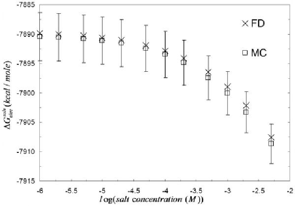
Comparison of the salt dependence of the electrostatic solvation free energy ( ) of calmodulin (PDB id: 3cln) obtained with two independent and very distinct PB solvers: MC and deterministic. The graph shows that the deterministic results fall well within the 95% confidence interval of MC energy values at all salt concentrations. Moreover, in the limit of zero salt concentration, the salt derivative of is equal to zero for both deterministic and LPBE MCM.
Figure 10.
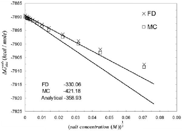
The behavior of the salt derivative of (w.r.t κ) at the limit of κ = 0. The plot shows that both deterministic and MCM predict a comparable salt behavior in an extremely low salt regime.
3.5 Calcium Binding Site Potentials
It is well established that the electrostatic environment plays a key role in metal binding to proteins, including calcium binding proteins.87 Locating potential metal binding sites in proteins and nucleic acids using implicit solvent models, such as the PBE, is now a common and practical approach, but there is still room for improvement, especially when one is interested in predicting “hot spot” regions in large-scale assemblies such as viruses and ribosomes which require a huge computational box (huge memory cost) for deterministic PBE methods.88
One of such prediction strategies relies on computing surface electrostatic potentials using PBE methods. We anticipate that our approach will be superior compared to mainstream methods in determining “‘hot spot”’ regions, and the binding strength of a ligand for particular sites, due to the MCM ability to compute local electrostatic metrics in a very fast and accurate manner. However, before developing post-processing tools to allow the end-user to expediently analyze hot spot regions on biomolecules of interest, it is necessary to determine the accuracy and CPU time associated with such electrostatic potential computations.
For a calcium binding protein (PDB id: 1EDM) which has 3 calcium binding sites (see Figure 5), we computed the electrostatic potential at the center of each site, in the absence of the calcium ions, using both deterministic and MCMs, in order to assess the accuracy of these two fundamentally different PBE codes. As shown in Figure 5, two of the calcium sites are very close to the molecular surface while the 3rd calcium ion is much further away. In fact, by analyzing the structural data for this protein, we noted that the B-factor for this latter site is very large, indicating a significant variability for its positioning, whereas the other two calcium positions had similar and smaller B-factors. Therefore, we anticipate that the 3rd calcium ion is more loosely bound and thus the electrostatic potential surrounding it is probably not as strong as that at the other two sites. Our results confirm this hypothesis, and the electrostatic potential map also shows a stronger negative potential around the first two sites (results not shown).
Moreover the electrostatic potential at the specified sites obtained with these two fundamentally different PBE approaches are in excellent agreement. More precisely, as observed in Figure 11 the electrostatic potential values for all calcium sites obtained with the deterministic code fall well within the 95% confidence interval of the MCM results and obey the same salt behavior.
Figure 11.
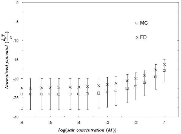
Electrostatic potential at one of the calcium binding sites for the epidermal growth factor-like calcium binding protein (PDB id: 1EDM). The electrostatic potential is computed for salt concentrations ranging from 0.000001M to 0.1M.
In the MCM, the electrostatic potential at any arbitrary site is calculated via a random walk starting from that precise 3D location, which implies that in order to compute the electrostatic potential at one particular location, one does not need to solve the LPBE over the entire 3-D computational domain as required in deterministic-based PBE approaches. Moreover, deterministic-PBE approaches do not provide site potentials directly- they only provide electrostatic potentials at the grid points and thus require the use of interpolation schemes in order to obtain potential values at any specified 3D-location. When we performed site electrostatic potential calculations for the epidermal growth factor protein using the Charmm force-field, we noted a large discrepancy (up to 20 %) between MCM and deterministic results which is due to the presence of internal voids that are caused by the small hydrogen atoms (radius = 0.2245 Å). It should be pointed out that if we considered the internal cavities as external regions in the deterministic computations as is done in the MCM solver, the agreement between the potential values obtained with both PBE algorithms would be restored. Moreover, we also noticed that the existence of internal cavities near one of the calcium binding sites, leads to extremely high electrostatic potentials, on the order of when such voids are treated as external regions.
In order to ensure small errors in the electrostatic potential calculations using the MCM simulations were performed with 1000 trajectories. The computations took at most 3 minutes to complete for any of the three calcium binding sites. We observed that the CPU time is smaller the further away the calcium site is from the molecular boundary. The CPU time can be further reduced by fine tuning code parameters such as the absorbing layer width, ε̄, and the auxiliary sphere radius, a. Our results suggest that the evaluation of electrostatic potential at putative recognition sites for large-scale biomolecular assemblies such as viruses and ribosomes using the proposed MCM will be of great interest to the structural biology and bioinformatics communities due its low cost and high accuracy.
4 Conclusions
We demonstrated the accuracy, memory and CPU time advantages of an alternative, stochastic-based, LPBE solver for obtaining salt-dependent electrostatic properties of biomolecules. In particular, we presented a detailed description of how correlated sampling is essential for obtaining accurate electrostatic properties of biomolecules over a broad range of salt concentration in a single MC-based PBE computation, thus significantly reducing the CPU cost and increasing the accuracy of the predictions of salt dependent electrostatic properties. We then validated the LPBE MCM by comparing the electrostatic potential and solvation free energies of calcium binding proteins against similar results obtained with a mature deterministic PBE solver. The excellent agreement between results obtained with two such fundamentally different techniques gives us confidence for further optimizing the present algorithm in order to make it a viable complementary LPBE solver for the general scientific community. We expect that our LPBE MCM will be very useful in predicting both the electrostatic potential at user-specified sites for large-scale biomolecular assemblies (e.g., viruses and ribosomes), and salt-dependent solvation free energies of proteins. The latter is important when examining the salt sensitivity of the stability of charged proteins.13 Of course, we anticipate that in the future it may be possible to create hybrid stochastic-deterministic PBE solvers, where we combine the strengths of each of these two fundamentally different numerical techniques.
Future work will include the applications of the LPBE MCM solver to the computation of other electrostatic properties (e.g., Born radii, electric field). In addition, there are many different quantities of biophysical interest (e.g., electrostatic binding free energy, pKa shift) that we wish to compute, and further algorithmic and code development is needed on the MCM. There are also many opportunities to improve the performance of MCM by using clever computational geometric algorithms. Finally, we anticipate that this approach will be increasingly beneficial to the general scientific community as these stochastic methods become both better developed and more widely deployed.
Acknowledgments
The authors thank Mr. Robert Harris and Dr. Alexander H. Boschitsch for stimulating discussion on different aspects of this work. MOF acknowledges support from 1R43GM079056-01 NIH-SBIR (PI: Dr. Alexander H. Boschitsch) and 5R01GM078538-03 NIH-NIGMS (PI: Dr.Michael Chapman, Co-PI: Dr.Marcia O. Fenley).
5 Appendix
5.1 Dependence of the Electrostatic Solvation Free Energy on κ
For the LPBE, the electrostatic free energy of a biomolecule immersed in a 1:1 salt solution is given as follows:89
| (11) |
where ρf is the charge density of the biomolecule, ϕ is the electrostatic potential, cb, is the bulk salt concentration, ε is the dielectric constant, and E⃗ is the electric field. From this equation one can derive two salt derivatives of the electrostatic free energy, namely and , where
| (12) |
In the equation (12), kb is the Boltzmann constant, T is the temperature, εe is the external dielectric constant, and e is the protonic charge.
The limiting behavior of these two salt derivatives of the electrostatic free energy at zero bulk salt concentration was first derived by Boschitsch et.al39,90 and are given as follows:
(i) The salt derivative of the electrostatic free energy w.r.t. κ:
From equation (11) one can derive the expression
| (13) |
where is the surface integral, ϕe is the electrostatic potential in the exterior region, and ue is the normalized potential .
At large distances from the biomolecule, the biomolecule can be treated effectively as a single central charge with total charge Qnet located in the center of a cavity of radius acav, which reflects the dimension of the biomolecule. In this region, the dielectric constant is εe, and the electrostatic potential, ϕe, has the following asymptotic form:
| (14) |
By using (14) and (12), as r → ∞, the limit of the derivative of ϕe w.r.t. κ at κ → 0 can be evaluated, and is given by . By using this, one can evaluate the surface integral S, in the limit of κ → 0, as follows:
| (15) |
The volume integral in equation (13) cannot generally be evaluated for arbitrary geometries. However the limiting behavior at κ → 0 can be computed exactly The exterior region can be divided into a region outside a spherical volume of radius Rs, called V2, and its complementary volume V1. Therefore the volume integral can be rewritten as:
| (16) |
The radius Rs is chosen to be large so that in region V2 the molecule looks like spherical object. Using the expression for the normalized electrostatic potential obtained from Kirkwood,91 the limit of I(V2) at κ → 0 can be calculated and is equal to for any finite Rs. Because I is independent of Rs, then it has to be true that the limκ→0I(V1) = 0. Therefore the limit of salt gradient at κ → 0 is given by:
| (17) |
as first shown by Boschitsch et.al.39,90
(ii) The salt derivative of the electrostatic free energy w.r.t. log(cb):
We begin by using the relationship
| (18) |
In the limit as κ → 0, the right terms of equation (18) are equal to zero, given the fact that the limiting behavior of S is defined by equation (15) and limiting behavior of volume integral I is given by . Therefore for any arbitrary geometry the following relation is valid:
| (19) |
(iii) The salt derivative of the electrostatic solvation free energy w.r.t. κ and log(cb):
Since is defined as
| (20) |
where the Gelec(εe = 1) is independent of κ, it is straightforward to calculate the limiting behavior of the two salt derivatives of as κ → 0 as
| (21) |
and
| (22) |
Footnotes
Supporting Information Available: This material is available free of charge via the Internet at http://pubs.acs.org.
References
- 1.Richard AJ, Liu CC, Klinger AL, Todd MJ, Mezzasalma TM, LiCata VJ. Biochim Biophys Acta. 2006;1764:1546–1552. doi: 10.1016/j.bbapap.2006.08.011. [DOI] [PubMed] [Google Scholar]
- 2.Niiranen L, Altermak B, Brandsal B, Leiros HK, Helland R, Smalas A, Willassen N. Febs J. 2008;275:1593–1605. doi: 10.1111/j.1742-4658.2008.06317.x. [DOI] [PubMed] [Google Scholar]
- 3.Kloss E, Barrick D. J Mol Biol. 2008;383:1195–1209. doi: 10.1016/j.jmb.2008.08.069. [DOI] [PMC free article] [PubMed] [Google Scholar]
- 4.Lindman S, Xue W, Szczepankiewicz O, Bauer MC, Nilsson H, Linse S. Biophys J. 2006;90:2911–2921. doi: 10.1529/biophysj.105.071050. [DOI] [PMC free article] [PubMed] [Google Scholar]
- 5.Suh JY, Tang C, Clore GM. J Am Chem Soc. 2007;129:12954–12955. doi: 10.1021/ja0760978. [DOI] [PubMed] [Google Scholar]
- 6.Henry BL, Connell J, Liang A, Krishnasamy C, Desai UR. J Biol Chem. 2009;284:20897–20908. doi: 10.1074/jbc.M109.013359. [DOI] [PMC free article] [PubMed] [Google Scholar]
- 7.Song B, Cho JH, Raleigh D. Biochemistry-US. 2007;46:14206–14214. doi: 10.1021/bi701645g. [DOI] [PubMed] [Google Scholar]
- 8.Majhi PR, Ganta RR, Vanam RP, Seyrek E, Giger K, Dubin PL. Langmuir. 2006;22:9150–9159. doi: 10.1021/la053528w. [DOI] [PubMed] [Google Scholar]
- 9.Müller-Santos M, de Souza EM, Pedrosa Fde O, Mitchell DA, Longhi S, Carrière F, Canaan S, Krieger N. Biochim Biophys Acta. 2009;1791:719–729. doi: 10.1016/j.bbalip.2009.03.006. [DOI] [PubMed] [Google Scholar]
- 10.Liu S, Low NH, Nickerson MT. J Agr Food Chem. 2009;57:1521–1526. doi: 10.1021/jf802643n. [DOI] [PubMed] [Google Scholar]
- 11.Watanabe EO, Popova E, Miranda EA, Maurer G, Pessôa Filho P de Alcântara. Fluid Phase Equilibr. 2009;281:32–39. [Google Scholar]
- 12.Yan W, Huang L. Int J Pharm. 2009;368:56–62. doi: 10.1016/j.ijpharm.2008.09.053. [DOI] [PMC free article] [PubMed] [Google Scholar]
- 13.Dominy BN, Perl D, Schmid FX, Brooks CL. J Mol Biol. 2002;319:541–554. doi: 10.1016/S0022-2836(02)00259-0. [DOI] [PubMed] [Google Scholar]
- 14.Bertonati C, Honig B, Alexov E. Biophys J. 2007;2:1891–1899. doi: 10.1529/biophysj.106.092122. [DOI] [PMC free article] [PubMed] [Google Scholar]
- 15.Formaneck MS, Ma L, Cui Q. J Am Chem Soc. 2006;128:9506–9517. doi: 10.1021/ja061620o. [DOI] [PMC free article] [PubMed] [Google Scholar]
- 16.Thomas AS, Elcock AH. J Am Chem Soc. 2006;128:7796–7806. doi: 10.1021/ja058637b. [DOI] [PubMed] [Google Scholar]
- 17.Ye X, Cai Q, Yang W, Luo R. Biophys J. 2009;97:554–562. doi: 10.1016/j.bpj.2009.05.012. [DOI] [PMC free article] [PubMed] [Google Scholar]
- 18.Min D, Li H, Li G, Berg BA, Fenley MO, Yang W. Chem Phys Lett. 2008;454:391–395. [Google Scholar]
- 19.Dzubiella J. J Am Chem Soc. 2008;130:14000–14007. doi: 10.1021/ja805562g. [DOI] [PubMed] [Google Scholar]
- 20.Feng J, Wong KY, Lynch GC, Gao X, Pettitt BM. J Phys Chem B. 2009;113:9472–9478. doi: 10.1021/jp902537f. [DOI] [PMC free article] [PubMed] [Google Scholar]
- 21.Li L, Liang S, Pilcher MM, Meroueh SO. Protein Eng Des Sel. 2009;22:575–586. doi: 10.1093/protein/gzp042. [DOI] [PubMed] [Google Scholar]
- 22.Massova I, Kollman PA. Perspect Drug Discov. 2000;18:113–115. [Google Scholar]
- 23.Fujiwara S, Amisaki T. Biophys J. 2008;94:95–103. doi: 10.1529/biophysj.107.111377. [DOI] [PMC free article] [PubMed] [Google Scholar]
- 24.Boda D, Valiskó M, Henderson D, Gillespie D, Eisenberg B, Gilson MK. Biophys J. 2009;96:1293–1306. doi: 10.1016/j.bpj.2008.10.059. [DOI] [PMC free article] [PubMed] [Google Scholar]
- 25.Lu B, Zhou Y, Holst M, McCammon JA. Commun Comput Phys. 2008;3:973–1009. doi: 10.4208/cicp.081009.130611a. [DOI] [PMC free article] [PubMed] [Google Scholar]
- 26.Grochowski P, Trylska J. Biopolymers. 2007;89:93–113. doi: 10.1002/bip.20877. [DOI] [PubMed] [Google Scholar]
- 27.Miertus S, Scrocco E, Tomasi J. Chem Phys. 1981;55:117–129. [Google Scholar]
- 28.Hoshi H, Sakurai M, Inoue Y, Chûjô R. J Chem Phys. 1987;87:1107–1115. [Google Scholar]
- 29.Zauhar R, Morgan R. J Comput Chem. 1988;9:171–187. [Google Scholar]
- 30.Rashin AA. J Phys Chem. 1990;94:1725–1733. [Google Scholar]
- 31.Yoon B, Lenhoff A. J Comput Chem. 1990;11:1080–1086. [Google Scholar]
- 32.Juffer A, Botta E, Vankeulen B, Vanderploeg A, Brendsen H. J Comput Phys. 1991;97:144–171. [Google Scholar]
- 33.Zhou HX. Biophys J. 1993;65:955–963. doi: 10.1016/S0006-3495(93)81094-4. [DOI] [PMC free article] [PubMed] [Google Scholar]
- 34.Bharadwaj R, Windemuth A, Sridharan S, Honig B, Nicholls A. J Comput Chem. 1995;16:898–913. [Google Scholar]
- 35.Purisima E, Nilar S. J Comput Chem. 1995;16:681–689. [Google Scholar]
- 36.Liang J, Subramaniam S. Biophys J. 1997;73:1830–1841. doi: 10.1016/S0006-3495(97)78213-4. [DOI] [PMC free article] [PubMed] [Google Scholar]
- 37.Vorobjev YN, Scheraga HA. J Comput Chem. 1997;18:569–583. [Google Scholar]
- 38.Totrov M, Abagyan R. Biopolymers. 2001;60:124–133. doi: 10.1002/1097-0282(2001)60:2<124::AID-BIP1008>3.0.CO;2-S. [DOI] [PubMed] [Google Scholar]
- 39.Boschitsch A, Fenley M, Zhou HX. J Phys Chem B. 2002;106:2741–2754. [Google Scholar]
- 40.Lu B, Cheng X, Huang J, McCammon JA. Proc Natl Acad Sci USA. 2006;103:19314–19319. doi: 10.1073/pnas.0605166103. [DOI] [PMC free article] [PubMed] [Google Scholar]
- 41.Hagstrom I, Fine R, Sharp K, Honig B. Proteins. 1986;1:47–59. doi: 10.1002/prot.340010109. [DOI] [PubMed] [Google Scholar]
- 42.Gilson M, Sharp K, Honig BH. J Comput Chem. 1988;9:327–335. [Google Scholar]
- 43.Davis M, McCammon J. J Comput Chem. 1989;10:386–391. [Google Scholar]
- 44.Nicholls A, Honig B. J Comput Chem. 1991;12:435–445. [Google Scholar]
- 45.Luty B, Davis M, McCammon J. J Comput Chem. 1992;13:1114–1118. [Google Scholar]
- 46.Holst M, Saied F. J Comput Chem. 1993;14:105–113. [Google Scholar]
- 47.Forsten K, Kozack R, Lauffenburger D, Subramaniam S. J Phys Chem. 1994;98:5580–5586. [Google Scholar]
- 48.Im W, Beglov D, Roux B. Comput Phys Commun. 1998;111:59–75. [Google Scholar]
- 49.Rocchia W, Alexov E, Honig B. J Phys Chem B. 2001;105:6507–6514. [Google Scholar]
- 50.Luo R, David L, Gilson M. J Comput Chem. 2002;23:1244–1253. doi: 10.1002/jcc.10120. [DOI] [PubMed] [Google Scholar]
- 51.Bashford D. Lect Notes Comput Sc. 1997;1343:233–240. [Google Scholar]
- 52.Cortis C, Friesner R. J Comput Chem. 1997;18:1591–1608. [Google Scholar]
- 53.Baker NA, Holst M, Wang F. J Comput Chem. 2000;21:1343–1352. [Google Scholar]
- 54.Holst M, Baker N, Wang F. J Comput Chem. 2000;21:1319–1342. [Google Scholar]
- 55.Shestakov A, Milovich J, Noy A. J Coll Interf Sci. 2002;247:62–79. doi: 10.1006/jcis.2001.8033. [DOI] [PubMed] [Google Scholar]
- 56.Chen L, Holst M, Xu J. Siam J Numer Anal. 2007;45:2298–2320. [Google Scholar]
- 57.Xie D, Zhou S. BIT. 2007;47:853–871. [Google Scholar]
- 58.Bhardwaj N, Stahelin RV, Langlois RE, Cho W, Lu H. J Mol Biol. 2006;359:486–495. doi: 10.1016/j.jmb.2006.03.039. [DOI] [PMC free article] [PubMed] [Google Scholar]
- 59.Freidlin M. Functional integration and partial differential equations. Princeton University Press; Princeton: 1985. pp. 117–163. [Google Scholar]
- 60.Tjong H, Zhou HX. J Chem Theory Comput. 2008;4:507–514. doi: 10.1021/ct700319x. [DOI] [PMC free article] [PubMed] [Google Scholar]
- 61.Geng W, Yu S, Wei G. J Chem Phys. 2007;127:114106. doi: 10.1063/1.2768064. [DOI] [PubMed] [Google Scholar]
- 62.Wang J, Cai Q, Li ZL, Zhao HK, Luo R. Chem Phys Lett. 2009;468:112–118. doi: 10.1016/j.cplett.2008.12.049. [DOI] [PMC free article] [PubMed] [Google Scholar]
- 63.Cai Q, Wang J, Zhao HK, Luo R. J Chem Phys. 2009;130:145101. doi: 10.1063/1.3099708. [DOI] [PubMed] [Google Scholar]
- 64.Zhou Z, Payne P, Vasquez M, Khn N, Levitt M. J Comput Chem. 1996;11:1344–1351. doi: 10.1002/(SICI)1096-987X(199608)17:11<1344::AID-JCC7>3.0.CO;2-M. [DOI] [PubMed] [Google Scholar]
- 65.Lu J, Deutsch C. J Mol Biol. 2008;384:73–86. doi: 10.1016/j.jmb.2008.08.089. [DOI] [PMC free article] [PubMed] [Google Scholar]
- 66.Lu J, Kobertz WR, Deutsch C. J Mol Biol. 2007;371:1378–1391. doi: 10.1016/j.jmb.2007.06.038. [DOI] [PubMed] [Google Scholar]
- 67.Gilson MK, Honig BH. Nature. 1987;330:84–86. doi: 10.1038/330084a0. [DOI] [PubMed] [Google Scholar]
- 68.Fleming C, Mascagni M, Simonov N. Lect Notes Comput Sc. 2005;3516:760–765. [Google Scholar]
- 69.Hwang CO, Mascagni M. Appl Phys Lett. 2001;78:787–789. [Google Scholar]
- 70.Karaivanova A, Mascagni M, Simonov N. Monte Carlo Methods Appl. 2004;10:311–320. [Google Scholar]
- 71.Mascagni M, Simonov N. SIAM J Sci Comp. 2004;26:339–357. [Google Scholar]
- 72.Simonov N. Dokl Math. 2006;74:656–659. [Google Scholar]
- 73.Simonov N. Lect Notes Comput Sc. 2007;4310:181–188. [Google Scholar]
- 74.Mascagni M, Simonov NA. J Comput Phys. 2004;195:465–473. [Google Scholar]
- 75.Simonov NA, Mascagni M, Fenley MO. J Chem Phys. 2007;127:185105. doi: 10.1063/1.2803189. [DOI] [PubMed] [Google Scholar]
- 76.Elepov B, Mikhailov G. Sov Math Dokl. 1973;14:1276–1280. [Google Scholar]
- 77.Ettelaie R. J Phys Chem. 1995;103:3657–3667. [Google Scholar]
- 78.Bondi A. J Phys Chem. 1964;68:441–451. [Google Scholar]
- 79.Dolinsky TJ, Nielsen JE, McCammon JA, Baker NA. Nucl Acids Res. 2004;32:665–667. doi: 10.1093/nar/gkh381. [DOI] [PMC free article] [PubMed] [Google Scholar]
- 80.Brooks BR, Bruccoleri RE, Olafson BD, States DJ, Swaminathan S, Karplus M. J Comput Chem. 1983;4:187–217. [Google Scholar]
- 81.Cornell WD, Cieplak P, Bayly CI, Gould IR, Merz KM, Ferguson DM, Spellmeyer DC, Fox T, Caldwell JW, Kollman PA. J Am Chem Soc. 1995;117:5179–5197. [Google Scholar]
- 82.Muller M. Ann Math Statistics. 1956;27:569–589. [Google Scholar]
- 83.Sabelfeld K. Monte Carlo methods in boundary value problems. Springer-Verlag; Berlin -Heidelberg - New York: 1991. [Google Scholar]
- 84.Bandyopadhyay AK, Sonawat HM. Biophys J. 2000;79:501–510. doi: 10.1016/S0006-3495(00)76312-0. [DOI] [PMC free article] [PubMed] [Google Scholar]
- 85.Lanyi JK. Microbiol Mol Biol Rev. 1974;38:272–290. [Google Scholar]
- 86.Baker NA, Sept D, Joseph S, Holst MJ, McCammon JA. P Natl Acad Sci USA. 2001;98:10037–10041. doi: 10.1073/pnas.181342398. [DOI] [PMC free article] [PubMed] [Google Scholar]
- 87.Penfold R, Warwicker J, Jönsson B. J Phys Chem B. 1998;102:8599–8610. [Google Scholar]
- 88.Jones S, Shanahan HP, Berman HM, Thornton JM. Nucl Acids Res. 2003;31:7189–7198. doi: 10.1093/nar/gkg922. [DOI] [PMC free article] [PubMed] [Google Scholar]
- 89.Sharp KA, Honig B. J Phys Chem. 1990;94:7684–7692. [Google Scholar]
- 90.Boschistsch AH, Fenley MO. J Comput Chem. 2004;25:935–955. doi: 10.1002/jcc.20000. [DOI] [PubMed] [Google Scholar]
- 91.Kirkwood JG. J Chem Phys. 1934;2:351–361. [Google Scholar]