Correlation between spatial-frequency and orientation-selectivity in V1 cortex: implications of a network model

Abstract

We addressed how spatial frequency and orientation selectivity coexist and co-vary in Macaque primary visual cortex (V1) by simulating cortical layer 4Cα of V1 with a large-scale network model and then comparing the model’s behavior with a population of cells we recorded in layer 4Cα. We compared the distributions of orientation and spatial frequency selectivity, as well as the correlation between the two, in the model with what we observed in the 4Cα population. We found that 1) in the model, both spatial frequency and orientation selectivity of neuronal firing are greater and more diverse than the LGN inputs to model neurons; 2) orientation and spatial frequency selectivity co-vary in the model in a way very similar to what we observed in layer 4Cα neurons; 3) in the model, orientation and spatial frequency selectivity co-vary because of intra-cortical inhibition. The results suggest that cortical inhibition provides a common mechanism for selectivity in multiple dimensions.

Introduction

Neuronal responses in primary visual cortex (V1) are selective in different spatial dimensions, such as orientation, spatial frequency, and size. Most theoretical work has focused on orientation selectivity, because it is the most well-studied functional property in V1. In most models (McLaughlin, Shapley, Shelley & Wielaard, 2000, Tao, Cai, McLaughlin, Shelley & Shapley, 2006, Tao, Shelley, McLaughlin & Shapley, 2004, Troyer, Krukowski, Priebe & Miller, 1998), neurons have diverse orientation selectivity but either no or fixed selectivity in other domains. In this paper, we study V1 neurons’ orientation selectivity and spatial frequency selectivity coexisting in a large-scale realistic model.

V1 neurons are much more sharply tuned to stimulus orientation and spatial frequency than are neurons in the Lateral Geniculate Nucleus (LGN). Orientation selectivity is generated in V1 (De Valois, Albrecht & Thorell, 1982, Hubel & Wiesel, 1962). V1 neurons inherit spatial frequency selectivity from LGN cells (So & Shapley, 1981), which in turn inherit it from retinal ganglion cells due to the center-surround organization of retinal receptive fields (Enroth-Cugell & Robson, 1966, Kuffler, 1953, Rodieck, 1965). However, the spatial frequency tuning of V1 neurons (Campbell, Cooper & Enroth-Cugell, 1969, De Valois et al., 1982, Movshon, Thompson & Tolhurst, 1978) is often much narrower than that of LGN cells. Traditional explanations of the increase in cortical spatial selectivity involve additive convergence of LGN input (Dayan & Abbott, 2001 for spatial frequency selectivity, De Valois & De Valois, 1988, Hubel & Wiesel, 1962 for orientation selectivity). However, intracellular data indicate that intra-cortical inhibition also could play a role in generating orientation selectivity (Anderson, Carandini & Ferster, 2000, Borg-Graham, Monier & Fregnac, 1998, Marino, Schummers, Lyon, Schwabe, Beck, Wiesing, Obermayer & Sur, 2005, Monier, Chavane, Baudot, Graham & Fregnac, 2003, Pei, Vidyasagar, Volgushev & Creutzfeldt, 1994, Schummers, Marino & Sur, 2002). Suppression of responses to non-preferred orientations (Malone & Ringach, 2008, Ringach, Bredfeldt, Shapley & Hawken, 2002a, Ringach, Shapley & Hawken, 2002b, Xing, Shapley, Hawken & Ringach, 2005) and non-preferred spatial frequencies (cf. Bredfeldt & Ringach, 2002, Ringach et al., 2002a) in reverse correlation experiments is additional evidence that inhibition may enhance selectivity.

The idea of a common mechanism, intra-cortical inhibition, for spatial selectivities seems plausible because there is a correlation between V1 neurons’ orientation and spatial frequency selectivity (De Valois et al., 1982, Xing, Ringach, Shapley & Hawken, 2004). De Valois et al. (1982) found a moderate correlation (r=0.5) between the bandwidths of V1 neurons’ orientation tuning and spatial frequency tuning. Xing et al. (2004) found a stronger correlation (r=0.78) between measures of spatial selectivity that compare responses at the peak of the tuning curve with responses to non-preferred stimuli: at non-optimal orientations, or at low spatial frequencies. The strong correlation between response attenuation of non-optimal stimuli in the two domains of orientation and spatial frequency led to the suggestion that there was a common mechanism: cortical response suppression (Xing et al., 2004).

This paper investigates a realistic model of V1 cortex and compares the model’s performance with cortical data. We found that 1) in the model, both spatial frequency and orientation selectivity of neuronal firing are greater and more diverse than the LGN inputs to model neurons; 2) orientation and spatial frequency selectivity co-vary in the model in a way very similar to what is observed in layer 4Cα; 3) in the model, orientation and spatial frequency selectivity co-vary because they both depend on intra-cortical inhibition. The results suggest that cortical inhibition provides a common mechanism for feature selectivity in multiple dimensions.

Methods

Large-scale network model

Complete details of the large-scale model we used can be found in Zhu et al. (2009). Our model resembled the models described in (McLaughlin et al., 2000, Tao et al., 2006, Tao et al., 2004, Wielaard, Shelley, McLaughlin & Shapley, 2001): a large-scale neuronal network of V1 layer 4Cα, consisting of 16,384 integrate-and-fire neurons, 75% of which are excitatory and 25% of which are inhibitory. It was a recurrent excitatory, inhibitory model with feedforward inputs from the LGN only. Each model neuron’s spike firing was governed by a standard integrate-and fire equation (equation 1) where the synaptic inputs to the neuron drove the membrane potential towards or away from the spike firing threshold.

$$\begin{array}{l}\frac{d{v}_{\sigma }^j}{dt}=-g_R(v_{\sigma }^j-V_R)-g_{\sigma E}^j(t)(v_{\sigma }^j-V_E)-g_{\sigma I}^j(t)(v_{\sigma }^j-V_I)\\ =-g_T^j(t)[v^j-V_S^j(t)],\end{array}$$ (1)

In eq. (1) the subscript σ = E, I denotes excitatory, inhibitory neurons respectively; for example v^j_E represents the membrane potential of an excitatory neuron at the location within the cortical layer indexed by j. When v^j_σ > V_Threshold, a spike was fired. Membrane capacitance was assumed to be a fixed constant, and was absorbed into the conductances so that g_R, g_E, g_I and g_T in equation 1 have the units sec⁻¹. In eq. (1), g_T = g_R + g_E + g_I is the total membrane conductance and V_S = (V_Eg_E + V_Ig_I)/g_T is the effective reversal potential. Voltage was normalized so that the resting potential V_R = 0 and V_Threshold = 1. Therefore, the reversal potentials of the excitatory and inhibitory synaptic currents, respectively V_E and V_I, were normalized to have the values 14/3 and 2/3. The leakage conductance g_R was set to 50 sec⁻¹.

The synaptic currents that appear in eq (1) were set by the pattern of LGN and intra-cortical connectivity built into the model through expressions for the synaptic conductances (equation 2).

$$\begin{array}{l}{g}_{EE}^j(t)=g_{\mathit{lgn}}^j(t)+g_{\mathit{noise}}^j(t)+S_{EE}^j\sum _k{a}_{j-k}{p}_{j-k}\sum _m{G}_E(t-t_m^k),\\ g_{EI}^j(t)=S_{EI}^j\sum _k{b}_{j-k}\sum _m{G}_I(t-t_m^k),\\ g_{IE}^j(t)=g_{\mathit{lgn}}^j(t)+g_{\mathit{noise}}^j(t)+S_{IE}^j\sum _k{a}_{j-k}{p}_{j-k}\sum _m{G}_E(t-t_m^k),\\ g_{II}^j(t)=S_{II}^j\sum _k{b}_{j-k}\sum _m{G}_I(t-t_m^k).\end{array}$$ (2)

The spatial coupling coefficients a_j−k and b_j−k in eq. (2) were approximated by Gaussian functions of cortical distance between cells j and k. The Gaussian length scales for excitation and inhibition were 200μm and 100μm, respectively, derived from neuroanatomical measurements as in McLaughlin et al (2000). The term g_noise in eq. (2) was a constant noise source presumed to come from cortico-cortical inputs that are not visually driven, and was needed to explain the higher spontaneous firing rates of complex cortical cells that receive only weak or no LGN excitatory drive (Zhu et al., 2009).

The spatial pattern of intra-cortical connectivity in the model was local, via intra-hypercolumn connections, based on neuroanatomical measurements of V1 circuitry (Callaway, 1998, Fitzpatrick, Lund & Blasdel, 1985). Each model neuron received hundreds of synaptic inputs, both excitatory and inhibitory, through random connections from its neighbors with no spatial phase preference and with an orientation preference given by the map of orientation onto the cortex (McLaughlin et al., 2000, Tao et al., 2004).

In the model, the spatial pattern of LGN input to a single model neuron was side-by-side elongated sub-regions. We put spatial frequency information into the construction of those elongated regions by allowing different sub-region widths (Zhu et al., 2009). There are optical imaging data (Sirovich & Uglesich, 2004) and single unit data (DeAngelis, Ghose, Ohzawa & Freeman, 1999) from V1 that suggest that nearby cells have similar spatial frequency preferences but that beyond a fairly short distance the cells’ preferences are unrelated. To be consistent with these data, we divided the network into many clusters of cells, inside each of which the V1 neurons share the same width of their LGN input arrays. Clusters of different width were arranged randomly across the V1 layer. Moreover, the spatial pattern of LGN inputs to each V1 neuron was set randomly to have even or odd symmetry, i.e, for an even symmetric neuron, the LGN input to the elongated sub-regions could be of the form ON-OFF-ON or OFF-ON-OFF. Such a random assignment of symmetry is also compatible with cortical data (DeAngelis et al., 1999, Ringach, 2002). The choice of the pattern of LGN input was strictly determined by experimental data, as explained more fully in Zhu et al (2009), following the approach of incorporating biological data in the modeling that was used by McLaughlin et al (2000). The LGN cell firing rates were modeled as inhomogeneous Poisson processes where the rate parameter of each Poisson process was modulated by a spatio-temporally filtered version of the visual input (cf. Tao et al., 2004, Zhu et al., 2009).

The cortico-cortical conductance coupling matrix was a crucial part of the model. The coupling coefficients were chosen to obtain a model that responded to visual stimuli as V1 cortex did, both in terms of selectivity but also in terms of firing rates. The values in the conductance coupling matrix in equation (2) were: recurrent excitation’s coefficient S_EE = 0.1 sec⁻¹ at its minimum (for cells that receive maximal LGN input), and S_EE=45 sec⁻¹ for its maximum value (for cells that receive no LGN input); the coupling strength for inhibitory synapses onto excitatory neurons S_EI=80 sec⁻¹; the strength of cortical excitation of inhibitory neurons, S_IE = 0.1–46 sec⁻¹ for the range between its minimum and maximum values; inhibition’s strength on inhibitory neurons, S_II = 65sec⁻¹. These coupling coefficients represent the amount of synaptic conductance increase per nerve impulse from the source neurons. With this conductance matrix, the cortical model was in a high conductance state (Shelley, McLaughlin, Shapley & Wielaard, 2002), considered in the Discussion.

Animal experiments

Preparation

Acute experiments of several days duration were performed on adult old-world monkeys (M. fascicularis) in compliance with National Institutes of Health (NIH) and New York University (NYU) guidelines, with the approval of the New York University Animal Welfare Committee. Procedures were like those described in detail in Xing et al (2004). Animals were initially tranquilized with acepromazine (50 μg/kg). After the tranquilizer, the animal was anesthetized by ketamine (30 mg/kg, intramuscularly, im) for venous cannulation and tracheotomy. Additional ketamine was given during this surgery if needed. After cannulation and tracheotomy, the animal was placed in a stereotaxic frame for craniotomy and subsequent visual experiments. Further surgery was performed under sufentanyl (6–18 μg/kg/h, intravenously, iv) anesthesia (infused through a leg vein, usually the left-leg vein). A craniotomy (5mm or smaller in radius) was made in one hemisphere 4mm posterior to the lunate sulcus (15–20mm anterior to the occipital ridge) and 15mm lateral to the middle line. Then the dura was cut (less than 1mm in radius) to provide access for the electrode. Triple antibiotic ointment was applied surrounding the incision. During the whole acute experiment, anesthesia was continued with sufentanyl (6–18 μg/kg/h, iv) and the animal was paralyzed with vecuronium bromide (0.1 mg/kg/h, iv) (infused through a venous cannula on another leg). After the animal was paralyzed, respiration was supported by a respirator (Harvard Apparatus) to maintain expired CO₂ close to 5%. Temperature was kept at a constant 37°C. A broad- spectrum antibiotic (Bicillin, 50,000 iu/kg, im) and anti-inflammatory steroid (dexamethasone, 0.5 mg/kg, im) were given on the first day of the experiment and every other day during the recording period. Experiments were terminated with a lethal dose of pentobarbital (60 mg/kg, iv). Expired CO₂, blood pressure, EKG, EEG and core body temperature were monitored continuously, and were used to make sure that anesthesia was maintained at a steady level. Ophthalmic atropine sulfate (1%) was administered to the eyes at the start of the experiment in order to dilate the pupils. Throughout the experiment, the eyes were protected by clear, gas-permeable contact lenses and a topical antibiotic solution (gentamicin sulfate, 3%). The foveae were mapped onto a tangent screen using a reversing ophthalmoscope. Glass-coated tungsten microelectrodes were advanced through a craniotomy over occipital cortex. Cells were recorded in V1, typically in the region that represents 2–6 degrees eccentricity. Extracellular spikes were discriminated and time-stamped with 0.1 ms resolution via custom software running on a Silicon Graphics O2. The visual receptive fields of isolated single neurons were mapped onto the tangent screen with reference to the foveae. Using histological techniques we assigned cells to layer 4Cα. This paper is the first study that includes this population of 4Cα neurons.

Histology

We compared orientation and spatial frequency selectivity of the model population with cell data from layer 4Cα. Cells were assigned to layer 4Cα by track reconstruction following procedures described by Hawken et al (1988). Briefly, three to six electrolytic lesions (2–3 μA for 2–3 sec, tip negative) were made along the length of each electrode track. The angle of the electrode track, relative to the surface normal, was approximately 60deg. A typical electrode track would extend for about 3–4mm. Consecutive lesions were spaced by about 1mm. Our electrode tracks resembled the one shown in Hawken and Parker (1984). The details of fixation, sectioning, staining and reconstruction of electrode tracks are described by Hawken et al. (Hawken et al., 1988).

Visual stimulation

Each isolated single-cell was stimulated monocularly through its dominant eye and characterized by measuring its steady-state response to conventional drifting gratings (the non-dominant eye was occluded). Using this method we recorded basic attributes of the cell, including spatial and temporal frequency tuning, orientation tuning, contrast and color sensitivity, as well as area summation curves. Receptive fields were located at eccentricities between 1 and 6 deg. The mean luminance of the screen was 50 cd/m², the viewing distance 90–120 cm.

Spatial Frequency and Orientation Tuning Curves

In the present experiments, we measured tuning curves for steady state stimuli, drifting gratings, which vary in orientation and spatial frequency. We have described in detail the procedures for measuring the orientation tuning to drifting grating stimuli and the analysis of the tuning curves (Ringach et al., 2002b). Briefly, orientation was measured in steps of 20 degrees or less, for stimuli of the optimal spatial and temporal frequency. In the standard experiments contrast was usually 0.8 (though occasionally it was set arbitrarily to 0.64, with no obvious difference in tuning curves). Spatial frequency tuning was determined in half octave steps for a range of frequencies that covered the response range of each cell. For each cell, the size of the circular stimulus window was chosen to optimize response. Each tuning function was fit with a difference of Gaussians to obtain a smooth curve for calculating the spatial frequency bandwidth (Sceniak, Hawken & Shapley, 2001).

Data Analysis

Orientation tuning bandwidth

Given a cell’s orientation tuning curve, we smoothed the curve with a Hanning window filter of width 18°. Then we found the peak response in the smoothed curve, and looked for the points on both sides of the peak at which the cell’s responses were half of the peak response. Half of the distance between the two points is the orientation bandwidth.

$${\mathit{Ori}}_{\text{bw}}=[{\mathit{Ori}}_{1/2,\text{high}}-{\mathit{Ori}}_{1/2,\text{low}}]/2$$ (3)

If there was no response smaller than half of the peak, then the cell was called non-oriented and its orientation tuning bandwidth set to 180°.

Circular variance (CV)

To determine a cell’s orientation tuning curve we measured 18 different responses of the cell to orientations over the range 0 and 360⁰ with 20⁰ intervals. We denote the spike rate responses m(θ_i) (i=1,2, …18) for each orientation. Circular variance for a tuning function m(θ) on a circle is defined by the following equation (Mardia, 1972)

$$CV[m]=1-\frac{\mid {\int }_0^{2\pi }m(\theta )exp(2i\theta )d\theta \mid }{{\int }_0^{2\pi }m(\theta )d\theta }$$ (4)

Circular variance is highly correlated with other measures of orientation selectivity like the ratio of orthogonal-to-preferred response divided by preferred response (Ringach et al., 2002b). CV lies between 0 and 1. Highly selective cells have a CV ~0, while unselective cells have CV=1.

In the spatial frequency-tuning experiments, we used drifting gratings with optimal orientation, temporal frequency, radius, and high contrast to stimulate the cell’s receptive field. Cells’ responses were measured to ten gratings of different spatial frequencies evenly distributed between 0.1 and 10 c/deg on a logarithmic scale. Then we fit the data with a DOG (difference of Gaussians) model as in equation 5, by minimizing the square error between the DOG curve and the data, with all parameters (R₀, K_e, μ_e, σ_e, K_i, μ_i, and σ_i) free.

$$R(SF)=R_0+K_{e}exp(-\frac{{(SF-{\mu }_e)}^2}{2{\sigma }_e^2})-K_{i}exp(-\frac{{(SF-{\mu }_i)}^2}{2{\sigma }_i^2})$$ (5)

Spatial frequency tuning bandwidth

We found the peak of the fitted spatial frequency tuning curve, and looked for the points where the curve dropped to half of the peak, denoted Sf_high and Sf_low. The spatial frequency bandwidth (in octaves) is defined in the following equation.

$${Sf}_{bw}=lo{g}_2({Sf}_{\mathit{high}})-lo{g}_2({Sf}_{\mathit{low}})$$ (6)

If the cell’s response at the lowest spatial frequency measured (0.1 cycle/deg) was higher than half the best response, we defined the cell as low-pass, without a bandwidth. In layer 4Cα, about 90% of simple cells (28/30) had a measurable bandwidth in both spatial frequency and orientation.

Low spatial frequency variance (LSFV)

Based on the fitted spatial frequency tuning curve, the left branch of the curve from 1/M (we usually chose M=16 points) of the optimal spatial frequency to the optimal spatial frequency was used to calculate Low Spatial Frequency Variance (LSFV; introduced in Xing et al (2004)) by means of equation 7.

$$\mathit{LSFV}=\frac{\underset{{Sf}_{\mathit{optimal}}/16}{\overset{{Sf}_{\mathit{optimal}}}{\int }}R(Sf)\times {(lo{g}_{16}(Sf)-lo{g}_{16}({Sf}_{\mathit{optimal}}))}^2\times {\mathit{dlog}}_{16}(Sf)}{\underset{{Sf}_{\mathit{optimal}}/16}{\overset{{Sf}_{\mathit{optimal}}}{\int }}R(Sf)\times {\mathit{dlog}}_{16}(Sf)}$$ (7)

LSFV is a global measure that assesses the degree of low spatial frequency attenuation. It captures the global shape of a spatial-frequency tuning curve while the bandwidth characterizes the shape of the tuning curve near the peak (preferred) spatial frequency. The LSFV measure is smaller when the cell is more selective for spatial frequency. LSFV has a value of 0 for the most spatial-frequency-selective cells; for a low-pass (unselective) neuron, LSFV = 1/3 (Xing et al., 2004).

Results

In this study, we simulated a 1mm X 1mm patch of cortical layer 4Cα of V1 with a large-scale network model consisting of O(10⁴) excitatory and inhibitory integrate-and-fire neurons with realistic synaptic conductances (Zhu et al., 2009). Some features of our model were similar to other cortical network models (Chance, Nelson & Abbott, 1999, McLaughlin et al., 2000, Tao et al., 2006, Tao et al., 2004, Troyer et al., 1998), but this new model allowed us to study model V1 neuronal responses in both orientation and spatial frequency domains. The model successfully simulated several functional properties similar to those in the real 4Cα data that we present for comparison, including: 1) functionally distinct simple and complex cells; 2) diversity of orientation and spatial frequency selectivity similar to experimental results; 3) correlation between the orientation and spatial frequency selectivity.

In this work, the visual stimuli considered were drifting gratings. We tested the large-scale model under 64 experimental conditions, by applying stimuli with 8 orientations (0, 45, 90, 135, 180, 225, 270, 315 deg) and 8 spatial frequencies (1/16, 1/8, ¼, ½, 1, 2, 4, 8 cycle/deg) and with the highest contrast (100%). For each model neuron, the preferred orientation and preferred spatial frequency were taken to be those values where the spike rate was highest among the 64 simulated experiments.

Simple and complex cells

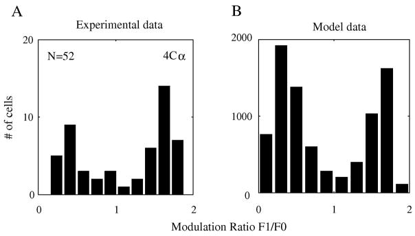
Although it is not the main result of our current paper, we need to point out that our large-scale model generated simple and complex cells with a distribution like that seen in the biological cortex (Figure 1). We show this result at the beginning, because the following results are mainly focused on simple cells’ behavior in the network. A traditional way to differentiate simple cells from complex cells with respect to drifting grating patterns is by means of the modulation ratio F1/F0 (Skottun, De Valois, Grosof, Movshon, Albrecht & Bonds, 1991): cells with F1/F0>1 are called simple while cells F1/F0<1 are called complex, where F1 and F0 are the first harmonic amplitude and one half of the mean firing rate, respectively. Experimentally we found a bimodal distribution of F1/F0 in layer 4Cα (Figure 1A) that is similar to the distribution of modulation ratio observed throughout V1 (Ringach et al., 2002b, Xing et al., 2004). The large-scale model generated a bimodal distribution that was similar to experimental data (Figure 1B). The bimodal distribution of F1/F0 in the V1 model was in part a consequence of the nonlinearity of spike threshold as hypothesized by Mechler & Ringach (2002) and Priebe et al. (2004). The distribution of F1/F0 in the model neurons’ membrane potentials was unimodal (cf. Tao et al., 2004). It is useful to examine the feature selectivity of simple and complex cells separately because there was a strong correlation of feature selectivity with F1/F0 ratio in the model as in the real cortex (Ringach et al., 2002b, Xing et al., 2004) as we will show.

Figure 1. Segregation of Simple and Complex cells in the model v.s experimental data.

A: Modulation ratio F1/F0 of individual neurons from Layer 4Cα in V1 has a bi-modal distribution. B: In our large-scale network model, the distribution of F1/F0 is very similar to that for experimental data in A.

Diversity of orientation selectivity and spatial frequency selectivity: examples

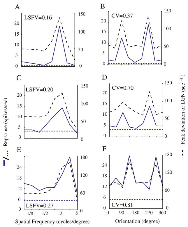
The tuning curves for selected example simple cells in the model illustrate how the model achieves selectivity for spatial frequency and orientation (Figure 2). The spatial frequency tuning (solid curves in Fig. 2A, C and E) and orientation tuning (solid curves in Fig 2B, D and F) of the spike rates of simple cells in the model network resembled experimental results in V1 (Ringach et al., 2002b, Xing et al., 2004). In order to understand the mechanism of spatial frequency and orientation selectivity, we plotted in the same graphs the orientation and spatial frequency tuning curves of excitatory synaptic current from the summed LGN inputs to the model simple cells (dashed curves in Fig. 2). The difference between model neurons’ tuning curves and those of their LGN inputs can be seen mainly in the attenuation of the spike-firing rate to non-optimal stimuli. In general, the LGN inputs from cell to cell had similar, rather low, selectivity because the LGN inputs in Fig. 2 had much higher responses to non-optimal orientations relative to their peak responses, and relatively higher responses to low spatial frequencies than the model V1 neurons.

Figure 2. Simple cells’ Orientation and spatial frequency tuning curves in the model neurons.

Spatial frequency tuning curves (solid blue curves in A, C and E) were plotted for 3 example cells from the network. Corresponding orientation tuning curves were also plotted (solid curves in B, D and F). Dashed curves in A-F represent the orientation or spatial frequency tunings of the 3 cells’ LGN inputs. The dashed horizontal lines indicate the background spike rate, the firing rate when there was no stimulus contrast. The spatial frequency LSFV and orientation CV for the three examples were respectively: (0.16, 0.37), (0.2, 0.7), (0.27, 0.81). In A, C, E the LSFVs of the LGN inputs were 0.26, 0.27 and 0.26; in B, D, F the CVs were 0.73, 0.87 and 0.84.

To summarize the tuning properties of neurons, one needs a measure of selectivity for each tuning curve. It has been shown that circular variance (CV) for orientation tuning and low spatial frequency variance (LSFV) for spatial frequency tuning are measures of feature selectivity that indicate the degree of attenuation of responses to non-optimal stimuli, as well as the global selectivity in these two domains (see Methods; Ringach et al., 2002a, Xing et al., 2004). It has been shown previously CV is highly correlated with other measures of orientation selectivity like the orthogonal/preferred ratio (Ringach et al., 2002b), and that LSFV is a measure of the shape of the spatial frequency tuning curve that correlates with other measures like Low-Spatial-Frequency-Selectivity Index (Xing et al., 2004). The relatively weak selectivity of the LGN inputs can be quantified by the LSFV and CV of the LGN inputs. In A, C, E the LSFVs of the LGN inputs were 0.26, 0.27 and 0.26; in B, D, F the CVs were 0.73, 0.87 and 0.84. Fig. 2 indicates that cell spike-firing at non-optimal orientations and lower spatial frequencies was suppressed in the cortex for the most selective cells. Thus, the LSFV’s for the spike firing rates in examples A, C, E were 0.16, 0.2, and 0.27 and the CVs in B, D, and F were 0.37, 0.7, and 0.81 respectively. The firing rates of more selective cells as in Fig. 2AB had lower LSFV and CV than their LGN inputs.

The examples in Fig. 2 were representative of the whole population, as we will show. But different cortical cells varied in selectivity as Fig. 2 also illustrates. The variation was mainly in how weak were the non-preferred responses compared to preferred responses. As Fig 2 also illustrates, when spatial frequency selectivity was high, so also was orientation selectivity (Fig 2AB), and when the selectivity for spatial frequency was less, also the orientation selectivity was less (Fig. 2EF). The correlation seen in the examples of Fig. 2 also applied to the entire V1 model population, as shown below in Figure 6.

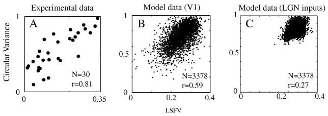
Figure 6. Correlation between orientation selectivity and spatial frequency selectivity (Simple cells).

The network model generates a correlation pattern (B) for simple cells’ orientation and spatial frequency selectivity. This pattern resembles the pattern from experimental data (A) for simple cells in layer 4Cα in V1. But the correlation pattern (B) for simple cells is very different from the correlation pattern for simple cells’ summed LGN synaptic input currents in (C). The strengths of correlation are indicated by the correlation coefficients written within each figure panel.

Diversity of orientation selectivity and spatial frequency selectivity: population analysis

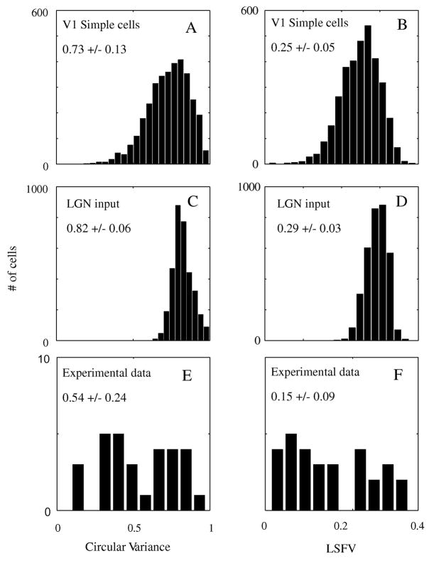
For a population analysis of orientation and spatial frequency selectivity we plotted the distributions of CV and LSFV for the population of model simple cells and their LGN inputs (Figure 3). The shifts of the population distributions to the left for the firing rates compared to LGN inputs, for both CV and LSFV, mean that the firing rates of model simple cells (Fig 3A and B) were more selective on average than their LGN inputs (Fig 3C and D) in the dimensions of orientation and spatial frequency. Also, the model V1 cells had a wider range of selectivity than their LGN inputs--the distributions for cell firing rates were broader than for the LGN inputs. The diversity of selectivity in the model network resembled the diversity seen in the real cortex in layer 4Cα (Fig 3E, F) but the 4Cα population sampled in the experiments had a wider range of diversity of spatial frequency and orientation selectivity than the model population.

Figure 3. Distribution of CV and LSFV for V1 simple cells vs the distribution of CV and LSFV for their LGN inputs (Simple cells).

The orientation selectivity and spatial frequency selectivity of the population of model simple cells (A and B) were greater than those of their LGN inputs (C and D). The LGN inputs were the summed excitatory synaptic currents coming from LGN inputs. The range of selectivity for V1 simple cells is also wider than that for simple cells’ LGN inputs; the distributions in A and B are broader than in C and D. The distributions of orientation selectivity and spatial frequency selectivity for the dataset of 4Cα neurons from the real cortex are plotted in E and F respectively.

The model’s diversity is generated by interactions within the cortical network. It is evident in the simple cell examples from the model in Fig. 2 that, for selective neurons, LGN excitation at non-preferred orientations and spatial frequencies had a reduced influence on the model cells’ spike rates. In the orientation domain this suppression was caused by broadly-tuned inhibition in the model (Cf. McLaughlin et al., 2000). In the spatial frequency domain, suppression of low-spatial frequency responses was caused by intra-cortical inhibition that was stronger than excitation at low spatial frequency, as analyzed in detail by (Zhu et al., 2009). The combination of broadly tuned inhibition and the spike-firing threshold of V1 neurons caused the spike rates of many simple cells in the model to be much more selective for spatial frequency and orientation than their LGN inputs were.

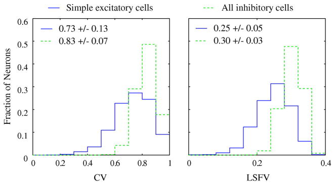
Individual inhibitory neurons in the model were considerably less selective than model simple excitatory cells (Figure 4) as indicated by the higher CV of inhibitory neurons for orientation selectivity (Fig 4A) and as indicated by their higher LSFV for spatial frequency selectivity (Fig 4B). The different tuning characteristics of inhibitory neurons in the model was in part a consequence of their higher spontaneous firing rates and also their higher firing rates in response to visual stimulation (McLaughlin et al., 2000, Zhu et al., 2009), as well as to their denser intra-cortical connectivity. The existence of inhibitory neurons in visual cortex that were broadly-tuned (or untuned) for orientation was reported recently (Cardin, Palmer & Contreras, 2007, Nowak, Sanchez-Vives & McCormick, 2008), consistent with model results. We also observed relatively higher spike rate responses of model inhibitory neurons for lower spatial frequencies (cf. Fig. 12 of Zhu et al., (2009)), consistent with experimental data (Cardin et al., 2007, Nowak et al., 2008).

Figure 4. Distribution of CV and LSFV for excitatory and inhibitory cells in the model.

Dashed contours show the distribution of inhibitory neurons’ circular variance (A: mean 0.83+/−0.05) and LSFV (B: mean 0.30+/−0.028). Solid contours show the distribution of excitatory simple cells’ circular variance or CV (A: mean 0.73+/−0.13) and LSFV (B: 0.25+/−0.05).

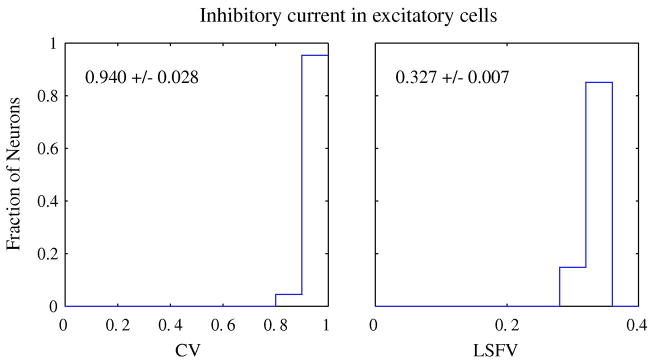
The convergence of many inhibitory neurons onto excitatory neurons was what made the orientation and spatial frequency tuning of intracellular inhibition in model neurons almost constant with orientation and strong at low spatial frequency (Zhu et al., 2009). The tuning characteristics of the summed inhibitory current on excitatory cells were very broad--almost flat with orientation and low-pass in spatial frequency as quantified by the distributions of inhibition’s LSFV and CV across the V1 population in Figure 5. We conjecture that such broadly-tuned inhibition from the local hypercolumn circuit is probably what causes the Untuned Suppression observed in reverse correlation experiments (Xing et al., 2005), and also probably is the source of low-spatial-frequency suppression that is observed in reverse correlation experiments (Bredfeldt & Ringach, 2002, Ringach et al., 2002a).

Figure 5. Distribution of CV and LSFV for the inhibitory current in excitatory cells.

The CV and LSFV were calculated for the inhibitory currents in excitatory neurons in the model. The uniformly high values of CV and LSFV indicate that inhibitory current in model neurons was untuned for orientation and low-pass in spatial frequency. The mean CV for the inhibitory current was 0.94+/−.028. The mean LSFV was 0.327+/−0.007.

Correlation between orientation selectivity and spatial frequency selectivity

The presence of diversity in selectivity as illustrated in Fig. 3 enabled us to study correlations between orientation and spatial frequency selectivity in the real cortex and in the model. This is the crucial comparison in this paper. The distributions of orientation and spatial frequency selectivity in the model (Fig 3) resembled experimental data. The correlation between simple cells’ spatial frequency and orientation selectivity in the model network (illustrated with the scatter plots in Figure 6) also was similar to experimental results (cf. De Valois et al., 1982, Xing et al., 2004).

As reported previously (Xing et al., 2004), LSFV was strongly correlated with CV in experimental data from all of V1 cortex. Experimental data from cells in layer 4Cα also had a strong correlation between CV and LSFV (Fig. 6A for cells in layer 4Cα; cf. Xing et al., 2004 for all cortical cells in V1); the correlation for layer 4Cα simple cells was 0.81. Figure 6B indicates that in the model also, orientation selectivity measured by circular variance, CV, was highly correlated with spatial frequency selectivity measured by low-spatial-frequency-variance, LSFV, with a correlation coefficient of 0.59. We found that the strong correlation between CV and LSFV in the large-scale network model was not due to simple cells’ LGN inputs (the summed excitatory current from LGN synaptic inputs onto model neurons), which had a much weaker correlation between orientation and spatial frequency selectivity, only 0.27 (Fig. 6C). Therefore, a cortical mechanism was required to explain the correlation between orientation and spatial frequency selectivity.

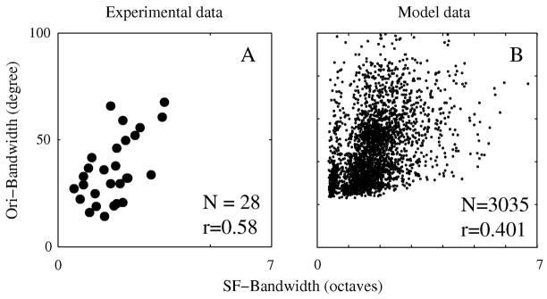
The correlation between orientation and spatial frequency bandwidth throughout V1 was noted by DeValois et al (1982) and replicated by Xing et al (2004). As in the whole of V1, the bandwidth correlation was weaker than between CV and LSFV in layer 4Cα simple cells (Figure 7A). The large-scale model emulated layer 4Cα in this respect too (Figure 7B).

Figure 7. Correlation between orientation bandwidth and spatial frequency bandwidth (Simple cells).

The network model generates a correlation pattern (B) for orientation and spatial frequency bandwidth similar to the pattern in real 4Cα data (A).

Our explanation for the resemblance of the correlations in model and real cortex is the hypothesis that a single mechanism, which we suppose is the suppression caused by cortical inhibition, plays a similar role in orientation selectivity and spatial frequency selectivity (cf. Ringach et al., 2002a). In the model, local cortical inhibition acts like shunting inhibition (cf. Shelley et al., 2002), a point we take up in the Discussion. Next we explore this inhibition hypothesis by examining the link between variations in inhibitory conductance and selectivity in the V1 model.

Synaptic conductance and orientation and spatial selectivity

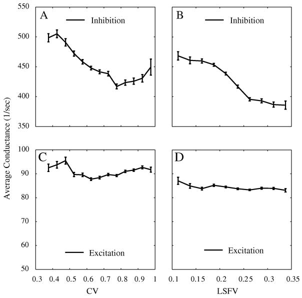
The model emulated the behavior of V1 in having a strong correlation between orientation and spatial frequency selectivities, as shown in Fig. 6. This suggests that we could understand the relation between these selectivities in V1 by trying to understand their relation in the model. The way we did this was by plotting spatial frequency LSFV and orientation CV versus the inhibitory and excitatory conductance strength for the population of model neurons. The conductance strength for each model cell was quantified as the average synaptic conductance during visual stimulation, averaged across all stimuli in one dimension, for instance averaged across all eight spatial frequencies used as stimuli to obtain the model cell’s spatial frequency tuning curve. Figure 8A and C show the relation between strengths of inhibitory and excitatory synaptic conductances and the orientation CV for simple cells (Zhu et al., 2009). Higher amounts of average synaptic inhibition were associated with lower CV (more orientation selectivity). There appeared to be no consistent relation between variation in excitatory synaptic conductance and CV for model simple cells. Figure 8B and D show the relation between strengths of inhibitory and excitatory synaptic conductances and spatial frequency LSFV for simple cells. Higher amounts of selectivity, lower LSFV, were associated with stronger mean inhibition. Synaptic conductance strengths in the model varied because of location within the layer of V1, because of variations in the total amount of cortical input from neighboring neurons. What Figure 8 indicates is that the variation of inhibitory synaptic strength across the population was an underlying variable that caused the observed correlation between orientation and spatial frequency selectivity.

Figure 8. Inhibition, excitation and selectivity for simple cells.

Plots of mean inhibition and excitation vs circular variance and LSFV. Standard errors indicated by the error bars. There is a correlation between simple cells’ selectivity and the inhibition they received in both orientation (A) and spatial frequency (B) domain. However, there is no such relationship between simple cells’ selectivity and their excitation (C and D). The mean excitation and inhibition value for each model neuron is the average over time and over the responses to the eight stimuli used to obtain a tuning curve in each domain.

Another way to analyze the influence of cortical mechanisms on the correlation of selectivities is to seek differential patterns of amount of synaptic input in the scatter plots of orientation vs spatial frequency selectivity. To do this we re-plotted the scatter plot originally shown in Fig. 6B but used only a randomly selected sub-sample of 10 % of the cells in the model so that individual points could be visualized. We marked each point (each model simple cell) with a color that signified the average amount of inhibition (Figure 9) or excitation (Figure 10). Fig. 9 shows that the model simple cells that had higher selectivities for both orientation and spatial frequency tended to have higher average inhibitory input. Model simple cells that had lower average inhibitory input tended to be located in the scatter plot in the region of low selectivity. There was no consistent pattern for excitation (Fig. 10). These cell-by-cell analyses support the conclusions based on population averages in Fig. 8.

Figure 9. Correlation between orientation and spatial frequency selectivity and inhibition.

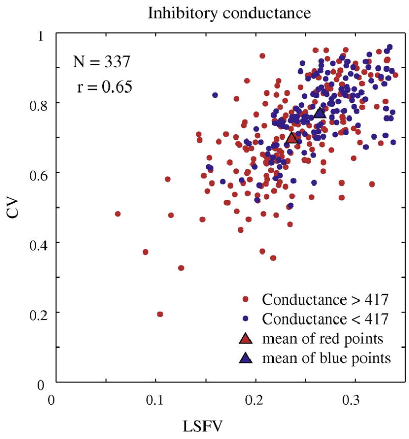
The correlation pattern of orientation and spatial frequency selectivity for a randomly selected subset (N=337) of model simple cells. Each cell is marked by a color that indicates its average inhibitory conductance across the fifteen experimental runs that were used to generate the orientation and spatial frequency tuning curves. The cells with higher average conductances tend to plot to the lower left hand region of the cloud of points while the cells with lower average inhibitory conductance tend to plot to the upper right hand region of the plot, the region of low selectivity in both domains.

Figure 10. Correlation between orientation and spatial frequency selectivity and excitation.

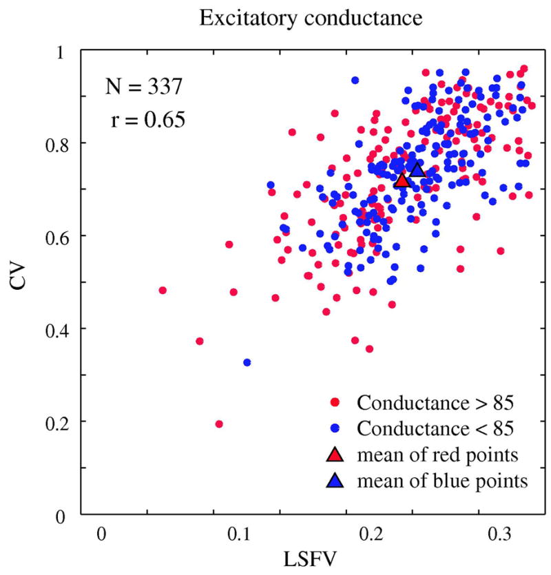
The correlation pattern of orientation and spatial frequency selectivity for a randomly selected subset (N=337) of model simple cells. Each cell is marked by a color that indicates its average excitatory conductance across the 15 experimental runs that were used to generate the two tuning curves for orientation and spatial frequency. There is no clear pattern of clustering of cells with low or high average excitatory conductance.

Another way to illustrate this important point is to divide the cell population along the regression line of correlation between orientation and spatial frequency selectivity, as in Figure 11.

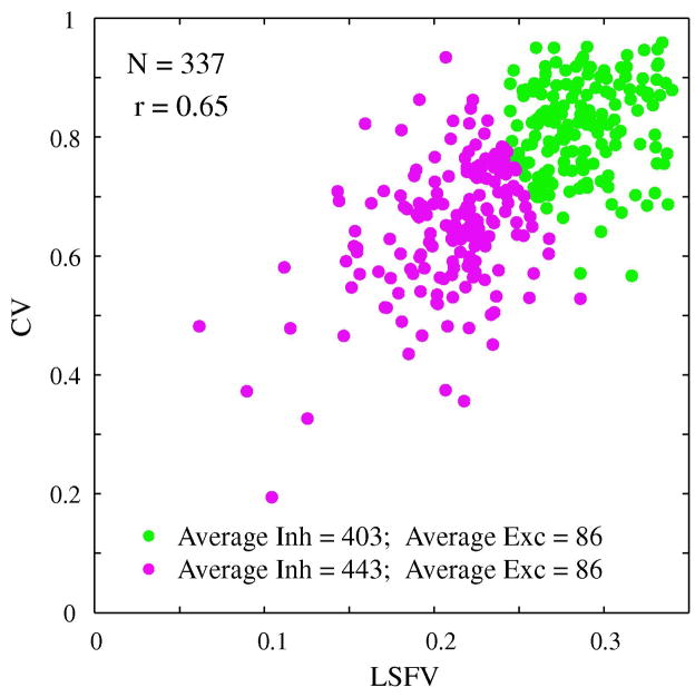
Figure 11. Correlation between orientation and spatial frequency selectivity and excitation/inhibition.

Along the linear regression line, we decomposed the set of points into two sets of roughly equal numbers of points. Then we averaged the inhibition across each of the two sets. For the upper, less- selective set the average inhibitory conductance=403 sec⁻¹ while for the lower set of higher selective points the average inhibitory conductance=443 sec⁻¹.

Then we averaged the excitation across each of the two sets. For the upper, less- selective set the average excitatory conductance=86 sec⁻¹ and the lower set of had the same average excitatory conductance=86 sec⁻¹.

A line perpendicular to the regression line divided the sub-sampled population of model simple cells approximately into two equal groups. Those cells lying to the left of and below the dividing line were the more selective group. The more selective group was colored purple and the less selective group colored green. Then we computed the mean inhibitory conductance (averaged over the fifteen runs that were used for the orientation and spatial frequency tuning curves) and averaged the inhibitory conductance across the two groups, the more and less selective. The more selective group had a higher average inhibitory conductance. When we computed the average excitations for the two groups, there was no difference. This computational result supports the idea that the common factor that controlled correlated selectivity was corticocortical inhibition.

Complex cells: feature selectivity and correlation

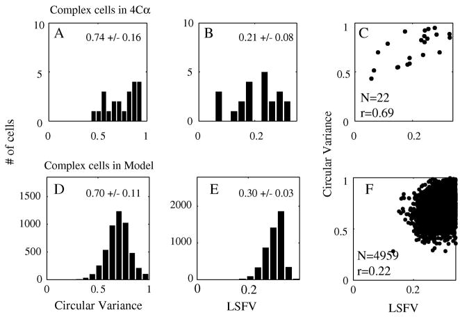
Complex cells, the cells with modulation ratio<1, tended to be less selective for orientation (Ringach et al., 2002b, Xing et al., 2004) and spatial frequency (Xing et al., 2004) throughout all layers of V1. Complex cells in layer 4Cα obeyed this rule too (Figure 12A, B). The complex cells in the large-scale model also tended to be less selective than the simple cells (Figure 12D, E). Furthermore, the correlation between orientation and spatial frequency selectivity was weaker among complex than simple cells, in the V1 4Cα data (Fig 12C) and also in the large-scale model (Fig 12F). As for the simple cells, the model’s selectivity and correlation of selectivity was less than for the data, but the tendencies were in the same direction. Previously (Zhu et al., 2009), we pointed out that the spatial frequency tuning of model complex cells depended on both inhibitory and excitatory network activity and also on the sparseness of intra-cortical excitatory-excitatory connections as implemented in this large-scale model following the lead of Tao et al. (2006). Similar reasoning applies to understanding the orientation selectivity of complex cells in layer 4C α.

Figure 12. Orientation and Spatial frequency selectivity and their correlation (Complex cells).

CV and LSFV in 4Cα complex cells (A, B) and in model complex neurons (C, D). The network model generates a correlation pattern (F) for complex cells’ orientation and spatial frequency selectivity that is similar to that seen in the data (C).

Discussion

A Mechanism for correlated spatial selectivity

In this paper we have presented a realistic model of V1 that produces orientation selectivity, spatial frequency selectivity and the correlation of selectivity similar to experimental results in V1 cortex. The major conclusion of this paper is the importance of cortical inhibition as the source of the correlation of orientation and spatial frequency selectivity in V1. As we have shown in this study, the spatial summation of LGN cells onto V1 neurons provides both orientation and spatial frequency preferences but not high selectivity (see also Zhu et al., 2009). Furthermore, the selectivity of LGN inputs is only weakly correlated in the orientation and spatial frequency domains (Fig. 6C). Therefore it is very unlikely that a strong correlation between orientation selectivity and spatial frequency selectivity is directly due to the spatial summation of LGN inputs. Our result also suggests that the correlation of orientation and spatial frequency selectivity is not mainly due to the excitation that a model neuron receives, because neurons with different selectivities, on average, receive a similar amount of excitation (Figures 8, 10, 11).

In our model the mechanism that is predominantly responsible for spatial selectivities and their correlation is intra-cortical inhibition. In the model, inhibition suppresses V1 neurons’ responses to non-optimal stimuli and generates high selectivity to orientation and spatial frequency. The variability of cortical inhibition for individual cells naturally explains the correlation of orientation and spatial frequency selectivity in the V1 population. Broadly-tuned inhibition also is the mechanism that sharpens orientation selectivity in other large-scale cortical models (McLaughlin et al., 2000, Troyer et al., 1998); we show here that local-circuit inhibition is a mechanism that can heighten selectivity in both orientation and spatial frequency domains, as was hypothesized earlier from reverse correlation data (Ringach et al., 2002a). The model’s inhibition is more broadly-tuned in orientation and stronger at low spatial frequencies than are the responses of model excitatory cells (compare Figs. 4 and 5). The predicted broader tuning of visual cortical inhibitory neurons in the orientation domain is consistent with recent experimental data (Cardin et al., 2007, Nowak et al., 2008) as is the predicted broader tuning of inhibitory neurons in the spatial frequency domain (Cardin et al., 2007).

It is important to note that the theoretical explanation offered here for spatial frequency tuning, orientation tuning, and their correlation in the visual cortex is very different from the classical picture that explains cortical spatial selectivity as a consequence of quasi-linear filtering by the neurons’ spatio-temporal receptive field (Dayan & Abbott, 2001, De Valois & De Valois, 1988, DeAngelis, Ohzawa & Freeman, 1995, Lampl, Anderson, Gillespie & Ferster, 2001, Robson, 1975). Sharpening of cortical tuning in the large-scale model we studied comes about because of nonlinear suppression caused by shunting intra-cortical inhibition. The similarity of the correlation between orientation and spatial frequency selectivity in the model and in the real cortex supports the hypothesis that, in the real cortex, spatial selectivity in different dimensions is greatly sharpened by cortical (suppressive) nonlinear inhibition. This theoretical result is similar to what was proposed from experimental results on the time-evolution of feature selectivities in the orientation (Ringach et al., 2002b, Shapley, Hawken & Ringach, 2003, Xing et al., 2005) and spatial frequency (Bredfeldt & Ringach, 2002, Ringach et al., 2002a) domains. Most other realistic cortical models have not addressed the issue of spatial frequency and orientation selectivity and their high correlation (McLaughlin et al., 2000, Tao et al., 2004, Troyer et al., 1998). One exception is the model developed by Wielaard and Sajda (2006) to study extra-classical receptive field properties of V1 neurons. The model of Wielaard and Sajda (2006) resembles our present model in that it is based on a network of conductance-based neurons in which strong inhibitory coupling leads to cortical sharpening of selectivity for orientation and spatial frequency. It is not known whether or not the Wielaard-Sajda model generates the correlation between orientation and spatial frequency selectivity we found because they did not ask this question of their model.

Finn et al (2007) revived the feedforward model to try to explain orientation selectivity. Specifically, they reported that contrast-invariant orientation selectivity could be observed in a model that includes no visually-driven inhibition but that does have a high spike threshold and variability in the membrane potential. With respect to the importance of noise and threshold, our model agrees with Finn et al (2007)’s results in that spikes in our model are evoked by fluctuations in the membrane potential and the spike threshold plays an important role in making spike rates more selective than the LGN inputs. In this way the present model also resembles the simple cell model of Wielaard et al (2001) in which neurons red spikes only when noise fluctuations caused the membrane potential to exceed threshold (Shelley et al., 2002). However, above we showed that, in the present model, high selectivity for orientation and spatial frequency was correlated with high values of inhibitory conductance. Therefore one test of our model is to test a strong prediction: that blocking local, cortical inhibition should markedly reduce spatial frequency and orientation selectivity together. This would also test Finn et al’s (2007) modified feedforward model that predicts no effect on selectivity of blocking inhibition.

It is difficult to understand how a feedforward model would explain sharpening of the cortical spatial frequency responses by selectively reducing the amplitude of response at low spatial frequency (as in Figure 2C) because the tuning mechanism in the feedforward model depends only on the amplitude of response and spike threshold, not on stimulus parameters. In our model the spatial frequency response is selectively reduced at low spatial frequency because of the strong spatial frequency responses of inhibitory neurons at low spatial frequency (as implied by the results in Figure 2, 4; further documented in Zhu et al (2009). In Zhu et al (2009) we discussed other experimental tests where our model and the model in Finn et al (2007) make different predictions.

Diversity of feature selectivity

Most theoretical work on the V1 cortical network has focused on mechanisms that can generate sharply-tuned V1 cells, However, very little work has addressed the fact that feature selectivity in V1 is very diverse even within one cortical layer, such as 4Cα. To us, the diversity of feature selectivity is as important as the feature selectivity itself. Experimental studies have shown that both orientation selectivity (Ringach et al., 2002b) and spatial frequency selectivity (Xing et al., 2004) are widely distributed in the population of macaque V1 neurons in all layers. The large-scale network model proposed in this paper generates diversity in the V1 network by variation from one cell to another in the pattern of LGN inputs and also by variation in the strength of intra-cortical synaptic interactions.

The role of local circuit inhibition in the visual cortex

The role of inhibition in the large-scale model has implications for the function of the cerebral cortex generally. Shelley et al (2002) showed that models of V1 are in a high conductance state, and this conclusion is supported again in this study (the high average conductance values in Figure 8 for instance). For the high conductance state, Shelley et al (2002) obtained the result that the time-modulated response of a model V1 neuron’s membrane potential was to a good approximation a constant plus the ratio of excitatory conductance divided by inhibitory conductance. Therefore in the model local circuit inhibition acts like shunting inhibition. Therefore, one may conclude that local circuit inhibition acts like a local divider of excitation, like a gain control. In our model, variation in the value of this gain signal across the population is what causes the variations in selectivity and induces correlations in spatial selectivity (Figs. 8–10). The conclusion that local circuit inhibition is a local gain control emerges naturally from the the model of V1 as a recurrent network in a high conductance state, justifying the assumption of a contrast gain control or normalization mechanism to fit data (Heeger, 1992). But the cortical architecture that generates the local circuit inhibition in V1 cortex is found throughout cortex, and therefore inhibition’s role throughout the cortex may be the same as it is in V1.

Modeling Considerations

We had to make a choice in the model about how spatial frequency preference or bias, induced from the LGN input, is organized spatially in the input to the model. The idea of random clusters is our interpretation of the optical imaging paper about spatial frequency maps in V1 by Sirovich and Uglesich (2004). Completely different optical imaging maps have been reported by others (Issa, Trepel & Stryker, 2000). Our judgment was that the quasi-random clustering of spatial frequency bias deduced from the maps in Sirovich and Uglesich (2004) were most consistent with the electrophysiological recording literature (DeAngelis et al., 1999). Furthermore, Xing et al. (2004) comment that there appears to be little correlation between preferred spatial frequency and the circular variance of orientation selectivity. This result also made us believe the more random maps suggested by Sirovich and Uglesich (2004). The resulting model does account for correlations between spatial selectivities in a way that makes the choice we made seem reasonable, but further experiments and modeling will be needed to validate this choice.

What took most of the theoretical effort for this paper was the exploration of different values of the ratio of recurrent cortico-cortical excitation to inhibition, S_EE/S_EI. We found that if S_EI was too weak in the model, there were not enough simple cells and the model’s spatial frequency tuning and orientation tuning distributions (as in Figure 3) were very different from the real distribution. This theoretical finding about the importance of cortico-cortical inhibition echoes physiological results that the classification of a cell as simple or complex can be changed by pharmacological manipulation of cortical inhibition (Murthy & Humphrey, 1999). The results of this paper reinforce the model’s reliance on cortico-cortical inhibition because they show that the correlation between what could be unrelated tuning parameters is quite robust and that a model with strong cortico-cortical inhibition can explain this correlation.

References

- Anderson JS, Carandini M, Ferster D. Orientation tuning of input conductance, excitation, and inhibition in cat primary visual cortex. J Neurophysiol. 2000;84(2):909–926. doi: 10.1152/jn.2000.84.2.909. [DOI] [PubMed] [Google Scholar]
- Borg-Graham LJ, Monier C, Fregnac Y. Visual input evokes transient and strong shunting inhibition in visual cortical neurons. Nature. 1998;393(6683):369–373. doi: 10.1038/30735. [DOI] [PubMed] [Google Scholar]
- Bredfeldt CE, Ringach DL. Dynamics of spatial frequency tuning in macaque V1. J Neurosci. 2002;22(5):1976–1984. doi: 10.1523/JNEUROSCI.22-05-01976.2002. [DOI] [PMC free article] [PubMed] [Google Scholar]
- Callaway EM. Local circuits in primary visual cortex of the macaque monkey. Annu Rev Neurosci. 1998;21:47–74. doi: 10.1146/annurev.neuro.21.1.47. [DOI] [PubMed] [Google Scholar]
- Campbell FW, Cooper GF, Enroth-Cugell C. The spatial selectivity of the visual cells of the cat. J Physiol. 1969;203(1):223–235. doi: 10.1113/jphysiol.1969.sp008861. [DOI] [PMC free article] [PubMed] [Google Scholar]
- Cardin JA, Palmer LA, Contreras D. Stimulus feature selectivity in excitatory and inhibitory neurons in primary visual cortex. J Neurosci. 2007;27(39):10333–10344. doi: 10.1523/JNEUROSCI.1692-07.2007. [DOI] [PMC free article] [PubMed] [Google Scholar]
- Chance FS, Nelson SB, Abbott LF. Complex cells as cortically amplified simple cells. Nat Neurosci. 1999;2(3):277–282. doi: 10.1038/6381. [DOI] [PubMed] [Google Scholar]
- Dayan P, Abbott LF. Theoretical neuroscience: computational and mathematical modeling of neural systems. Cambridge, Mass: Massachusetts Institute of Technology Press; 2001. p. xv.p. 460. [Google Scholar]
- De Valois RL, Albrecht DG, Thorell LG. Spatial frequency selectivity of cells in macaque visual cortex. Vision Res. 1982;22(5):545–559. doi: 10.1016/0042-6989(82)90113-4. [DOI] [PubMed] [Google Scholar]
- De Valois RL, De Valois KK. Spatial Vision. New York: Oxford University Press; 1988. [Google Scholar]
- DeAngelis GC, Ghose GM, Ohzawa I, Freeman RD. Functional micro-organization of primary visual cortex: receptive field analysis of nearby neurons. J Neurosci. 1999;19(10):4046–4064. doi: 10.1523/JNEUROSCI.19-10-04046.1999. [DOI] [PMC free article] [PubMed] [Google Scholar]
- DeAngelis GC, Ohzawa I, Freeman RD. Receptive-field dynamics in the central visual pathways. Trends Neurosci. 1995;18(10):451–458. doi: 10.1016/0166-2236(95)94496-r. [DOI] [PubMed] [Google Scholar]
- Enroth-Cugell C, Robson JG. The contrast sensitivity of retinal ganglion cells of the cat. J Physiol. 1966;187(3):517–552. doi: 10.1113/jphysiol.1966.sp008107. [DOI] [PMC free article] [PubMed] [Google Scholar]
- Finn IM, Priebe NJ, Ferster D. The emergence of contrast-invariant orientation tuning in simple cells of cat visual cortex. Neuron. 2007;54(1):137–152. doi: 10.1016/j.neuron.2007.02.029. [DOI] [PMC free article] [PubMed] [Google Scholar]
- Fitzpatrick D, Lund JS, Blasdel GG. Intrinsic connections of macaque striate cortex: afferent and efferent connections of lamina 4C. J Neurosci. 1985;5(12):3329–3349. doi: 10.1523/JNEUROSCI.05-12-03329.1985. [DOI] [PMC free article] [PubMed] [Google Scholar]
- Hawken MJ, Parker AJ. Contrast sensitivity and orientation selectivity in lamina IV of the striate cortex of Old World monkeys. Exp Brain Res. 1984;54(2):367–372. doi: 10.1007/BF00236238. [DOI] [PubMed] [Google Scholar]
- Hawken MJ, Parker AJ, Lund JS. Laminar organization and contrast sensitivity of direction-selective cells in the striate cortex of the Old World monkey. J Neurosci. 1988;8(10):3541–3548. doi: 10.1523/JNEUROSCI.08-10-03541.1988. [DOI] [PMC free article] [PubMed] [Google Scholar]
- Heeger DJ. Normalization of cell responses in cat striate cortex. Vis Neurosci. 1992;9(2):181–197. doi: 10.1017/s0952523800009640. [DOI] [PubMed] [Google Scholar]
- Hubel DH, Wiesel TN. Receptive fields, binocular interaction and functional architecture in the cat’s visual cortex. J Physiol. 1962;160:106–154. doi: 10.1113/jphysiol.1962.sp006837. [DOI] [PMC free article] [PubMed] [Google Scholar]
- Issa NP, Trepel C, Stryker MP. Spatial frequency maps in cat visual cortex. J Neurosci. 2000;20(22):8504–8514. doi: 10.1523/JNEUROSCI.20-22-08504.2000. [DOI] [PMC free article] [PubMed] [Google Scholar]
- Kuffler SW. Discharge patterns and functional organization of mammalian retina. J Neurophysiol. 1953;16(1):37–68. doi: 10.1152/jn.1953.16.1.37. [DOI] [PubMed] [Google Scholar]
- Lampl I, Anderson JS, Gillespie DC, Ferster D. Prediction of orientation selectivity from receptive field architecture in simple cells of cat visual cortex. Neuron. 2001;30(1):263–274. doi: 10.1016/s0896-6273(01)00278-1. [DOI] [PubMed] [Google Scholar]
- Malone BJ, Ringach DL. Dynamics of tuning in the Fourier domain. J Neurophysiol. 2008;100(1):239–248. doi: 10.1152/jn.90273.2008. [DOI] [PMC free article] [PubMed] [Google Scholar]
- Mardia KV. Statistics of directional data. London: Academic Press; 1972. [Google Scholar]
- Marino J, Schummers J, Lyon DC, Schwabe L, Beck O, Wiesing P, Obermayer K, Sur M. Invariant computations in local cortical networks with balanced excitation and inhibition. Nat Neurosci. 2005;8(2):194–201. doi: 10.1038/nn1391. [DOI] [PubMed] [Google Scholar]
- McLaughlin D, Shapley R, Shelley M, Wielaard DJ. A neuronal network model of macaque primary visual cortex (V1): orientation selectivity and dynamics in the input layer 4Calpha. Proc Natl Acad Sci U S A. 2000;97(14):8087–8092. doi: 10.1073/pnas.110135097. [DOI] [PMC free article] [PubMed] [Google Scholar]
- Mechler F, Ringach DL. On the classification of simple and complex cells. Vision Res. 2002;42(8):1017–1033. doi: 10.1016/s0042-6989(02)00025-1. [DOI] [PubMed] [Google Scholar]
- Monier C, Chavane F, Baudot P, Graham LJ, Fregnac Y. Orientation and direction selectivity of synaptic inputs in visual cortical neurons: a diversity of combinations produces spike tuning. Neuron. 2003;37(4):663–680. doi: 10.1016/s0896-6273(03)00064-3. [DOI] [PubMed] [Google Scholar]
- Movshon JA, Thompson ID, Tolhurst DJ. Spatial and temporal contrast sensitivity of neurones in areas 17 and 18 of the cat’s visual cortex. J Physiol. 1978;283:101–120. doi: 10.1113/jphysiol.1978.sp012490. [DOI] [PMC free article] [PubMed] [Google Scholar]
- Murthy A, Humphrey AL. Inhibitory contributions to spatiotemporal receptive-field structure and direction selectivity in simple cells of cat area 17. J Neurophysiol. 1999;81(3):1212–1224. doi: 10.1152/jn.1999.81.3.1212. [DOI] [PubMed] [Google Scholar]
- Nowak LG, Sanchez-Vives MV, McCormick DA. Lack of orientation and direction selectivity in a subgroup of fast-spiking inhibitory interneurons: cellular and synaptic mechanisms and comparison with other electrophysiological cell types. Cereb Cortex. 2008;18(5):1058–1078. doi: 10.1093/cercor/bhm137. [DOI] [PMC free article] [PubMed] [Google Scholar]
- Pei X, Vidyasagar TR, Volgushev M, Creutzfeldt OD. Receptive field analysis and orientation selectivity of postsynaptic potentials of simple cells in cat visual cortex. J Neurosci. 1994;14(11 Pt 2):7130–7140. doi: 10.1523/JNEUROSCI.14-11-07130.1994. [DOI] [PMC free article] [PubMed] [Google Scholar]
- Priebe NJ, Mechler F, Carandini M, Ferster D. The contribution of spike threshold to the dichotomy of cortical simple and complex cells. Nat Neurosci. 2004;7(10):1113–1122. doi: 10.1038/nn1310. [DOI] [PMC free article] [PubMed] [Google Scholar]
- Ringach DL. Spatial structure and symmetry of simple-cell receptive fields in macaque primary visual cortex. J Neurophysiol. 2002;88(1):455–463. doi: 10.1152/jn.2002.88.1.455. [DOI] [PubMed] [Google Scholar]
- Ringach DL, Bredfeldt CE, Shapley RM, Hawken MJ. Suppression of neural responses to nonoptimal stimuli correlates with tuning selectivity in macaque V1. J Neurophysiol. 2002a;87(2):1018–1027. doi: 10.1152/jn.00614.2001. [DOI] [PubMed] [Google Scholar]
- Ringach DL, Shapley RM, Hawken MJ. Orientation selectivity in macaque V1: diversity and laminar dependence. J Neurosci. 2002b;22(13):5639–5651. doi: 10.1523/JNEUROSCI.22-13-05639.2002. [DOI] [PMC free article] [PubMed] [Google Scholar]
- Robson JG. Handbook of Perception. V. New York: Academic Press; 1975. Receptive fields: neural representation of the spatial and intensive attributes of the visual image; pp. 81–116. [Google Scholar]
- Rodieck RW. Quantitative analysis of cat retinal ganglion cell response to visual stimuli. Vision Res. 1965;5(11):583–601. doi: 10.1016/0042-6989(65)90033-7. [DOI] [PubMed] [Google Scholar]
- Sceniak MP, Hawken MJ, Shapley R. Visual spatial characterization of macaque V1 neurons. J Neurophysiol. 2001;85(5):1873–1887. doi: 10.1152/jn.2001.85.5.1873. [DOI] [PubMed] [Google Scholar]
- Schummers J, Marino J, Sur M. Synaptic integration by V1 neurons depends on location within the orientation map. Neuron. 2002;36(5):969–978. doi: 10.1016/s0896-6273(02)01012-7. [DOI] [PubMed] [Google Scholar]
- Shapley R, Hawken M, Ringach DL. Dynamics of orientation selectivity in the primary visual cortex and the importance of cortical inhibition. Neuron. 2003;38(5):689–699. doi: 10.1016/s0896-6273(03)00332-5. [DOI] [PubMed] [Google Scholar]
- Shelley M, McLaughlin D, Shapley R, Wielaard J. States of high conductance in a large-scale model of the visual cortex. J Comput Neurosci. 2002;13(2):93–109. doi: 10.1023/a:1020158106603. [DOI] [PubMed] [Google Scholar]
- Sirovich L, Uglesich R. The organization of orientation and spatial frequency in primary visual cortex. Proc Natl Acad Sci U S A. 2004;101(48):16941–16946. doi: 10.1073/pnas.0407450101. [DOI] [PMC free article] [PubMed] [Google Scholar]
- Skottun BC, De Valois RL, Grosof DH, Movshon JA, Albrecht DG, Bonds AB. Classifying simple and complex cells on the basis of response modulation. Vision Res. 1991;31(7–8):1079–1086. doi: 10.1016/0042-6989(91)90033-2. [DOI] [PubMed] [Google Scholar]
- So YT, Shapley R. Spatial tuning of cells in and around lateral geniculate nucleus of the cat: X and Y relay cells and perigeniculate interneurons. J Neurophysiol. 1981;45(1):107–120. doi: 10.1152/jn.1981.45.1.107. [DOI] [PubMed] [Google Scholar]
- Tao L, Cai D, McLaughlin DW, Shelley MJ, Shapley R. Orientation selectivity in visual cortex by fluctuation-controlled criticality. Proc Natl Acad Sci U S A. 2006;103(34):12911–12916. doi: 10.1073/pnas.0605415103. [DOI] [PMC free article] [PubMed] [Google Scholar]
- Tao L, Shelley M, McLaughlin D, Shapley R. An egalitarian network model for the emergence of simple and complex cells in visual cortex. Proc Natl Acad Sci U S A. 2004;101(1):366–371. doi: 10.1073/pnas.2036460100. [DOI] [PMC free article] [PubMed] [Google Scholar]
- Troyer TW, Krukowski AE, Priebe NJ, Miller KD. Contrast-invariant orientation tuning in cat visual cortex: thalamocortical input tuning and correlation-based intracortical connectivity. J Neurosci. 1998;18(15):5908–5927. doi: 10.1523/JNEUROSCI.18-15-05908.1998. [DOI] [PMC free article] [PubMed] [Google Scholar]
- Wielaard DJ, Shelley M, McLaughlin D, Shapley R. How simple cells are made in a nonlinear network model of the visual cortex. J Neurosci. 2001;21(14):5203–5211. doi: 10.1523/JNEUROSCI.21-14-05203.2001. [DOI] [PMC free article] [PubMed] [Google Scholar]
- Wielaard J, Sajda P. Extraclassical receptive field phenomena and short-range connectivity in V1. Cereb Cortex. 2006;16(11):1531–1545. doi: 10.1093/cercor/bhj090. [DOI] [PubMed] [Google Scholar]
- Xing D, Ringach DL, Shapley R, Hawken MJ. Correlation of local and global orientation and spatial frequency tuning in macaque V1. J Physiol. 2004;557(Pt 3):923–933. doi: 10.1113/jphysiol.2004.062026. [DOI] [PMC free article] [PubMed] [Google Scholar]
- Xing D, Shapley RM, Hawken MJ, Ringach DL. Effect of stimulus size on the dynamics of orientation selectivity in Macaque V1. J Neurophysiol. 2005;94(1):799–812. doi: 10.1152/jn.01139.2004. [DOI] [PubMed] [Google Scholar]
- Zhu W, Shelley M, Shapley R. A neuronal network model of primary visual cortex explains spatial frequency selectivity. J Comput Neurosci. 2009;26(2):271–287. doi: 10.1007/s10827-008-0110-x. [DOI] [PubMed] [Google Scholar]