Penalized methods for bi-level variable selection

Abstract

In many applications, covariates possess a grouping structure that can be incorporated into the analysis to select important groups as well as important members of those groups. This work focuses on the incorporation of grouping structure into penalized regression. We investigate the previously proposed group lasso and group bridge penalties as well as a novel method, group MCP, introducing a framework and conducting simulation studies that shed light on the behavior of these methods. To fit these models, we use the idea of a locally approximated coordinate descent to develop algorithms which are fast and stable even when the number of features is much larger than the sample size. Finally, these methods are applied to a genetic association study of age-related macular degeneration.

1. INTRODUCTION

In this paper we consider regression problems in which the covariates can be grouped; our interest is in selecting important groups as well as identifying important members of these groups. We refer to this as bi-level selection. Here, we propose a new framework for thinking about grouped penalization, develop fast algorithms to fit group-penalized regression models, and apply these models to a genetic association study.

Variable selection is an important issue in regression analysis. Typically, measurements are obtained for a large number of potential predictors in order to avoid missing a potentially important link between a predictive factor and the outcome. However, to reduce variability and obtain a more interpretable model, we are often interested in selecting a smaller number of important variables.

There is a large body of available literature on the topic of variable selection, but the majority of this work is focused on the selection of individual variables. In many regression problems, however, predictors are not distinct but arise from common underlying factors. Categorical factors are often represented by a group of indicator functions; likewise for continuous factors and basis functions. Groups of measurements may be taken in the hopes of capturing unobservable latent variables or of measuring different aspects of complex entities. Some specific examples include measurements of gene expression, which can be grouped by pathway, and genetic markers, which can be grouped by the gene or haplotype that they belong to. Methods for individual variable selection may perform inefficiently in these settings by ignoring the information present in the grouping structure, or even give rise to models that are not sensible.

A common approach to variable selection is to identify the best subset of variables according to some criterion. However, this approach is unstable (Breiman, 1996) and becomes computationally infeasible as the number of variables grows to even moderate sizes. For these reasons, penalized approaches to regression have gained popularity in recent years.

In addition to penalties designed for individual variable selection such as the lasso (Tibshirani, 1996), bridge (Frank and Friedman, 1993), smoothly clipped absolute deviation penalty (SCAD, Fan and Li (2001)) and minimax concave penalty (MCP, Zhang (2007)), several methods have been developed that accommodate selection at the group level. Yuan and Lin (2006) proposed the group lasso, in which the penalty function is comprised of L₂ norms of the groups. This has the effect of encouraging sparsity at the group level while applying ridge regression-like shrinkage within a group. Meier et al. (2008) extend this idea to logistic regression, and Zhao et al. (2006) extend the idea to overlapping and hierarchical groups. These approaches perform at group level but not at an individual level variable selection. The group bridge (Huang et al., 2007), in contrast, applies a bridge penalty to the L₁ norm of the groups, performing bi-level selection by encouraging sparse solutions at the group and individual variable levels.

Group lasso and group bridge are not without their shortcomings, however. Group lasso is incapable of variable selection at the individual level and heavily shrinks large covariates. Meanwhile, group bridge suffers from a number of practical difficulties due to the fact that the bridge penalty is not everywhere differentiable. Furthermore, both methods make inflexible grouping assumptions that can cause the methods to suffer when groups are misspecified or sparsely represented.

Given the wide variety of problems that can give rise to grouped covariates, we feel that there is a need for a larger array of tools that perform bi-level selection. This paper takes two large steps towards that aim: by proposing a general framework through which the behavior of group penalties can be better understood, and by developing an efficient set of algorithms that can be used to fit models with grouped penalties.

The algorithms that have been proposed thus far to fit models with grouped penalties are either (a) inefficient for models with large numbers of predictors, or (b) limited to linear regression models, models in which the members of a group are orthogonal to each other, or both. We combine the ideas of coordinate descent optimization and local approximation of penalty functions to introduce a new, general algorithm for fitting models with grouped penalties. The resulting algorithm is stable and very fast even when the number of variables is much larger than the sample size. We apply the algorithm to models with grouped penalties, but note that the idea may be applied to other penalized regression problems in which the penalties are complicated but not necessarily grouped. We provide these algorithms as an R package, grpreg (available at http://cran.r-project.org).

In Section 2, we describe our proposed group penalization framework, show how group lasso and group bridge fit into this framework, and use the framework to motivate a new method for bi-level selection which we call group MCP. In Section 3, we discuss our computational approach to fitting group penalized models based on coordinate descent algorithms. Group lasso, group bridge, and group MCP are then compared via simulation studies in Section 4, applied to a genetic association study in Section 5, and discussed in Section 6.

2. SPECIFICATION OF MODELS WITH GROUPED PENALTIES

Suppose we have data $\left\{{({\mathbf{x}}_i,y_i)}_{i=1}^n\right\}$, where y_i is the response variable and x_i is a p-dimensional predictor containing groups that the analyst wishes to select among. We denote x_i as being composed of an unpenalized intercept and J groups x_ij, with K_j denoting the size of group j. Covariates that do not belong to a group may be thought of as a group of one. The problem of interest involves estimating a sparse vector of coefficients β using a loss function L which quantifies the discrepancy between an observation y_i and a linear predictor ${\eta }_i={{\mathbf{x}}_i}^{\prime }\beta ={\beta }_0+{\sum }_{j=1}^J{{\mathbf{x}}_{ij}}^{\prime }{\beta }_j$, where β_j represents the coefficients belonging to the j^th group.

To ensure that the penalty is applied equally, covariates are standardized prior to fitting such that ${\sum }_{i=1}^n{x}_{ijk}=0$ and $\frac{1}{n}{\sum }_{i=1}^n{x}_{ijk}^2=1\forall j,k$. We assume without loss of generality that the covariates are standardized in this way during the model fitting process and then transformed back to the original scale once all models have been fit.

2.1 Grouped penalization framework for squared error loss

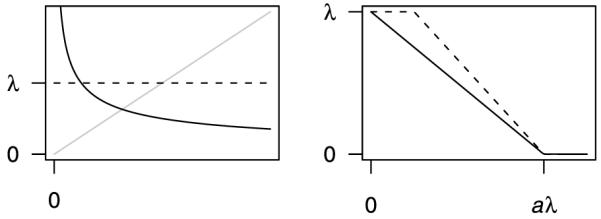
The effect of a penalty upon the solution is determined by its gradient. The derivatives of several common penalties are plotted in Fig. 1. The left panel depicts penalties of the form λβ^γ. As the plot illustrates, the ridge regression (γ = 2) rate of penalization increases with β, which has the effect of applying little to no penalization near 0 while strongly discouraging large coefficients. Meanwhile, the lasso (γ = 1) rate of penalization is constant. Finally, setting γ = 1/2 results in a rate of penalization that is very high near 0 but steadily diminishes as β grows larger.

Figure 1. Derivatives of penalty functions referenced in this paper. Left: Ridge (gray line), lasso (dashed line) and bridge (γ = 1/2, solid black line) penalties. Right: MCP (solid black line) and SCAD (dashed line) penalties.

The solution to the group lasso is defined to be the value β that minimizes the objective function

$$Q\left(\beta \right)=\frac{1}{2n}\mid \mid \mathbf{y}-\mathbf{X}\beta \mid {\mid }^2+\lambda \sum _{j=1}^J\sqrt{K_j}\mid \mid {\beta }_j\mid \mid ,$$ (1)

where ||·|| is the L₂ norm. The group bridge estimate minimizes

$$Q\left(\beta \right)=\frac{1}{2n}\mid \mid \mathbf{y}-\mathbf{X}\beta \mid {\mid }^2+\lambda \sum _{j=1}^J{K}_j^{\gamma }\mid \mid {\beta }_j\mid {\mid }_1^{\gamma },$$ (2)

where ||·||₁ is the L₁ norm. Throughout this paper, we take γ = 1/2 for group bridge.

To greater understand the action of these penalties and to illuminate the development of new ones, we can consider grouped penalties to have a form in which an outer penalty f_O is applied to a sum of inner penalties f_i. The penalty applied to a group of covariates is

$$f_O\left(\sum _{k=1}^{K_j}{f}_I(\mid {\beta }_{jk}\mid )\right)$$ (3)

and the partial derivative with respect to the jk^th covariate is

$$f_O^{\prime }\left(\sum _{k=1}^{K_j}{f}_I(\mid {\beta }_{jk}\mid )\right)f_I^{\prime }(\mid {\beta }_{jk}\mid ).$$ (4)

Note that both group lasso and group bridge fit into this framework with an outer bridge penalty; the former possesses an inner ridge penalty, while the latter has an inner lasso penalty. We have intentionally left the above framework general in the sense of not rigidly specifying the role of constants or tuning parameters such as λ, γ, or $\sqrt{K_j}$. A more specific framework would obscure the main point as well as create the potential of excluding useful forms.

From (4), we can understand group penalization to be applying a rate of penalization to a covariate that consists of two terms: the first carrying information regarding the group; the second carrying information about the individual covariate. Variables can enter the model either by having a strong individual signal or by being a member of a group with a strong collective signal. Conversely, a variable with a strong individual signal can be excluded from a model through its association with a preponderance of weak group members.

However, one must be careful not to let it oversimplify the situation. Casually combining penalties will not necessarily lead to reasonable results. For example, using the lasso as both an inner and outer penalty is equivalent to the conventional lasso, and makes no use of the grouping structure. Furthermore, properties may emerge from the combination that are more than the sum of their parts. The group lasso, for instance, possesses a convex penalty despite the fact that its outer bridge penalty is nonconvex. Nevertheless, the framework described above is a helpful lens through which to view the problem of group penalization which emphasizes the dominant feature of the method: the gradient of the penalty and how it varies over the feature space.

2.2 Group MCP

Zhang (2007) proposes a nonconvex penalty called MCP which possesses attractive theoretical properties. MCP and its derivative are defined on [0, ∞) by

$$\begin{array}{c}{f}_{\lambda ,a}\left(\theta \right)=\{\begin{array}{cc}\lambda \theta -\frac{{\theta }^2}{2a}\hfill & \text{if}\theta \le a\lambda \hfill \\ \frac{1}{2}a{\lambda }^2\hfill & \text{if}\theta >a\lambda \hfill \end{array}\phantom{\}}\hfill \\ f_{\lambda ,a}^{\prime }\left(\theta \right)=\{\begin{array}{cc}\lambda -\frac{\theta }{a}\hfill & \text{if}\theta \le a\lambda \hfill \\ 0\hfill & \text{if}\theta >a\lambda \hfill \end{array}\phantom{\}}\hfill \end{array}$$ (5)

for λ ≥ 0. The rationale behind the penalty can again be understood by considering its derivative: MCP begins by applying the same rate of penalization as the lasso, but continuously relaxes that penalization until, when θ > aλ, the rate of penalization drops to 0. MCP is motivated by and rather similar to SCAD. The connections between MCP and SCAD are explored in detail by Zhang (2007); we will briefly discuss the connections from a grouped penalty perspective in Section 6. The derivatives of MCP and SCAD are plotted in Fig. 1.

The goal of both penalties is to eliminate the unimportant variables from the model while leaving the important variables unpenalized. This would be equivalent to fitting an unpenalized model in which the truly nonzero variables are known in advance (the so-called “oracle” model). Both MCP and SCAD accomplish this asymptotically and are said to have the oracle property (Fan and Li, 2001; Zhang, 2007).

From Fig. 1, we can observe that λ is the regularization parameter that determines the magnitude of penalization and a is a tuning parameter that affects the range over which the penalty is applied. When a is small, the region in which MCP is not constant is small; when a is large, MCP penalty has a broader influence. Generally speaking, small values of a are best at retaining the unbiasedness of the MCP penalty for large coefficients, but they also run the risk of creating objective functions with problematic nonconvexity that are difficult to optimize and yield solutions that are discontinuous with respect to λ. It is therefore best to choose an a that is big enough to avoid problems but not too big. For linear regression models, when the response and covariates are standardized to have standard deviation 1, we recommend using a = 3. In our simulations, we have found this works well. It should be noted, however, that a is not scale-invariant with respect to y. If the standard deviation of the response were dramatically larger or smaller, a = 3 will not work well. As practical advice, we recommend always standardizing the variables and using a = 3. For further discussion regarding the choice of a, see Zhang (2007).

The group MCP estimate minimizes

$$Q\left(\beta \right)=\frac{1}{2n}\mid \mid \mathbf{y}-\mathbf{X}\beta \mid {\mid }^2+\sum _{j=1}^J{f}_{\lambda ,b}\left(\sum _{k=1}^{K_j}{f}_{\lambda ,a}(\mid {\beta }_{jk}\mid )\right),$$ (6)

where b, the tuning parameter of the outer penalty, is chosen to be K_jaλ/2 in order to ensure that the group level penalty attains its maximum if and only if each of its components are at their maximum. In other words, the derivative of the outer penalty reaches 0 if and only if |β_jk| ≥ aλ ∀ ∈ {1, . . . , K_j}. The relationship between group lasso, group bridge, and group MCP is illustrated for a two-covariate group in Fig. 2.

Figure 2. Penalties applied to a two-covariate group by the group lasso, group bridge, and group MCP methods. Note that where the penalty comes to a point or edge, there is the possibility that the solution will take on a sparse value; all penalties come to a point at 0, encouraging group-level sparsity, but only group bridge and group MCP allow for bi-level selection.

One can see from Fig. 2 that the group MCP penalty is capped at both the individual covariate and group levels, while the group lasso and group bridge penalties are not. This illustrates the two rationales of group MCP: (1) to avoid overshrinkage by allowing covariates to grow large, and (2) to allow groups to remain sparse internally. Group bridge allows the presence of a single large predictor to continually lower the entry threshold of the other variables in its group. This property, whereby a single strong predictor drags others into the model, prevents group bridge from achieving consistency for the selection of individual variables. Group MCP, on the other hand, limits the amount of signal that a single predictor can contribute towards the reduction of the penalty applied to the other members of the group.

2.3 Other loss functions

In generalized linear models (McCullagh and Nelder, 1999), the negative log-likelihood is used as the loss function. The usual approach to model fitting is to make a quadratic approximation to the loss function using the current estimate of the linear predictors η^(m), and update coefficients using an iteratively reweighted least squares algorithm:

$$\begin{array}{cc}\hfill L\left(\eta \right)\approx & L\left({\eta }^{\left(m\right)}\right)+{(\eta -{\eta }^{\left(m\right)})}^{\prime }\mathbf{v}\hfill \\ \hfill & +\frac{1}{2}{(\eta -{\eta }^{\left(m\right)})}^{\prime }\mathbf{W}(\eta -{\eta }^{\left(m\right)}),\hfill \end{array}$$

where v and W are the first and second derivatives of L(η) with respect to η, evaluated at η^(m). Now, letting z = η^(m)-W⁻¹v and dropping terms that are constant with respect to β, we can complete the square to obtain

$$L\left(\beta \right)\approx \frac{1}{2}{(\mathbf{z}-\mathbf{X}\beta )}^{\prime }\mathbf{W}(\mathbf{z}-\mathbf{X}\beta ).$$ (7)

For generalized linear models, W is a diagonal matrix, and the quadratic approximation renders the loss function equivalent to squared error loss in which the observations are weighted by w = diag(W). For the sake of clarity, we will present the algorithms in Section 3 primarily from the perspective of squared error loss, but mention the steps in the algorithm that are altered by iterative reweighting.

For group MCP penalties applied to logistic regression loss functions, we use the value a = 30 throughout. In logistic regression, the response variable is always on the same scale; consequently, a = 30 seems to be an appropriate value for all of the logistic regression problems we have encountered, both simulated and real.

3. LOCAL COORDINATE DESCENT

The approach that we describe for minimizing Q(β) relies on obtaining a first-order Taylor series approximation of the penalty. This approach requires continuous differentiability. Here, we treat penalties as functions of |β|; from this perspective, penalties like the lasso are continuously differentiable, with domain [0, ∞).

Coordinate descent algorithms optimize a target function with respect to a single parameter at a time, iteratively cycling through all parameters until convergence is reached. The idea is simple but efficient—each pass over the parameters requires only O(np) operations. Since the number of iterations is typically much smaller than p, the solution is reached faster even than the np² operations required to solve a linear regression problem by QR decomposition. Furthermore, since the computational burden increases only linearly with p, coordinate descent algorithms can be applied to very high-dimensional problems. Only recently has the power of coordinate descent algorithms for optimizing penalized regression problems been fully appreciated; see Friedman et al. (2007) and Wu and Lange (2008) for additional history and a fuller treatment.

Coordinate descent algorithms are ideal for problems like the lasso where deriving the solution is simple in one dimension. The group penalties discussed in this paper do not have this feature; however, one may approximate these penalties to obtain a locally accurate representation that does. The idea of obtaining approximations to penalties in order to simplify optimization of penalized likelihoods is not new. Fan and Li (2001) propose a local quadratic approximation (LQA), while Zou and Li (2008) describe a local linear approximation (LLA). The LQA and LLA algorithms can also be used to fit these models, but as we will see in Section 4, the LCD algorithm is much more efficient.

Letting β represent the current estimate of β, the overall structure of the local group coordinate descent (LCD) algorithm is as follows:

1. Choose an initial estimate $\tilde{\beta }={\beta }^{\left(0\right)}$

2. Approximate loss function, if necessary

3. Update covariates:

   1. Update ${\tilde{\beta }}_0$
   2. For j ∈ {1, . . . , J}, update ${\tilde{\beta }}_j$

4. Repeat steps 2 and 3 until convergence

First, let us consider the updating of the intercept in step (3)(a). The partial residual for updating ${\tilde{\beta }}_0$ is $\tilde{\mathbf{y}}=\mathbf{y}-{\mathbf{X}}_{-0}{\tilde{\beta }}_{-0}$, where the −0 subscript refers to what remains of X or $\tilde{\beta }$ after the 0^th column or element has been removed, respectively. The updated value of ${\tilde{\beta }}_0$ is therefore the simple linear regression solution:

$${\tilde{\beta }}_0\leftarrow \frac{{\mathbf{x}}_0^{\prime }\tilde{\mathbf{y}}}{{\mathbf{x}}_0^{\prime }{\mathbf{x}}_0}=\frac{1}{n}{\mathbf{x}}_0^{\prime }\tilde{\mathbf{y}}.$$

An equivalent but computationally more efficient way of updating ${\tilde{\beta }}_0$ is to take advantage of the current residuals $\tilde{\mathbf{r}}=\mathbf{y}-\mathbf{X}\tilde{\beta }$ (Friedman et al., 2008). Here, we note that $\tilde{\mathbf{y}}=\tilde{\mathbf{r}}+{\mathbf{x}}_0{\tilde{\beta }}_0$; thus, our update becomes

$${\tilde{\beta }}_0\leftarrow \frac{1}{n}{\mathbf{x}}_0^{\prime }\tilde{\mathbf{r}}+{\tilde{\beta }}_0.$$ (8)

Updating ${\tilde{\beta }}_0$ in this way costs only 2n operations: n operations to calculate ${\mathbf{x}}_0^{\prime }\tilde{\mathbf{r}}$ and n operations to update $\tilde{\mathbf{r}}$. In contrast, obtaining $\tilde{\mathbf{y}}$ requires n(p - 1) operations. Meanwhile, for iteratively reweighted optimization, the updating step is

$${\tilde{\beta }}_0\leftarrow {\mathbf{x}}_0^{\prime }\mathbf{W}\tilde{\mathbf{r}}∕{\mathbf{x}}_0^{\prime }\mathbf{W}{\mathbf{x}}_0+{\tilde{\beta }}_0,$$ (9)

requiring 3n operations.

Updating ${\tilde{\beta }}_j$ in step (3)(b) depends on the penalty. We discuss the updating step separately for group MCP, group bridge, and group lasso.

3.1 Group MCP

Group MCP has the most straightforward updating step. We begin by reviewing the univariate solution to the lasso. When the penalty being applied to a single parameter is λ|β|, the solution to the lasso (Tibshirani, 1996) is

$$\beta =\frac{S(\frac{1}{n}{\mathbf{x}}^{\prime }\mathbf{y},\lambda )}{\frac{1}{n}{\mathbf{x}}^{\prime }\mathbf{x}}=S\left(\frac{1}{n}{\mathbf{x}}^{\prime }\mathbf{y},\lambda \right),$$

where S(z, c) is the soft-thresholding operator (Donoho and Johnstone, 1994) defined for positive c by

$$S(z,c)=\{\begin{array}{cc}z-c\hfill & \text{if}z>c\hfill \\ 0\hfill & \text{if}\mid z\mid \le c\hfill \\ z+c\hfill & \text{if}z<-c.\hfill \end{array}\phantom{\}}$$

Group MCP does not have a similarly convenient form for updating individual parameters. However, by taking the first order Taylor series approximation about ${\tilde{\beta }}_j$, the penalty as a function of β_jk is approximately proportional to ${\tilde{\lambda }}_{jk}\mid {\beta }_{jk}\mid$, where

$${\tilde{\lambda }}_{jk}=f_{\lambda ,b}^{\prime }\left(\sum _{m=1}^{K_j}{f}_{\lambda ,a}(\mid {\tilde{\beta }}_{jm}\mid )\right)f_{\lambda ,a}^{\prime }(\mid {\tilde{\beta }}_{jk}\mid )$$ (10)

and f, f’ were defined in equation (5). Thus, in the local region where the penalty is well-approximated by a linear function, step (3)(b) consists of simple updating steps based on the soft-thresholding cutoff ${\tilde{\lambda }}_{jk}$: for k ∈ {1, . . . , K_j},

$${\tilde{\beta }}_{jk}\leftarrow S\left(\frac{1}{n}{\mathbf{x}}_{jk}^{\prime }\tilde{\mathbf{r}}+{\tilde{\beta }}_{jk},{\tilde{\lambda }}_{jk}\right)$$ (11)

or, when weights are present,

$${\tilde{\beta }}_{jk}\leftarrow \frac{S\left(\frac{1}{n}{\mathbf{x}}_{jk}^{\prime }\mathbf{W}\tilde{\mathbf{r}}+\frac{1}{n}{\mathbf{x}}_{jk}^{\prime }{\mathbf{Wx}}_{jk}{\tilde{\beta }}_{jk},{\tilde{\lambda }}_{jk}\right)}{\frac{1}{n}{\mathbf{x}}_{jk}^{\prime }{\mathbf{Wx}}_{jk}}.$$ (12)

3.2 Group bridge

The local coordinate descent algorithm for group bridge is rather similar to that for group MCP, only with

$${\tilde{\lambda }}_{jk}={\lambda }_{\gamma }{K}_j^{\gamma }\mid \mid {\tilde{\beta }}_j\mid {\mid }_1^{\gamma -1}.$$ (13)

The difficulty posed by group bridge is that, because the bridge penalty is not everywhere differentiable, ${\tilde{\lambda }}_{jk}$ is undefined at ${\tilde{\beta }}_j=0$ for γ < 1. This is not a problem caused by the algorithm; 0 presents a fundamental issue with the penalty itself. For any positive value of λ, 0 is a local minimum of the group bridge penalty. Clearly, this complicates optimization. Our approach is to begin with an initial value away from 0 and, if ${\tilde{\beta }}_j$ reaches 0 at any point during the iteration, to restrain ${\tilde{\beta }}_j$ at 0 thereafter. Obviously, this incurs the potential drawback of dropping groups that would prove to be nonzero when the solution converges. There are alternatives to this approach, such as adding a small constant to ${\tilde{\beta }}_j$ in (13). However, doing so would prevent the algorithm from taking advantage of sparsity and greatly reduce computational efficiency for large, sparse problems. In comparing the algorithm we propose with this alternative, we did not observe a large enough difference in the quality of the fitted models to justify the increase in computational burden.

3.3 Group lasso

Updating is more complicated in the group lasso because of its sparsity properties: group members go to 0 all at once or not at all. Thus, we must update ${\tilde{\beta }}_j$ at step (3)(b) in two steps: first, check whether ${\tilde{\beta }}_j=0$ and second, if $\tilde{\beta }\ne 0$, update ${\tilde{\beta }}_{jk}$ for k ∈ {1, . . . , K_j}.

The first step is performed by noting that ${\tilde{\beta }}_j\ne 0$ if and only if

$$\frac{1}{n}\mid \mid {\mathbf{X}}_j^{\prime }\tilde{\mathbf{r}}+{\mathbf{X}}_j^{\prime }{\mathbf{X}}_j{\tilde{\beta }}_j\mid \mid >\sqrt{K_j}\lambda .$$ (14)

The logic behind this condition is that if β_j cannot move in any direction away from 0 without increasing the penalty more than the movement improves the fit, then 0 is a local minimum; since the group lasso penalty is convex, 0 is also the unique global minimum. The conditions defined by (14) are in fact the Karush-Kuhn-Tucker conditions for this problem, and were first pointed out by Yuan and Lin (2006).

If this condition does not hold, then we can set ${\tilde{\beta }}_j=0$ and move on. Otherwise, we once again make a local approximation to the penalty and update the members of group j. However, instead of approximating the penalty as a function of |β_jk|, for group lasso we can obtain a better approximation by considering the penalty as a function of ${\beta }_{jk}^2$. Now, the penalty applied to β_jk may be approximated by ${\tilde{\lambda }}_{jk}{\beta }_{jk}^2∕2$, where

$${\tilde{\lambda }}_{jk}=\frac{\lambda \sqrt{K_j}}{\mid \mid {\tilde{\beta }}_j\mid \mid }.$$ (15)

This approach yields a shrinkage updating step instead of a soft-thresholding step:

$${\tilde{\beta }}_{jk}\leftarrow \frac{\frac{1}{n}{\mathbf{x}}_{jk}^{\prime }\tilde{\mathbf{r}}+{\tilde{\beta }}_{jk}}{1+{\tilde{\lambda }}_{jk}}$$ (16)

or, for weighted optimization,

$${\tilde{\beta }}_{jk}\leftarrow \frac{\frac{1}{n}{\mathbf{x}}_{jk}^{\prime }\mathbf{W}\tilde{\mathbf{r}}+\frac{1}{n}{\mathbf{x}}_{jk}^{\prime }{\mathbf{Wx}}_{jk}{\tilde{\beta }}_{jk}}{\frac{1}{n}{\mathbf{x}}_{jk}^{\prime }{\mathbf{Wx}}_{jk}+{\tilde{\lambda }}_{jk}}.$$ (17)

Note that, like (13), (15) is undefined at 0. Unlike group bridge, however, this is merely a minor algorithmic inconvenience. The penalty is differentiable; its partial derivatives simply have a different form at 0. This issue can be avoided by adding a small positive quantity δ to the denominator in equation (15).

It should be noted that Meier et al. (2008) have also proposed a coordinate descent algorithm for fitting group lasso models, and several of the ideas above are similar to ones they present. However, Meier et al. (2008) consider only the special case in which groups are orthonormal, whereas we present a more general algorithm.

3.4 Convergence of the LCD algorithm

Let β^(m) denote the value of the coefficients at a given step of the algorithm, and let β^(m+1) be the value after the next updating step has occurred. With the exception of the sparsity check during the first stage of the group lasso algorithm, β^(m+1) and β^(m) will differ by, at most, one element.

Proposition 1

At every step of the algorithms described in Sections 3.1–3.3,

$$Q\left({\beta }^{(m+1)}\right)\le Q\left({\beta }^{\left(m\right)}\right)$$ (18)

Thus, all three algorithms decrease the objective function at every step and therefore are guaranteed to converge.

This result follows from the general theory of MM (majorization-minimization) algorithms (Lange et al., 2000). A function h is said to majorize a function g if h(x) ≥ g(x) ∀x and there exists a point x* such that h(x*) = g(x*). All that remains to prove the proposition is to show that the approximations referred to by (10), (13), and (15) majorize their respective penalty functions. This is straightforward for group bridge and group MCP, as both penalties are concave on [0, ∞). They are therefore majorized by any tangent line. For group lasso, one can demonstrate majorization through inspection of second derivatives by observing that h”(β_jk) - g”(β_jk) ≥ 0 on (0, ∞).

The LCD algorithm is therefore stable and guaranteed to converge, although not necessarily to the global minimum of the objective function. The group bridge and group MCP penalty functions are nonconvex; group bridge always contains local minima and group MCP may have them as well. Furthermore, coordinate descent algorithms for penalized squared error loss functions are guaranteed to converge to minima only when the penalties are separable. Group penalties are separable between groups, but not within them. Convergence to a minimum cannot be guaranteed, then, for the one-at-a-time updates that we propose here. Nevertheless, we have not observed this to be a significant problem in practice. Comparing the convergence of the LCD algorithms to LQA/LLA algorithms (which update all parameters simultaneously) for the same data, the algorithms rarely converge to different values, and when they do, the differences are quite small.

3.5 Pathwise optimization and initial values

The local coordinate descent algorithm requires an initial value β⁽⁰⁾. Usually, we are interested in obtaining β̂ not just for a single value of λ, but for a range of values and then applying some criterion to choose an optimal λ.

Usually, the range of λ values one is interested in extends from a maximum value λ_max for which all penalized coefficients are 0 down to λ = 0 or to a minimum value λ_min at which the model becomes excessively large or ceases to be identifiable. The estimated coefficients vary continuously with λ and produce a path of solutions regularized by λ. Example coefficient paths for group lasso, group bridge, and group MCP over a fine grid of λ values are presented in Fig. 3; inspecting the path of solutions produced by a penalized regression method is often a very good way to gain insight into the methodology.

Figure 3. Coefficient paths from 0 to λ_max for group lasso, group bridge, and group MCP for a simulated data set featuring two groups, each with three covariates. In the underlying model, the solid line group has two covariates equal to 1 and the other equal to 0; the dotted line group has two coefficients equal to 0 and the other equal to −1.

Figure 3 reveals much about the behavior of grouped penalties. In particular, we note the following. (1) Even though each of the nonzero coefficients is of the same magnitude, the coefficients from the more significant solid group enter the model much more easily than the lone nonzero coefficient from the dashed group. (2) This phenomenon is less pronounced for group MCP, as it makes weaker assumptions about grouping. (3) For group MCP at λ ≈ 0.4, all of the variables with true zero coefficients have been eliminated while the remaining coefficients are unpenalized. In this region, the group MCP approach is performing as well as the oracle model. (4) In general, the coefficient paths for these group penalization methods are continuous, but are not piecewise linear, unlike those for the lasso.

Because the paths are continuous, a reasonable approach to choosing initial values is to start at one extreme of the path and use the estimate β̂ from the previous value of λ as the initial value for the next value of λ.

For group MCP and group lasso (and in general for any penalty function that is differentiable at 0), we can easily determine λ_max, the smallest value for which all penalized coefficients are 0. From (14), it is clear that

$${\lambda }_{\max }=\underset{j}{\max }\frac{\mid \mid {{\mathit{X}}_j^{\ast }}^{\prime }\tilde{\mathbf{r}}\mid \mid }{n\sqrt{K_j}},$$

where the current residuals and likelihood approximation (if necessary) are obtained using a regression fit to the intercept-only model. For group MCP,

$${\lambda }_{\max }=\underset{j,k}{\max }\sqrt{\frac{\mid {\mathbf{x}}_{jk}^{\prime }\tilde{\mathbf{r}}\mid }{n}}.$$

For these methods, we can start at λ_max using β⁽⁰⁾ = 0 and proceed towards λ_min.

This approach does not work for group bridge, however, because $\tilde{\beta }$ must be initialized away from 0. We must therefore start at λ_min and proceed toward λ_max (i.e., work in the opposite direction as group MCP and group lasso). For the initial value at λ_min, we suggest using the unpenalized univariate regression coefficients.

For all the numerical results in this paper, we follow the approach of Friedman et al. (2008) and compute solutions along a grid of 100 λ values that are equally spaced on the log scale.

3.6 Regularization parameter selection

Once a regularization path has been fit, we are typically interested in selecting an optimal point along the path. Three widely used criteria are:

$$AIC\left(\lambda \right)=2L_{\lambda }+2d{f}_{\lambda },$$ (19)

$$BIC\left(\lambda \right)=2L_{\lambda }+\log \left(n\right)d{f}_{\lambda },$$ (20)

and

$$GCV\left(\lambda \right)=\frac{2L_{\lambda }}{{[1-(d{f}_{\lambda }∕n)]}^2},$$ (21)

where df_λ is the effective number of parameters. The optimal value of λ is chosen to be the one that minimizes the criterion.

We propose the following estimator for df_λ. Let β̂ denote the fitted value of β_jk and ${\widehat{\beta }}_{jk}^{\ast }$ denote the unpenalized fit to the partial residual: ${\widehat{\beta }}_{jk}^{\ast }={\mathbf{x}}_{jk}^{\prime }\tilde{\mathbf{y}}∕n$. Then

$$\widehat{d}{f}_{\lambda }=\sum _{j=1}^J\sum _{k=1}^{K_j}\frac{{\widehat{\beta }}_{jk}}{{\widehat{\beta }}_{jk}^{\ast }}.$$ (22)

This estimator is attractive for a number of reasons. For linear fitting methods such that ŷ = Sy, there are several justifications for choosing d̂f = trace(S) (Hastie et al., 2001). Ridge regression is an example of a linear fitting method in which S = X(X’X + λI)⁻¹X’. For the special case of an orthonormal design, (22) is equal to the trace of S. The estimator also has an intuitive justification, in that it makes a smooth transition from an unpenalized coefficient with df = 1 to a coefficient that has been eliminated with df = 0. Another attractive feature is convenience: the estimator is obtained as a byproduct of the coordinate descent algorithm with no additional calculation.

Yuan and Lin (2006) propose an estimator for the effective number of parameters of the group lasso, but it involves the ordinary least squares estimator, which is undefined in high dimensions, so we do not consider it here. Another common approach is to set d̂f equal to the number of nonzero elements of β̂ (Efron et al., 2004; Zou et al., 2007). However, this has two drawbacks. One is that the estimator (and, hence, the model selection criterion) is not a continuous function of λ. The other is that this approach is inappropriate for methods that perform a heavy amount of coefficient shrinkage like the group lasso. We examine the performance of this estimator and estimator (22) using simulation studies in Section 4.

3.7 Adding an L₂ penalty

Zou and Hastie (2005) have suggested that incorporating an additional, small L₂ penalty can improve the performance of penalized regression methods, especially when the number of predictors is larger than the number of observations or when large correlation exists between the predictors. This does not pose a complication to the above algorithms. When minimizing the previously defined objective functions plus ${\lambda }_2{\sum }_{j,k}{\beta }_{jk}^2∕2$, the updating step (11) becomes

$${\tilde{\beta }}_{jk}\leftarrow \frac{S\left(\frac{1}{n}{\mathbf{x}}_{jk}^{\prime }\tilde{\mathbf{r}}+{\tilde{\beta }}_{jk},{\tilde{\lambda }}_{jk}\right)}{1+{\lambda }_2}$$

for group MCP and group bridge and the updating step (16) becomes

$${\tilde{\beta }}_{jk}\leftarrow \frac{\frac{1}{n}{\mathbf{x}}_{jk}^{\prime }\tilde{\mathbf{r}}+{\tilde{\beta }}_{jk}}{1+{\tilde{\lambda }}_{jk}+{\lambda }_2}$$

for group lasso. We use λ₂ = .001λ for the numerical results in Sections 4 and 5.

4. SIMULATION STUDIES

4.1 Efficiency

We will examine the efficiency of the LCD algorithm by measuring the average time to fit the entire path of solutions for group lasso, group bridge, and group MCP, as well as the lasso as a benchmark. Besides LCD, we consider the following algorithms: lars (Efron et al., 2004), the most widely used algorithm for fitting lasso paths as of this writing; glmnet (Friedman et al., 2008), a very efficient coordinate descent algorithm for computing lasso paths; glmpath (Park and Hastie, 2007), an approach to fitting lasso paths for GLMs not based on coordinate descent; and the LQA (Fan and Li, 2001) and LLA (Zou and Li, 2008) algorithms mentioned in Section 3.

We will consider three situations:

• Linear regression with n = 500, p = 200

• Logistic regression with n = 1000, p = 200

• Linear regression with n = 500, p = 2000

For the data sets with n > p, paths were computed down to λ = 0; for the p > n data sets, paths were computed down to 5% of λ_max.

The results of these efficiency trials are presented in Tables 1, 2, and 3. All entries are the average time in number of seconds, averaged over 100 randomly generated data sets.

Table 1. Linear regression with n = 500, p = 200.

Penalty	Algorithm	Average Time (s)
Lasso	glmnet	.03
Lasso	lars	.43
Group lasso	LQA	3.54
Group bridge	LLA	7.02
Group MCP	LLA	5.13
Group lasso	LCD	.63
Group bridge	LCD	.11
Group MCP	LCD	.10

Table 2. Logistic regression with n = 1000, p = 200.

Penalty	Algorithm	Average Time (s)
Lasso	glmnet	0.24
Lasso	glmpath	13.77
Group lasso	LQA	21.78
Group bridge	LLA	29.77
Group MCP	LLA	15.08
Group lasso	LCD	1.80
Group bridge	LCD	0.67
Group MCP	LCD	0.47

Table 3. Linear regression with n = 500, p = 2000. For the LQA and LLA algorithms, only one replication was performed; this is noted with an asterisk.

Penalty	Algorithm	Average Time (s)
Lasso	glmnet	1.60
Lasso	lars	22.69
Group lasso	LQA	1900.49*
Group bridge	LLA	1985.19*
Group MCP	LLA	1823.32*
Group lasso	LCD	23.00
Group bridge	LCD	1.46
Group MCP	LCD	3.47

These timings dramatically verify the efficiency of coordinate descent algorithms for high-dimensional penalized regression. The LCD algorithm is not only much faster than LLA/LQA for small p, its computational burden increases in a manner that is roughly linear with p as opposed to the polynomial increase suffered by LLA/LQA. Indeed, the LCD algorithms are, generally speaking, even faster than the LARS algorithm, a somewhat remarkable fact considering that the latter takes explicit advantage of special piecewise linearity properties of linear regression lasso paths.

Among the grouped penalties, group lasso is the slowest due to its two-step updating procedure. Group bridge was timed here to be the fastest, although this is potentially misleading. Group bridge saves time by not updating groups that reach 0 with no guarantee of converging to the true minimum. This is a weakness of the method, not a strength, although it does result in shorter computing times.

4.2 Regularization parameter selection

In this section, we will conduct a simulation study to compare the performance of our proposed estimator of the number of effective model parameters versus using the number of nonzero covariates as an estimator. In this section and the next, we study penalized linear regression and use BIC as the model selection criterion; simulations we have conducted for logistic regression and using AIC and GCV all illustrate the same basic trends.

We simulated data from the generating model

$$y_i={\mathbf{x}}_{i1}^{\prime }{\beta }_1^{\left(0\right)}+\dots +{\mathbf{x}}_{i10}^{\prime }{\beta }_{10}^{\left(0\right)}+{∊}_i,{∊}_i\stackrel{\mathrm{iid}}{~}\mathrm{N}(0,1),$$ (23)

with 100 observations and 10 groups, each of which containing 10 members (n = p = 100). We set β₄ = · · · = β₁₀ = 0, and randomly generated the elements of β₁ through β₃ in such a way as to have the models span signal-to-noise (SNR) ratios over the range (0.5, 3) in a roughly uniform manner. Data sets were generated independently 500 times. Model error was chosen as the outcome; lowess curves were fit to the results and plotted in Fig. 4. We define model error and SNR as follows:

$$\mathrm{ME}={(\widehat{\beta }-{\beta }^{\left(0\right)})}^{\prime }\mathrm{E}\left({\mathbf{xx}}^{\prime }\right)(\widehat{\beta }-{\beta }^{\left(0\right)})$$

and

$$\mathrm{SNR}=\frac{1}{{\sigma }^2}{\beta }^{{\left(0\right)}^{\prime }}\mathrm{E}\left({\mathbf{xx}}^{\prime }\right){\beta }^{\left(0\right)}.$$

Figure 4. Model error for each method after selecting λ with BIC using one of two estimators for the effective number of model parameters. Solid line: Estimator (22). Dashed line: Using number of nonzero elements of β.

As Fig. 4 illustrates, the performance of estimator (22) is similar to (perhaps slightly better than) that of counting the nonzero elements of β for group bridge and group MCP, but much better for the more ridge-like penalty group lasso. We consider this sufficient justification for the use of (22) throughout the remainder of this article; however, further study of this approach to estimating model degrees of freedom is warranted.

4.3 Performance

In this section, we will compare the performance of the group lasso, group bridge, and group MCP methods across a variety of independently generated data sets. Once again, data are generated from (23) with n = p = 100, J = 10. However, the sparsity of the underlying models varied over a range of true nonzero groups J₀ ∈ 2, 3, 4, 5 and over a range of nonzero members within a group K₀ ∈ 2, 3, . . . , 10. Furthermore, the magnitude of the coefficients was determined according to

$${\beta }_{jk}^{\left(0\right)}=ajkI(j\le J_0)I(k\le K_0),$$

where a was chosen such that the SNR of the model was approximately one (actual range from 0.84 to 1.45). This specification ensures that each model covers a spectrum of groups ranging from those with with small effects to those with large effects, and that each group contains large and small contributors.

We note the average number of groups and coefficients selected by the approaches for two representative cases in Table 4, and plot model errors in Fig. 5.

Table 4. Variables and groups selected by the group selection methods for the simulation study described in Section 4.3. The results for two representative models are reported. The total number of groups/individual variables is reported along with the number of those that were false positive (FP) and the number of truly nonzero groups that were not selected (false negatives, FN).

	Variables /group	Groups			Variables
		Selected	FP	FN	Selected	FP	FN
Generating model	3 groups, 3 variables per group
Group lasso	10.0	2.9	0.3	0.4	28.5	20.7	1.2
Group bridge	4.2	2.5	0.3	0.8	9.9	5.2	4.3
Group MCP	2.2	5.9	3.0	0.1	12.6	7.5	3.9
Generating model	3 groups, 8 variables per group
Group lasso	10.0	2.9	0.2	0.3	28.9	7.3	2.4
Group bridge	5.0	2.5	0.3	0.8	11.8	2.1	14.3
Group MCP	2.7	5.6	2.6	0.0	14.4	4.7	14.3

Figure 5. Model error simulation results. In each panel, the number of nonzero groups is indicated in the strip at the top. The x-axis represents the number of nonzero elements per group. At each tick mark, 500 data sets were generated. A lowess curve has been fit to the points and plotted.

The most striking difference between the methods is the extent to which the form of the penalty enforces grouping: group lasso forces complete grouping, group MCP encourages grouping to a rather slight extent, and group bridge is somewhere in between. This is seen most clearly by observing the average number of variables selected per group for the cases listed in Table 4. For group lasso, of course, this number is always 10. For group MCP, approximately two or three variables were selected per group, while group bridge selected four or five per group. We will address the underlying causes of this in the discussion.

Because group MCP makes rather cautious assumptions about grouping, the method performs well when there are a larger number of rather sparse groups – situations in which the underlying model exhibits less grouping. However, it suffers in comparison to the other methods when the nonzero coefficients are tightly clustered into groups as group MCP tends to select too many groups and make insufficient use of the grouping information. Group lasso exhibits the opposite trend in its performance, overshrinking individual coefficients when groups are sparsely populated.

5. GENETIC ASSOCIATION STUDY

Genetic association studies are an increasingly important tool for detecting links between genetic markers and diseases. The example that we will consider here involves data from a case-control study of age-related macular degeneration consisting of 400 cases and 400 controls. We confine our analysis to 30 genes that previous biological studies have suggested may be related to the disease. These genes contained 532 markers with acceptably low rates of missing data (< 20% no call rate) and high minor allele frequency (> 10%).

We analyzed the data with the group lasso, group bridge, and group MCP methods by considering markers to be grouped by the gene they belong to. Logistic regression models were fit assuming an additive effect for all markers (homozygous dominant = 2, heterozygous = 1, homozygous recessive = 0). Missing (“no call”) data was imputed from the nearest non-missing marker for that subject. In addition to the group penalization methods, we analyzed these data using a traditional one-at-a-time approach, in which univariate logistic regression models were fit and marker effects tested using a p < .05 cutoff. For group lasso and group bridge, using BIC to select λ resulted in the selection of the intercept-only model. Thus, more liberal model selection criteria were used for those methods: AIC for group lasso and GCV for group bridge.

To assess the performance of these methods, we computed 10-fold cross-validation error rates for the methods. For the one-at-a-time approach, predictions were made from an un-penalized logistic regression model fit to the training data using all the markers selected by individual testing. The results are presented in Table 5.

Table 5. Application of the three group penalization methods and a one-at-a-time method to a genetic association data set. The first three columns refer to the analysis of the actual data set; the last is the average test error over the 10 cross-validations.

	# of groups	# of covariates	Error rate	Test error rate
One-at-a-time	19	49	.312	.441
Group lasso	10	190	.321	.429
Group bridge	3	19	.342	.421
Group MCP	7	10	.364	.418

Table 5 strongly suggests the benefits of using group penalized models as opposed to one-at-a-time approaches: the three group penalization methods achieve lower test error rates and do so while selecting fewer groups. Although the error rates of ≈ .42 indicate that these 30 genes likely do not include SNPs that exert an overwhelming effect on an individual’s chances of developing age-related macular degeneration, the fact that they are well below 0.5 demonstrates that these genes do contain SNPs related to the disease. In particular, bi-level selection methods seem to perform quite well for these data. Group bridge identifies 3 promising genes out of 30 candidates, and group MCP achieves a similarly low test error rate while identifying 10 promising SNPs out of 532.

There are a number of important practical issues that arise in genetic association studies that are beyond the scope of this paper to address. Nearby genetic markers are linked; indeed, this is the impetus for addressing these problems using grouped penalization methods. However, genetic linkage also results in highly correlated predictors. We have observed that the choice of λ₂ for group bridge and group MCP has a noticeable impact on the SNPs selected. Furthermore, most genetic association studies are conducted on much larger scales than we have indicated here: moving from hundreds of SNPs to hundreds of thousands of SNPs presents a new challenge to both the computation and the assigning of group labels. The handling of missing data, the search for interactions, and the incorporation of non-genetic covariates are also important issues. The fact that signals from markers are known to be grouped in genetic association studies is a strong motivation for the further development of bi-level selection methods.

6. DISCUSSION

High-dimensional problems in which p exceeds n are increasingly common as automated data collection and storage becomes cheaper to obtain and easier to implement. For these problems, traditional likelihood methods break down and the need to introduce additional structure into the problem arises. Regression problems with grouped covariates are an important class of these types of problems. Furthermore, because we are often interested not only in selecting groups but in identifying the important members of groups, methods that can perform bi-level selection are needed.

This paper introduces a framework that sheds light on the behavior of grouped penalization methods, describes a fast, stable algorithm for implementing group penalty approaches to this problem, and applies them to an important application: genetic association studies. In addition, we describe a novel type of group penalty, group MCP, in which the effects of group and individual variable penalization are localized. The behavior of this penalty raises interesting questions about the nature of group penalization.

The derivatives of the bridge, SCAD, and MCP penalties were plotted in Fig. 1. Suppose there are 10 covariates in a group, one of which is large (i.e., at least aλ for MCP); what happens to the rate of penalization applied to the rest? For MCP, the group penalty drops to 9/10 of the initial rate. This produces rather weak grouping effects. By comparison, the derivative of the bridge penalty drops rapidly upon the introduction of any nonzero elements; this produces the stronger grouping effects seen in group bridge. The SCAD penalty, by contrast, might not drop at all; indeed, our work with a group SCAD method reveals that it displays even less grouping than group MCP.

The bridge penalty is attractive from the perspective of performing bi-level selection while still producing grouped solutions, but it introduces complications into the optimization process. The efficiency of the LCD algorithm provides a powerful incentive to work with penalties that are continuously differentiable; this was indeed one of the motivating factors behind the development of group MCP. To develop continuously differentiable penalties that can perform bi-level variable selection while producing strongly grouped solutions is an important next step. That these methods remain robust even when grouping is less pronounced is also desirable. This seemingly requires penalties whose derivatives look like that of the bridge penalty, but that do not suffer from a singularity at 0; to the knowledge of the authors, these tools have not yet been developed or studied.

Another area for the further development of these methods is their extension to cases in which groups may be overlapping. This case would arise, for instance, in gene expression studies where genes may be grouped by pathways that are not mutually exclusive.

Nevertheless, group lasso, group bridge, and group MCP can all be valuable tools depending on the application. Furthermore, using the LCD algorithm, these grouped penalization methods can be conveniently applied to large data sets that, not long ago, would have been deemed infeasible to analyze using penalized regression.

REFERENCES

- Breiman L. Heuristics of instability and stabilization in model selection. The Annals of Statistics. 1996;24(6):2350–2383. MR1425957. [Google Scholar]
- Donoho DL, Johnstone IM. Ideal spatial adaptation by wavelet shrinkage. Biometrika. 1994;81:425–455. MR1311089. [Google Scholar]
- Efron B, Hastie T, Johnstone I, Tibshirani R. Least angle regression. The Annals of Statistics. 2004;32(2):407–499. MR2060166. [Google Scholar]
- Fan J, Li R. Variable selection via nonconcave penalized likelihood and its oracle properties. Journal of the American Statistical Association. 2001;96(456):1348–1360. MR1946581. [Google Scholar]
- Frank IE, Friedman JH. A statistical view of some chemometrics regression tools (Disc: P136-148) Technometrics. 1993;35:109–135. [Google Scholar]
- Friedman J, Hastie T, Hofling H, Tibshirani R. Pathwise coordinate optimization. The Annals of Applied Statistics. 2007;1(2):302–332. MR2415737. [Google Scholar]
- Friedman J, Hastie T, Tibshirani R. Regularization paths for generalized linear models via coordinate descent. 2008 http://www-stat.stanford.edu/~hastie/Papers/glmnet.pdf. [PMC free article] [PubMed]
- Hastie T, Tibshirani R, Friedman JH. The Elements of Statistical Learning. Springer-Verlag Inc.; 2001. ISBN 0-387-95284-5. MR1851606. [Google Scholar]
- Huang J, Ma S, Xie H, Zhang C-H. A group bridge approach for variable selection. Department of Statistics and Actuarial Science, University of Iowa; 2007. Technical Report #376. [Google Scholar]
- Lange K, Hunter DR, Yang I. Optimization transfer using surrogate objective functions (with discussion) Journal of Computational and Graphical Statistics. 2000;9(1):1–59. MR1819865. [Google Scholar]
- McCullagh P, Nelder JA. Generalized Linear Models. Chapman & Hall Ltd.; 1999. ISBN 0-412-31760-5. MR0727836. [Google Scholar]
- Meier L, van de Geer S, Bühlmann P. The group lasso for logistic regression. Journalofthe RoyalStatistical Society, Series B: Statistical Methodology. 2008;70(1):53–71. MR2412631. [Google Scholar]
- Park MY, Hastie T. L1-regularization path algorithm for generalized linear models. Journal of the Royal Statistical Society, Series B: Statistical Methodology. 2007;69(4):659–677. MR2370074. [Google Scholar]
- Tibshirani R. Regression shrinkage and selection via the lasso. Journal of the Royal Statistical Society, Series B: Methodological. 1996;58:267–288. MR1379242. [Google Scholar]
- Wu TT, Lange K. Coordinate descent algorithms for lasso penalized regression. The Annals of Applied Statistics. 2008;2(1):224–244. doi: 10.1214/10-AOAS388. [DOI] [PMC free article] [PubMed] [Google Scholar]
- Yuan M, Lin Y. Model selection and estimation in regression with grouped variables. Journal of the Royal Statistical Society, Series B: Statistical Methodology. 2006;68(1):49–67. MR2212574. [Google Scholar]
- Zhang C-H. Penalized linear unbiased selection. Department of Statistics and Biostatistics, Rutgers University; 2007. Technical Report #2007-003. [Google Scholar]
- Zhao P, Rocha G, Yu B. Grouped and hierarchical model selection through composite absolute penalties. Department of Statistics, University of California; Berkeley: 2006. Technical Report #703. [Google Scholar]
- Zou H, Hastie T. Regularization and variable selection via the elastic net. Journal of the Royal Statistical Society, Series B: Statistical Methodology. 2005;67(2):301–320. MR2137327. [Google Scholar]
- Zou H, Hastie T, Tibshirani R. On the “degrees of freedom” of the lasso. The Annals of Statistics. 2007;35(5):2173–2192. MR2363967. [Google Scholar]
- Zou H, Li R. One-step sparse estimates in nonconcave penalized likelihood models. The Annals of Statistics. 2008;36(4):1509–1533. doi: 10.1214/009053607000000802. MR2435443. [DOI] [PMC free article] [PubMed] [Google Scholar]