

Abstract
The dynamics of viral infection spread, whether in laboratory cultures or in naturally infected hosts, reflects a coupling of biological and physical processes that remain to be fully elucidated. Biological processes include the kinetics of virus growth in infected cells while physical processes include transport of virus progeny from infected cells, where they are produced, to susceptible cells, where they initiate new infections. Mechanistic models of infection spread have been widely developed for systems where virus growth is coupled with transport of virus particles by diffusion, but they have yet to be developed for systems where viruses move under the influence of fluid flows. Recent experimental observations of flow-enhanced infection spread in laboratory cultures motivate here the development of initial continuum and discrete virus-particle models of infection spread. The magnitude of a dimensionless group, the Damköhler number, shows how parameters that characterize particle adsorption to cells, strain rates that reflect flow profiles, and diffusivities of virus particles combine to influence the spatial pattern of infection spread.
Introduction
The persistence of viral diseases such as influenza, AIDS, cancer, and the common cold depends on their spread from infected to susceptible animal or human hosts. A susceptible individual will typically become infected by direct or indirect physical contact with an infected animal or human, a process that is mediated by the transfer of virus particles shed from the infected host to cells of the skin, mucosal membranes, respiratory tract or gastrointestinal tract of the susceptible individual. At such ports of entry virus particles infect cells, reproduce within the cells, and virus progeny released from infected cells then spread to other susceptible cells, where they initiate new rounds of infection. For diverse viruses much is known about processes associated with virus amplification, including binding to and entering cells, reproduction within cells, and release of virus progeny from cells to the extracellular environment, and the modeling of virus dynamics in ‘well-mixed’ or spatially homogeneous systems has been well studied.1,2 However, when one allows for the more realistic case where virus and cells are not well-mixed, relatively little progress has been made. Specifically, it is not yet well appreciated how processes of virus reproduction couple with the physical movement of virus particles between cells to influence the dynamics of infection spread.
Model experimental systems for studying the dynamics of infection spread have to date primarily focused on expansion of plaques, macroscopic islands of cell death that are formed as the descendents of a single virus particle spread across a uniform layer of host cells. Studies on the spread of bacteriophages (viruses that infect bacteria) across a lawn of bacteria3–5 provided a foundation for mechanistic models of plaque expansion based on coupled virus amplification with virus movement by diffusion.6–8 Moreover, extension of such systems to mammalian viruses has provided an integrative approach for studying how cell–cell signaling may impact infection spread.9–11 When the movement of virus particles is by fluid flow rather than particle diffusion, then the extent of infection spread in culture systems can be significantly enhanced.12,13 Within infected host organisms such fluid flows may be associated with the physiological transport of blood or lymph, or fluid flows associated with lung or gastrointestinal functions. Although such flows are essential for the within-host spread of viruses, mechanistic models of flow-mediated infection spread have yet to be defined or developed. Moreover, recent experimental observations of infection “comets” or elongated plaques formed by the coupling of fluid flows and virus amplification14 have yet to be understood in the context of mechanistic models. Here, we begin to address these needs by writing and solving continuum and discrete (particle) models that highlight relevant parameters and dimensionless parameter groups that govern patterns of flow-enhanced infection spread.
Results and discussion
Microscale flows enhance the spread of virus infections
VSV-infected cells form comets or plaques when overlaid with liquid or solid agar, respectively, as shown in Fig. 1. Localized regions of cell death appear as white streaks or comets that point toward the center of the culture well, providing evidence for outward radial flows. The number of comets correlates with the number of infection events as detected by the conventional plaque assay (not shown), indicating that comet infections are initiated by infection of a single cell by a single virus particle. The axial dimension of the comets is 10- to 100-fold greater in length than the diameter of plaques formed during the same incubation period.
Fig. 1. Formation of comets (flow) and plaques (no flow) by vesicular stomatitis virus (VSV).

(a) Appearance of comets and plaques formed by VSV on BHK-21 cell monolayers at 15-h post-infection. (b) VSV comets and plaques on BHK cells at 14 h post-infection, visualized by immunofluorescent staining.
Microscale flows occur in standard culture wells
We monitored the behavior in water of fluorescent particles in the same culture plates and at the same liquid depth (3 mm) that we use for our standard cell and virus culture wells (diameter 35 mm). We found that the solution fluorescence within 1 mm of the wall increased relative to background over 48 h (Fig. 2(a)), indicating that the fluorescent particles concentrate at the wall, consistent with a mechanism of outward radial flow. Based on our tracking of individual particle movements near the wall we infer that the particles at this location experienced an average outward radial flow velocity of 0.14 mm h−1 (Fig. 2(b)). Among the standard cell culture plates, six-well plates have the largest wells. Our observation of radial microscale flows in these wells of diameter 35 mm, together with similar findings by others for flows in wells of diameter less than 1 mm,15 suggest that microscale flows may be common in standard culture plates that have from six to 96 wells. The mechanism(s) that drive flow have yet to be revealed. Outward radial flows can be readily generated within an evaporating droplet on a surface,16 and one might anticipate such flows arising in culture wells. However, we have found that infection comets form when liquid cultures are overlaid with a layer of mineral oil (unpublished observation), suggesting that other mechanisms, besides evaporation, cause the observed flows. For our case of water flowing across a length scale of 3 mm (fluid depth) and flow velocity of 0.14 mm h−1 we may calculate a Reynolds number for flow in a thin film, Re ≈ 10−4, well within the laminar flow regime.17
Fig. 2. Particle movements in culture wells.

(a) Concentration of fluorescent particles at the wall. One-micron particles in water were imaged from 8 to 48 h in a standard 6-well culture plate. (b) Particle tracking. Fluorescent particles were used as tracers for water flows in 6-well culture plates. Solution volumes matched those of our standard cell and virus cultures.
The magnitude of observed comet lengths in Fig. 1 were consistent with the known timing of VSV growth and our preliminary estimate of the flow velocity. During the earliest stage of comet formation viral progeny from the initial infected cell (first infection round) would be produced in about 7 h, and, following release could be carried by flow to nearby cells to adsorb and start a second round of infection. In 15 h one to two additional infection rounds should elapse. If we assume these additional infection rounds produce the observed cell death, based on an absence of crystal violet staining, then dividing our observed comet lengths (2–8 mm) by the time required for one to two more rounds (7–15 h) gives us a flow velocity that ranges from approximately 0.1 to 1 mm h−1, consistent with the 0.14 mm h−1 that we measured.
Continuum model of virus spread
Our system consists of transport and reaction processes occurring in: (1) the cell layer and (2) the flowing fluid above the cells. As a starting point for our modeling we describe initial continuum models that capture the key phenomena occurring in each of these two subsystems and the coupling between these subsystems that determines the overall system dynamics. For simplicity, we describe the modeling using a Cartesian coordinate system, where the flow axis for an isolated comet is aligned with the x-axis and the host-cell monolayer is defined by the xz plane, as shown in Fig. 3(a).
Fig. 3. Coordinate system for solute release with flow.
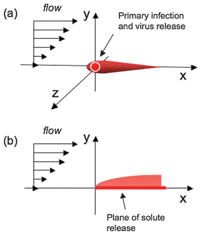
(a) Virus released at the origin is transported by flow downstream, (b) classical “Graetz–Leveque” problem of solute release from a surface in the presence of flow.
Cell-layer dynamics
Key phenomena in the cell layer are the following: binding of viruses from the fluid layer, binding of viruses from other parts of the cell layer, diffusion of virus in the interstices between cells, entry of virus into host cells, and growth and release of virus progeny into the cell layer. For these initial stages of modeling, the cell layer is treated as a homogeneous phase in which the viruses can diffuse (with a diffusivity Dvc), while the cells remain stationary. The growth of the cells is neglected, consistent with our implementation of infections at above 90% cell confluency. The kinetics of the viral infection process can be described by the following reactions:
| (1.1) |
where Vc represents free virus present in the cell layer, and host cells are either non-infected (C), infected (I), or dead (D). Here, k1 and k2 are rate constants for the corresponding elementary reactions, and Y is an average yield or burst size of virus progeny produced by each infected host cell. Assuming that the virus can move by diffusion, but the host cells cannot, we can then write coupled continuum transport/reaction expressions for each of the species:
| (2.1) |
| (2.2) |
| (2.3) |
| (2.4) |
where the brackets, [], indicate concentrations of each species, Dvc is the diffusivity of viruses in the cell phase, and is the two-dimensional Laplacian operator. Initially, [I] = [I]o at the origin and [I] = 0 away from the origin, while [C] = 0 at the origin and [C] = [C]o away from the origin, and both [Vc] and [D] = 0 at all locations. For t > 0 we have for x → ∞ that [I] = [Vc] = [D] = 0 and [C] = [C]o.
Fluid-layer dynamics
A novel aspect of the problem, relative to previous models of virus growth coupled with transport by diffusion, is the coupling between the cell-layer dynamics just described, and the transport of viruses in the flowing fluid layer covering the cell layer. The chemistry and biology occurring in the fluid layer is simpler here, but the transport is somewhat more complex. The key phenomena in the fluid layer are the following: interchange of viruses to and from the cell layer, and transport of viruses in the fluid layer via diffusion and convection by the bulk flow. Denoting the concentration of virus in the fluid phase as [Vf], the transport equation for virus in the fluid phase is given by:
| (3.1) |
where Dvf is the diffusivity of virus in the fluid layer. Eqn (2.1)–(2.4) for the cell layer are coupled to eqn (3.1) by the boundary condition that the flux of virus from the cell layer matches the flux into the fluid layer. The detailed flow profiles within culture wells are not yet known. To enable initial model development we model microscale flows for flow in a closed rectangular channel, where the velocity field ν is a standard laminar parabolic profile characterized by the channel height and the maximum fluid velocity. In the laminar flow regime the small-scale deviations from flatness of the cell-covered surface will not significantly perturb the flow. The present problem is very reminiscent of the “Graetz–Leveque” problem of classical transport phenomena. This problem and variations on it are treated in many transport phenomena texts.17–19 In the simplest version of this problem, there is flow of a fluid in the x-direction with a linear velocity profile above a surface, vx = γ̇y, with strain rate γ̇, where the wall-normal direction is y and the neutral direction is z, as shown in Fig. 3(b). For x < 0, the surface is neutral, while for x > 0 a solute rapidly dissolves from the surface into the fluid, so the concentration boundary condition at y = 0, x > 0 is c = 1. (The problem of infinitely fast adsorption from the fluid to the surface when x > 0 is equivalent upon replacing c by 1 − c.) It is well known that a concentration boundary layer develops, whose thickness δy increases as (Dx/γ̇)1/3, with diffusivity D of the solute in the fluid. In the virus model Dvf would replace D. This scaling comes from the balance of convection in the x-direction and diffusion in the y-direction and is robust with respect to the details of the problem. For example, if there is a source of chemical species at a point on the wall, while otherwise the wall is neutral, the resulting plume spreads in both the y and z directions as (Dx/γ̇)1/3. An example of a recent, detailed study of this class of problems in the context of microfluidics is given by Jensen and co-workers, who considered adsorption of chemical species on the walls of a microfluidic channel for purposes of surface-based diagnostic assays.20 The present problem is modified from the classical one in that we have both release of the species (virus) from the surface, generating a plume, and subsequent binding of the virus to healthy cells on the same surface downstream from the point of release.
The character of virus transport in the fluid phase can be characterized by the Peclet number Pe, a dimensionless number defined by:
When Pe ≫ 1, virus particles will be transported downstream by flow a distance much larger than H long before they are able to diffuse a distance H. For current conditions of interest (e.g., Vmax=1000 μmh−1, H=300 μm, Dvf=2 × 10⁻⁸ cm2 s−1) we estimate that Pe will be about 40 or larger. In this situation, one can use boundary layer scaling arguments to define basic characteristics of a “plume” of virus particles released from the cell layer at x = 0, y = 0, z = 0. These arguments apply on time scales that are short compared to the diffusion time H2/Dvf or 10 h. Specifically, the plume will spread both horizontally and vertically with a width that scales as (DvfHx/Vmax)1/3 where x is the downstream distance from the point of release of the particles. Indeed, the experimentally observed comets have a “head” whose shape can be well matched to this functional form, as shown in Fig. 4. The length of the plume after a given time telapsed will scale as . In addition, the flux of virus particles from the plume to the cell layer, which will determine the probability of infection of downstream cells, can be shown to scale (except when x is very small) as times the initial concentration of released particles. These scalings can be used to characterize the initial spread of viral infections via flow. It should be noted that although virus particles may be anisometric, especially the bullet-shaped VSV particle (180 nm × 80 nm), rotational diffusion is rapid compared to translational diffusion and convection, so the virus particles can be treated as having an isotropic effective diffusion coefficient. This assumption is also employed in estimates of VSV particle diffusivities based on light scattering measurements.21
Fig. 4. Infection plume correlates with predicted scaling behavior for early-stage comet.

For short time scales, near the initial infected cell, the predicted scaling of plume width (x1/3) to the distance downstream from the point of virus release (x) is shown here by the white line. The expression of viral genes is in the cell layer is shown in white, from Fig. 1(b).
Preliminary analysis of the model equations
The continuum modeling approach offers advantages by linking to classical methods, where magnitudes of key dimensionless numbers, such as the Reynolds and Peclet numbers, highlight the governing transport processes. This approach is also useful for identifying how a characteristic length scale, the boundary layer thickness, depends on parameters of the system. However, the experimentally observed comets show evidence of transport and infection by discrete entities that impact the detailed comet structure. Specifically, the “graininess” of the comet structure, visible in Fig. 1(b), is determined by individual virus particles undergoing flow, diffusion and infection. The stochasticity associated with these processes can be taken into account by replacing the transport equations with the appropriate stochastic differential equations (Langevin equations) for motions of individual virus particles.22,23 The virus particles are assumed to be small, rigid, and dilute in the solution, so the fluid flow affects the transport of the virus particles, but the transport of virus particles does not influence the flow.
Discrete model of virus spread
Here we model viruses as spheres of radius a = 75 nm. A simple shear flow with a strain rate of γ̇ = 0.1 s−1 is imposed in the positive x-direction. The wall-normal direction is y and the neutral (cross-stream) direction is z. A large number (N =105) of particles are placed at the origin (0, 0, 0), at time, t = 0, and allowed to diffuse. The motion of the particles is described by the Langevin equation, given by:
| (4.1) |
where is the transpose velocity gradient; in simple shear, κxy = γ̇ = Vmax/H, and all other components are zero. The Brownian displacement ζ, is described by its statistical properties
| (4.2) |
where the diffusion coefficient Dvf is given by the Stokes–Einstein relation
| (4.3) |
Here kB is Boltzmann’s constant, η is the viscosity of the fluid, and a is the radius of the virus. To model the sticking process, the particles are assumed to undergo first-order adsorption at the wall (y=0 plane). If the concentration, or equivalently, the probability density of the particles at the wall is denoted by cw, then
| (4.4) |
where kcap is the first-order reaction rate constant. The first-order reaction is realized in the simulation by modeling the probability of sticking as a Poisson process. Specifically, we consider all particles less than a distance a from the wall at time t as eligible to adsorb to the wall. The probability that one such particle will adsorb between time t and t+Δt (i.e., in one time step) is
| (4.5) |
Therefore at each time step, for each particle in the capture region, y ≤ a, that particle is removed from the simulations with probability pcap.
If we consider time spans much smaller than the diffusion time H2/Dvf, one can treat the domain as being semi-infinite in the y direction. In this situation the only relevant dimensionless number in the model is a modified Damköhler number,
| (4.6) |
where k is a “macroscopic” reaction rate constant, and is related to kcap by
| (4.7) |
and γ̇ is the strain rate of the flow. As Da → 0, the transport of the plume will approach the adsorption-free limit treated above. Simulation results are presented by varying the reaction rate constant, k, keeping all other parameters constant. The resulting Damköhler numbers range from 105 to 100 in decreasing powers of 10.
Sticking times
The fraction of adsorbed or stuck particles as a function of time for different reaction rate constants is shown in Fig. 5(a). The curves for different k values are parallel, and they collapse onto a single curve, when the time is non-dimensionalized by the rate constant, kcap, as shown in Fig. 5(b), plotting the fraction of stuck particles as a function of kcapt. Since the transport of the particles in the y-direction is only by diffusion, it follows from dimensional analysis that the fraction of stuck particles at a given time must be independent of γ̇ and thus can be written only as a function of the dimensionless time kcapt. We have observed that the curves are fit by a simple function, given by
Fig. 5. Particle sticking.
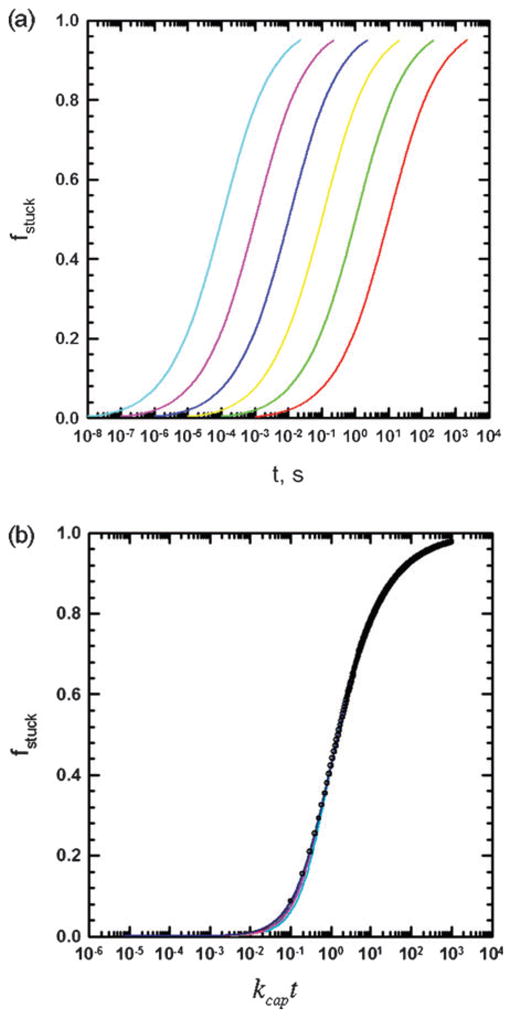
(a) Fraction of particles stuck as a function of time for Da values ranging from 105 to 100 (left to right). (b) Fraction of stuck particles plotted as a function of the dimensionless time, kcapt. Solid lines are simulation results and points are calculated using eqn (4.8).
| (4.8) |
The function in eqn (4.8) is also plotted as filled circles in Fig. 5(b).
Evolution of infection comet length
Patterns formed by stuck particles, for different values of the reaction rate constant, k, are shown in Fig. 6. The “length” of the comet was defined as the x co-ordinate of the center of mass of the stuck pattern. The x and z dimensions are normalized by the particle size, a. For large k values, the stuck particle spread appears as a circle, which increases in size with decreasing k. Below a certain value of the rate constant which corresponds to a Damköhler number of ~104, the stuck particle pattern changes to a “comet” type, with the length in the x-direction increasing with decrease in k. The shape of the head of the comet is determined by the balance of flow in the x-direction and diffusion in the z-direction, which gives rise to the relation δz ~ (Dvfx/γ̇)1/3, as described above. It should be noted that the geometry of the final pattern depends only on one dimensionless group, which in this case is the Damköhler number. Varying the Damköhler number can be accomplished by changing either one or more of the variables, k, Dvf and γ̇.
Fig. 6. Patterns formed by stuck particles.

Values for the rate of binding of the virus to the surface, corresponding to Da values 105–100 (highest value in top left, smallest value in bottom right).
Broader implications
Our analysis highlights how the interplay between reaction and transport processes will collectively influence the spatial pattern of infected cells downstream of a point source (infected cell) for release of virus particles. Here reactive processes have been defined by the irreversible adsorption or sticking of virus particles from the fluid phase to the solid surface or stationary cell monolayer downstream from their source. Transport processes are defined by uni-directional fluid flow that moves virus particles by convection and diffusion of virus particles normal to the flow direction, processes that elongate and broaden comet profiles, respectively. These effects contribute to the elongated pattern of virus spread as described by the Damköhler number in eqn (4.6). Higher Damköhler numbers, corresponding to higher sticking probabilities, lower strain rates, or lower particle diffusivities will tend to produce less elongated patterns of particle release and capture. In contrast, the extent of flow-enhanced infection spread will be increased under conditions where Damköhler numbers decrease. It should be noted that in this initial analysis we have treated reaction and transport processes as independent. It is conceivable that reactions could depend on transport processes. For example, the probability of sticking reactions could fall at sufficiently high strain rates, creating conditions where higher strain rates would have a detrimental effect on infection spread.
Through our initial development of infection-spread models we have sought to gain insights by expressing the relevant biological and physical processes in their simplest forms. In laboratory cultures and during infection spread within host organisms there will be multiple layers of additional complexity. For example, we have assumed that a fixed level or yield of particles have been instantaneously released in the presence of constant flow. In practice, an infected cell may release virus particles over a time period that is long relative to time scales for particle sticking or particle transport by flow or diffusion. We have also restricted our analysis to a single cycle of virus particle release and capture. In practice, experiments of comet formation span time scales that are long enough for captured virus particles to complete at least a second cycle of cell infection and particle release. A loss of synchrony then arises from distributions in the timing of particle sticking events that initiate new infections and distributions in the kinetics of release of new virus progeny from infected cells. In addition, yields of virus particles from individual cells may span several orders of magnitude, reflecting genetic or environmental contributions to the productivity of infected cells.24 Here, fluid flows have also been treated simply as uni-directional laminar flows parallel to a semi-infinite surface. Although the mechanism underlying the outward radial flows in the culture plates remains to be determined, flow rates in this geometry will likely depend both on radial position as well as fluid depth. Microfluidic systems that enable control of the flow conditions for infection are currently being developed.25 Additional layers of complexity will arise in physiological flows. For example, in the lung the dynamics of cilia at cell surfaces impact local mucosal flows at the cellular level as well as muco-ciliary clearance at the lung organ level, and these have been studied in great detail.26–28 Moreover, comet-like patterns of human respiratory syncytial virus infection have been observed in ciliated human airway epithelial cells.29 The flows are complex. The movement of cilia in a thin film of Newtonian periciliary fluid transfer momentum to a layer of mucus, a non-Newtonian fluid that moves as a coordinated network.30 Further, cell infection can alter the fluid balance31 as well as the ability of cells to initiate fluid motion through their cilia. Clearly, we are at a very early stage in developing a mechanistic and quantitative understanding of virus infection spread in either controlled laboratory cultures or during natural infections of host organisms.
Conclusion
Although models of infection spread have been widely developed to describe the phenomenon of plaque growth, where virus growth is coupled with virus particle movement by diffusion, models have yet to be developed where fluid flows drive virus particle movement. Here we develop initial continuum and discrete models of infection spread driven by fluid flows, and we identify governing dimensionless parameter groups that govern the formation of spatial patterns of infection spread.
Experimental methods
Cell and virus culture
Plaques and comets of vesicular stomatitis virus (VSV) were cultured on monolayers of baby hamster kidney (BHK-21) cells, as previously described.14 Briefly, plaques were formed when cultured cells were overlaid with agar while comets were formed when cells were overlaid with liquid medium. The distribution of VSV-glycoprotein (VSV-G) was visualized by indirect immunofluorescence. Rinse solution, preblock solution and block solution was made before staining. Rinse solution consisted of PBS and 0.1% saponin (Sigma). Preblock solution consisted of PBS, 0.1% saponin and 5% natal calf serum (NCS, Hyclone). Block solution consisted of PBS, 0.1% saponin, 5% NCS and 0.2% bovine serum albumin (BSA, Jackson Immunoresearch). After fixation, the agar overlay was removed and the plates were stored in PBS at 4°C. When ready to staining, monolayers were washed once with 1 ml of rinse solution and once with 1 ml of preblock solution; each wash lasted 10 min. Cells were then washed for 20 min with 1 ml of block solution to minimize the nonspecific binding. A monoclonal antibody against VSV-G (V5507, Sigma) was diluted 1: 1000 in preblock solution and 0.5 ml of the primary antibody was added to each well. After 1 h of incubation, cells were washed with rinse solution, preblock solution and block solution as before. A Cy3-conjugated affinipure F(ab′)2 fragment donkey anti-mouse antibody (Jackson Immunoresearch) was diluted 1: 300 in preblock solution. Monolayers were overlaid for 1 h in 0.5 ml of secondary antibody. After incubation, cells were washed twice with rinse solution to remove unbound antibody. Plates were stored in PBS at 4°C before imaging. During the whole process, the plates were covered with foil and put on a rotator at room temperature.
Particle flows
Red fluorescent microspheres 1.0 μm in diameter (Molecular Probes) were used as tracers to track radial flows in 6-well culture plates (Costar). The particles were diluted to a mass fraction of 10−5 (high concentration solution) or 10−7 (low concentration solution) with ultrapure water. The location of the particles was identified at 4 × magnification by a Nikon Eclipse TE300 inverted epifluorescent microscope equipped with a Prior XYZ translation stage. A monochrome SensSys 4.0 cooled CCD camera driven by MetaMorph 4.0 software (Universal Imaging) running on a Pentium II (Windows NT 4.0) captured digital images of the particles. For global measures of fluorescence change high-concentration solution was used and images were acquired every 8 h for two days. The images were analyzed by a MatLab 7.0 program, calculating intensity of light, for various times from a solution containing fluorescent microspheres versus the distance away from the vertical wall of a well. To track the movements of individual particles low-concentration solution was used and images were acquired every 10 s for an hour. The images were processed by PhotoShop 7.0 (Adobe) to optimize their brightness and contrast. The particle trajectories were mapped and velocities were measured either manually or automatically by using the software developed by Daniel Blair and Eric Dufresne (http://www.deas.harvard.edu/projects/weitzlab/matlab/). Solution volume per well and focus plane matched those of our standard comet assay.
Insight, innovation, integration
The magnitude of a single dimensionless group of biological and physical (flow) parameters is shown to govern the spread of virus infections and the work is the first to show how fluid flows may couple with virus production to impact spatial–temporal patterns of infection spread. Theory is developed to support an integrative understanding of how essential physical and biological processes combine to influence the dynamics of infection spread
Acknowledgments
This work was supported by the National Institutes of Health (AI077296 and RR023167) to J. Y., the National Science Foundation (CBET-0754573) to M. D. G., and the Graduate School of the University of Wisconsin-Madison.
References
- 1.Nowak M, May R. Virus Dynamics: Mathematical Principles of Immunology and Virology. Oxford University Press; 2000. [Google Scholar]
- 2.Perelson AS. Nat Rev Immunol. 2002;2:28. doi: 10.1038/nri700. [DOI] [PubMed] [Google Scholar]
- 3.von Angerer K. Arch F Hyg. 1924;92:312. [Google Scholar]
- 4.Adams M. Bacteriophages. Interscience Publishers; New York: 1959. [Google Scholar]
- 5.Yin J. Biochem Biophys Res Commun. 1991;174:1009. doi: 10.1016/0006-291x(91)91519-i. [DOI] [PubMed] [Google Scholar]
- 6.Koch AL. J Theor Biol. 1964;6:413. doi: 10.1016/0022-5193(64)90056-6. [DOI] [PubMed] [Google Scholar]
- 7.Yin J, McCaskill J. Biophys J. 1992;61:1540. doi: 10.1016/S0006-3495(92)81958-6. [DOI] [PMC free article] [PubMed] [Google Scholar]
- 8.Krone SM, Abedon ST. In: Bacteriophage Ecology. Abedon ST, editor. Cambridge University Press; Cambridge: 2008. [Google Scholar]
- 9.Duca KA, Lam V, Keren I, Endler EE, Letchworth GJ, Novella IS, Yin J. Biotechnol Prog. 2001;17:1156. doi: 10.1021/bp010115m. [DOI] [PubMed] [Google Scholar]
- 10.Lam V, Duca KA, Yin J. Biotechnol Bioeng. 2005;90:793. doi: 10.1002/bit.20467. [DOI] [PubMed] [Google Scholar]
- 11.Haseltine EL, Lam V, Yin J, Rawlings JB. Bull Math Biol. 2008;70:1730. doi: 10.1007/s11538-008-9316-3. [DOI] [PMC free article] [PubMed] [Google Scholar]
- 12.Appleyard G, Hapel AJ, Boulter EA. J Gen Virol. 1971;13:9. doi: 10.1099/0022-1317-13-1-9. [DOI] [PubMed] [Google Scholar]
- 13.Law M, Hollinshead R, Smith G. J Gen Virol. 2002;83:209. doi: 10.1099/0022-1317-83-1-209. [DOI] [PubMed] [Google Scholar]
- 14.Zhu Y, Yin J. J Virol Methods. 2007;139:100. doi: 10.1016/j.jviromet.2006.09.006. [DOI] [PubMed] [Google Scholar]
- 15.Rieger B, van den Doel LR, van Vliet LJ. Phys Rev E. 2003:68. doi: 10.1103/PhysRevE.68.036312. [DOI] [PubMed] [Google Scholar]
- 16.Deegan RD, Bakajin O, Dupont TF, Huber G, Nagel SR, Witten TA. Nature. 1997;389:827. doi: 10.1103/physreve.62.756. [DOI] [PubMed] [Google Scholar]
- 17.Bird RB, Stewart WE, Lightfoot EN. Transport Phenomena. J. Wiley; New York: 2002. [Google Scholar]
- 18.Deen WM. Analysis of Transport Phenomena. Oxford University Press; Oxford: 1998. [Google Scholar]
- 19.Leal LG. Laminar Flow and Convective Transport Processes: Scaling Principles and Asymptotic Analysis. Butterworth-Heinemann; New York: 1992. [Google Scholar]
- 20.Gervais T, Jensen KF. Chem Eng Sci. 2006;61:1102. [Google Scholar]
- 21.Hartford SL, Lesnaw JA, Flygare WH, MacLeod R, Reichmann ME. Proc Natl Acad Sci U S A. 1975;72:1202. doi: 10.1073/pnas.72.3.1202. [DOI] [PMC free article] [PubMed] [Google Scholar]
- 22.Gardiner C. Handbook of Stochastic Methods for Physics Chemistry and the Natural Sciences. 2. Springer-Verlag; New York: 1994. [Google Scholar]
- 23.Kloeden PE, Platen E. Numerical Solution of Stochastic Differential Equations. Springer; Berlin: 1992. [Google Scholar]
- 24.Zhu Y, Yongky A, Yin J. Virology. 2009;385:39. doi: 10.1016/j.virol.2008.10.031. [DOI] [PMC free article] [PubMed] [Google Scholar]
- 25.Zhu Y, Warrick JW, Haubert K, Beebe DJ, Yin J. Biomed Microdevices. 2009;11:565. doi: 10.1007/s10544-008-9263-7. [DOI] [PMC free article] [PubMed] [Google Scholar]
- 26.Brennen C, Winet H. Annu Rev Fluid Mech. 1977;9:339. [Google Scholar]
- 27.Sleigh MA, Blake JR, Liron N. Am Rev Respir Dis. 1988;137:726. doi: 10.1164/ajrccm/137.3.726. [DOI] [PubMed] [Google Scholar]
- 28.Houtmeyers E, Gosselink R, Gayan-Ramirez G, Decramer M. Eur Respir J. 1999;13:1177. doi: 10.1034/j.1399-3003.1999.13e39.x. [DOI] [PubMed] [Google Scholar]
- 29.Zhang L, Peeples ME, Boucher RC, Collins PL, Pickles RJ. J Virol. 2002;76:5654. doi: 10.1128/JVI.76.11.5654-5666.2002. [DOI] [PMC free article] [PubMed] [Google Scholar]
- 30.Matsui H, Randell SH, Peretti SW, Davis CW, Boucher RC. J Clin Invest. 1998;102:1125. doi: 10.1172/JCI2687. [DOI] [PMC free article] [PubMed] [Google Scholar]
- 31.Tarran R, Button B, Picher M, Paradiso AM, Ribeiro CM, Lazarowski ER, Zhang L, Collins PL, Pickles RJ, Fredberg JJ, Boucher RC. J Biol Chem. 2005;280:35751. doi: 10.1074/jbc.M505832200. [DOI] [PMC free article] [PubMed] [Google Scholar]