Enhanced sampling and applications in protein folding in explicit solvent

Abstract

We report a single-copy tempering method for simulating large complex systems. In a generalized ensemble, the method uses runtime estimate of the thermal average energy computed from a novel integral identity to guide a continuous temperature-space random walk. We first validated the method in a two-dimensional Ising model and a Lennard-Jones liquid system. It was then applied to folding of three small proteins, trpzip2, trp-cage, and villin headpiece in explicit solvent. Within 0.5∼1 microsecond, all three systems were reversibly folded into atomic accuracy: the alpha carbon root mean square deviations of the best folded conformations from the native states were 0.2, 0.4, and 0.4 Å, for trpzip2, trp-cage, and villin headpiece, respectively.

INTRODUCTION

Molecular simulations at room temperature usually suffer from a slow dynamics for large complex systems, such as proteins in explicit solvent. A promising solution to the problem is to use tempering methods, either single-copy based methods^{1, 2} such as simulated tempering, or multiple-copy based methods such as parallel tempering, also known as replica exchange.³ In either case, the system regularly changes its temperature in a way that is consistent to the underlying thermodynamics. The value of these methods lies in that they can efficiently overcome energy barriers by exploiting a fast dynamics at higher temperatures.

In traditional tempering methods, the temperature is a discrete random variable that can only assume a few predefined values. The success rate of transitions between two neighboring temperatures depends on the overlap of canonical energy distributions at the two temperatures and decays as the system size grows. Thus, to reach an optimal sampling efficiency for a large system, one needs to narrow down the temperature gap, and to increase the number of sampling temperatures. In simulated tempering, the number of weighting parameters to be estimated for simulation increases with the number of temperatures. In replica exchange, the node-node communication cost increases with the number of temperatures. Naturally, it is desirable to have an efficient tempering method that does not depend on a discrete-temperature setup.

In this paper, we report a single-copy tempering method in which the temperature is a continuous variable driven by a Langevin equation. It is based on an improved version of a previous method.² By employing improved estimators for thermodynamic quantities, one cannot only realize an efficient tempering but also correctly calculate thermodynamic quantities for the entire temperature spectrum. The essential feature of the method is the calculation of the thermal average energy $\tilde{E}\left(\beta \right)$ along the simulation trajectory. After the convergence of $\tilde{E}\left(\beta \right)$, the partition function and other thermodynamic quantities can be easily derived.

The paper is organized as follows. In Sec. 2, we give a theoretical derivation of the method. In Sec. 3, the method is verified on a two-dimensional Ising model and a Lennard-Jones liquid system, where the exact thermodynamic quantities are either known or accurately computable. In Sec. 4, we apply the method to the folding of three small proteins, trpzip2, trp-cage, and villin headpiece, in explicit solvent. The minimal alpha-carbon root mean square deviation (C_α-RMSDs) of the best folded conformations from the native states are 0.2, 0.4, and 0.4 Å, respectively (the last figure for villin headpiece is measured from an x-ray reference structure; and it should be 1.0 Å if it is measured from an NMR reference structure).

METHOD

Our method samples the system in a continuous temperature range and calculates thermodynamic properties as functions of the temperature. As we shall see, a random walk in temperature space only requires an estimate of the average energy at the current temperature in order to correctly populate the desired distribution. We present an efficient way for estimating the average energy and use it to perform a fast sampling along the temperature. In addition, an adaptive averaging scheme is used to improve convergence in early stages.

This section mainly concerns the detailed description of the method. A relatively self-contained outline is first presented in Sec. 2A. The rest of the section is organized as follows. In Sec. 2B, we review basics of sampling in a generalized ensemble where the temperature is a continuous random variable. In Secs. 2C, 2D, we present integral identities that help the ensemble to asymptotically reach the desired distribution. In Sec. 2E, we present an adaptive averaging scheme to accelerate initial convergence.

Brief outline of implementation

The method can be implemented as follows. It concerns the simulation of a system in a given temperature range (β_min,β_max) according to a predefined temperature distribution w(β), which is usually proportional to 1∕β for a molecular system (the choice is explained in Appendix C). Note, we work with the reciprocal temperature β=1∕(k_BT), where k_B is the Boltzmann constant and T is the regular temperature, β here is a variable that continuously changes within the temperature range.

In each simulation step, we first change system configuration according either to constant temperature molecular dynamics or to Monte Carlo methods. Next, we update statistics about the potential energy and then compute an estimated average energy $\tilde{E}\left(\beta \right)$. The energy fluctuation, measured from the difference between the instantaneous potential energy E and the averaged value $\tilde{E}\left(\beta \right)$ at the current temperature, determines the amount of temperature change that the system can afford to maintain the distribution of the generalized ensemble. It thus can be used to drive a temperature-space random walk in a way that preserves the underlying thermodynamics at each individual temperature. Practically, we use the following Langevin equation to guide the temperature space random walk,

$$\frac{d\left(1∕\beta \right)}{dt}=\frac{d\left(k_{B}T\right)}{dt}=E-\tilde{E}\left(\beta \right)-\frac{\partial \text{\hspace{0.17em}ln}w\left(\beta \right)}{\partial \beta }+\frac{\sqrt{2}}{\beta }\xi ,$$ (1)

where E is the current potential energy, and ξ is a Gaussian white noise that satisfies ⟨ξ(t)⋅ξ(t^′)⟩=δ(t−t^′). Note, here t is the time scale for integrating the Langevin equation, which does not necessarily coincide with the actual time in molecular dynamics. Apart from the random noise, the rate of change of the temperature is determined by the difference between the instantaneous energy E and the average energy at the current temperature $\tilde{E}\left(\beta \right)$. Thus, Eq. 1 tends to raise the temperature when the instantaneous energy E rises above the average value $\tilde{E}\left(\beta \right)$, or to lower the temperature when E falls under $\tilde{E}\left(\beta \right)$. A derivation of Eq. 1 can be found in Appendix A. In implementation, β is first converted to its reciprocal k_BT=1∕β; then k_BT is updated according to Eq. 1; finally the new β is computed from the reciprocal of the updated k_BT. We use k_BT instead of β as the variable of integration, because in this way, the magnitude from the random noise is proportional to the temperature value $\sqrt{2}∕\beta =\sqrt{2}{k}_{B}T$. The effect of the temperature change can be realized as a scaling of velocity or force in molecular dynamics. We repeat the process for each simulation step until the simulation ends.

In order to interpolate thermodynamic quantities on a continuous temperature range, we divide the entire range evenly into many small bins (β_i,β_i+1). The bin size is used for applying integral identities and is much smaller than the gap between neighboring sampling temperatures in traditional tempering methods, such as replica exchange or simulated tempering. During simulation, each bin i collects separate statistics on the potential energy and its variance along the trajectory for states with β∊(β_i,β_i+1). Statistics in different bins are later combined together to form unbiased estimates of the average energy. For a complex molecular system, the adaptive averaging in Sec. 2E can be used to improve the early convergence.

For statistical efficiency, $\tilde{E}\left(\beta \right)$, β∊(β_i,β_i+1), is not calculated from the average energy of the bin, but instead from a large temperature window (β₋,β₊) containing the bin as

$$\tilde{E}\left(\beta \right)=\sum _j\Delta {\beta }_j{⟨E⟩}_j{\varphi }_s^{\prime }\left({\beta }_j\right),$$ (2)

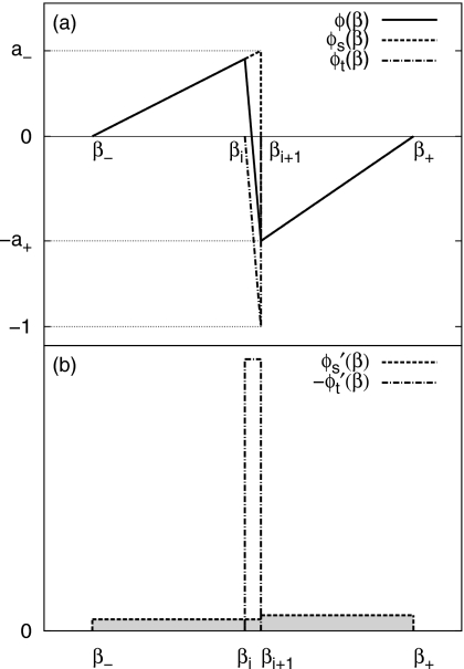
where Δβ_j=β_j+1−β_j is the bin width; ⟨E⟩_j is the average energy from the jth bin (β_j,β_j+1), ${\varphi }_s^{\prime }\left({\beta }_j\right)$ is a modulating factor to ensure an unbiased estimate, see Fig. 1b, and its computation is detailed in the next paragraph. The temperature window (β₋,β₊) is determined from the current temperature β in such a way that β is approximately at the center of the corresponding window (β₋,β₊).

Figure 1.

(a) Schematic illustration of auxiliary functions ϕ(β), ϕ_s(β) and ϕ_t(β), which are used in the integral identity for estimating the thermal average energy $\tilde{E}\left(\beta \right)$. The estimate computed in this way uses statistics from a large temperature window (β₋,β₊) instead of a single bin (β_i,β_i+1) and also avoids systematic bias. ϕ(β) is a combination of a smooth function ϕ_s(β) and a function ϕ_t(β) localized at (β_i,β_i+1). ϕ_s(β) is controlled by two parameters a₊ and a₋ that satisfy a₊+a₋=1. (b) Schematic illustration of ${\varphi }_s^{\prime }\left(\beta \right)$ and $-{\varphi }_t^{\prime }\left(\beta \right)$. ${\varphi }_s^{\prime }\left(\beta \right)$ (shaded) spans over the whole temperature window (β₋,β₊) while $-{\varphi }_t^{\prime }\left(\beta \right)$ is localized in (β_i,β_i+1).

The first step of computing $\tilde{E}\left(\beta \right)$ is to determine two parameters a₊ and a₋ by solving the following two equations:

$$a_{+}+a_{-}=1,$$ (3)

$${⟨\varphi \left({\beta }^{\prime }\right){⟨\Delta E^2⟩}_{{\beta }^{\prime }}⟩}_{\left({\beta }_{-,}{\beta }_{+}\right)}=0.$$ (4)

Here, a₊ and a₋ are parameters defined in the equation ϕ(β)=ϕ_s(β)+ϕ_t(β), whose two components ϕ_s(β) and ϕ_t(β) are defined as

$$\begin{array}{l}{\varphi }_s\left(\beta \right)=\{\begin{array}{ll}{a}_{-}\left(\beta -{\beta }_{-}\right)∕\left({\beta }_{j+1}-{\beta }_{-}\right),\hfill & \beta ∊\left({\beta }_{-},{\beta }_{i+1}\right)\hfill \\ a_{+}\left(\beta -{\beta }_{+}\right)∕\left({\beta }_{+}-{\beta }_{j+1}\right),\hfill & \beta ∊\left({\beta }_{i+1},{\beta }_{+}\right),\hfill \end{array}\phantom{\}}\\ \end{array}$$ (5)

and

$${\varphi }_t\left(\beta \right)=\{\begin{array}{ll}-\left(\beta -{\beta }_i\right)∕\left({\beta }_{i+1}-{\beta }_i\right),\hfill & \beta ∊\left({\beta }_i.{\beta }_{i+1}\right)\hfill \\ 0,\hfill & \text{otherwise},\hfill \end{array}\phantom{\}}$$ (6)

respectively. Figure 1a schematically illustrates ϕ_s(β), ϕ_t(β), and ϕ(β). In Eq. 4, the inner bracket ⟨⋯⟩_β^′ is a configuration average of the energy fluctuation ⟨ΔE²⟩_β^′ at a fixed temperature β^′. For β^′∊(β_j,β_j+1), since the bin size is small, we compute the energy fluctuation from the states collected in the bin (β_j,β_j+1), and use it to approximate ⟨ΔE²⟩_β^′. The outer angular bracket ⟨⋯⟩_(β−,β+) denotes an average over temperature β^′ within the window (β₋,β₊), it is computed as a sum of the energy fluctuation from different bins within (β₋,β₊) with ϕ(β^′) being the coefficient of combination. After the averaging, Eq. 4 is a simple linear equation of a₊ and a₋. By solving Eqs. 3, 4, a₊ and a₋ are determined. In a physical solution, both a₊ and a₋ are non-negative. If the linear equations lead to a negative value for either a₊ or a₋, zero is used instead. This measure ensures the robustness of our estimator and is thus useful in early stages when the energy fluctuation ⟨ΔE²⟩_β^′ is unreliable. The determination of a₊ or a₋ completely specifies ϕ_s(β) and its derivative ${\varphi }_s^{\prime }\left(\beta \right)$.

Generalized ensemble with a continuous temperature

We start our method by constructing a generalized ensemble in which the temperature β is a continuous variable in a given range (β_min,β_max). To sample the system correctly, we also need to make sure that the configurational distribution at a particular β is identical to that of the canonical ensemble at the same temperature. The aim of the method is to correctly populate states in the generalized ensemble and to extract thermodynamic properties for the entire temperature range.

First of all, the generalized ensemble is completely specified by an overall β-distribution p(β). Once p(β) is given, the complete distribution of atomic configuration X as well as the temperature β is also determined

$$p\left(\beta ,X\right)=\frac{\text{exp}\left[-\beta E\left(X\right)\right]}{Z\left(\beta \right)}p\left(\beta \right),$$ (7)

where E(X) is the potential energy of configuration X, and Z(β)=∫exp[−βE(X)]dX is the canonical partition function. Equation 7 is due to the requirement of preserving a canonical distribution at each temperature. It is easily verified that p(β) is recovered after we integrate p(β,X) over all configurations.

The usefulness of the joint distribution p(β,X) in Eq. 7 lies in that it specifies a temperature distribution under a fixed configuration X. For a fixed configuration X, we can perform temperature-space sampling according to p(β,X) and replace p(β) by any desired temperature distribution w(β), which is fixed during simulation, in Eq. 7. If the configurational space is sampled according to the Boltzmann distribution, the resulting overall temperature distribution after an infinitely long simulation trajectory, must be identical to the desired one w(β).

However, the exact Z(β) is usually unknown in advance. We therefore use a modified version of Eq. 7

$$p\left(\beta ,X\right)=\frac{\text{exp}\left[-\beta E\left(X\right)\right]}{\tilde{Z}\left(\beta \right)}w\left(\beta \right),$$ (8)

to conduct sampling in the temperature space, where an approximate partition function $\tilde{Z}\left(\beta \right)$ is used in place of Z(β). Note, if $\tilde{Z}\left(\beta \right)$ differs from Z(β) in Eq. 8, w(β) is no longer the overall temperature distribution, but only a parameter that specifies p(β,X), which is used in guiding the temperature-space sampling. The overall temperature distribution p(β) is calculated from integrating the joint distribution p(β,X) over configurations

$$p\left(\beta \right)=\int p\left(\beta ,X\right)dX.$$ (9)

Using Eq. 8 in Eq. 9, we have

$$p\left(\beta \right)=\frac{Z\left(\beta \right)}{\tilde{Z}\left(\beta \right)}w\left(\beta \right).$$ (10)

In simulation, $\tilde{Z}\left(\beta \right)$ is adaptively adjusted and w(β) is fixed. Therefore, the overall distribution p(β) varies according to Eq. 10. Upon convergence, $\tilde{Z}\left(\beta \right)\to Z\left(\beta \right)$, the overall temperature distribution p(β) converges to the desired one w(β).

Given a configuration X, as well as the joint distribution p(β,X) Eq. 8, sampling along the temperature can be performed by the Langevin equation Eq. 1, in which the estimated average energy $\tilde{E}\left(\beta \right)$ relates to the estimated partition function as $\tilde{E}\left(\beta \right)\equiv -\partial \text{\hspace{0.17em}ln}\tilde{Z}\left(\beta \right)∕\partial \beta$. One can demonstrate its correctness by solving the corresponding Fokker–Planck equation, see Appendix A.

The remaining task is to make sure the convergence of the estimated partition function $\tilde{Z}\left(\beta \right)$ to the correct one Z(β). As evidenced by Eq. 10, the current overall temperature distribution p(β) is close to the desired one w(β) only if the estimated the partition function $\tilde{Z}\left(\beta \right)$ is sufficiently accurate. It is interesting to note that the Langevin equation Eq. 1 does not involve the estimated partition function $\tilde{Z}\left(\beta \right)$ itself, but its derivative $\tilde{E}\left(\beta \right)$ instead. We should therefore exploit this feature and focus on a technique that adaptively improves the estimate, $\tilde{E}\left(\beta \right)$.

Unbiased estimate of a partition function

The asymptotic convergence of the partition function requires that $\tilde{Z}\left(\beta \right)$ approaches to Z(β) at any β in the range (β_min,β_max). In implementation, we divide the temperature range to many narrow bins (β_i,β_i+1). Thus we lower the requirement to that at any bin boundary β_i, $\tilde{Z}\left({\beta }_i\right)$ should equal to Z(β_i). By choosing a small bin size, we can ensure that the deviation from $\tilde{Z}\left(\beta \right)$ to Z(β) is negligible for all practical purposes. Further, to remove the dependence on a reference value of the partition function, the convergence condition is unambiguously expressed as a condition on ratios

$$\tilde{Z}\left({\beta }_i\right)∕\tilde{Z}\left({\beta }_{i+1}\right)=Z\left({\beta }_i\right)∕Z\left({\beta }_{i+1}\right).$$ (11)

Equation 11 can be rearranged as²

$${\phantom{|}\frac{Z\left(\beta \right)}{\tilde{Z}\left(\beta \right)}|}_{{\beta }_i}^{{\beta }_{i+1}}={\int }_{{\beta }_i}^{{\beta }_{i+1}}d\beta \left[\frac{d\text{\hspace{0.17em}ln}Z\left(\beta \right)}{d\beta }-\frac{d\text{\hspace{0.17em}ln}\tilde{Z}\left(\beta \right)}{d\beta }\right]\frac{Z\left(\beta \right)}{\tilde{Z}\left(\beta \right)}={\int }_{{\beta }_i}^{{\beta }_{i+1}}d\beta \left[\tilde{E}\left(\beta \right)-{⟨E⟩}_{\beta }\right]\frac{p\left(\beta \right)}{w\left(\beta \right)}={⟨\frac{\tilde{E}\left(\beta \right)-{⟨E⟩}_{\beta }}{w\left(\beta \right)}⟩}_i,$$

where we have used Eq. 10 on the second line; the inner bracket ⟨E⟩_β denotes the average energy at a particular energy β; on the last line, we convert the integral over the small temperature bin (β_i,β_i+1) to a temperature average in the same bin, as represented by the outer bracket ⟨⋯⟩_i, which is formally defined as ${⟨A⟩}_i\equiv {\int }_{{\beta }_i}^{{\beta }_{i+1}}d\beta p\left(\beta \right)A$.

During simulation, if we adaptively enforce the right hand side of the above equation to be zero, i.e.,

$${⟨\frac{\tilde{E}\left(\beta \right)}{w\left(\beta \right)}⟩}_i={⟨\frac{{⟨E⟩}_{\beta }}{w\left(\beta \right)}⟩}_i,$$ (12)

the left hand side naturally vanishes as well, i.e., $\tilde{Z}\left({\beta }_{i+1}\right)∕Z\left({\beta }_{i+1}\right)=\tilde{Z}\left({\beta }_i\right)∕Z\left({\beta }_i\right)$. In this way, the partition function as a function of the temperature can be obtained.²

We shall proceed by assuming a sufficiently small bin size and (i) $\tilde{E}\left(\beta \right)$ being a constant ${\tilde{E}}_i$ within a bin i, and correspondingly, $\text{ln}\tilde{Z}\left(\beta \right)$ varies linearly with β, and (ii) p(β)∕w(β) can be treated as a constant. Equation 12 is then simplified as

$${\tilde{E}}_i=\frac{{\int }_{{\beta }_i}^{{\beta }_{i+1}}d\beta {⟨E⟩}_{\beta }p\left(\beta \right)∕w\left(\beta \right)}{{\int }_{{\beta }_i}^{{\beta }_{i+1}}d\beta p\left(\beta \right)∕w\left(\beta \right)}\approx {⟨{⟨E⟩}_{\beta }⟩}_i,$$ (13)

and the ratio of the partition function is estimated as

$$\text{ln}\left[Z\left({\beta }_i\right)∕Z\left({\beta }_{i+1}\right)\right]={\tilde{E}}_i\Delta {\beta }_i,$$

where Δβ_i=β_i+1−β_i.

A direct implication of Eq. 13 is that one can estimate ${\tilde{E}}_i$ from averages from statistics accumulated in bin i. Such an approach (which is similar to those used in the force averaging method⁴) is, although correct, ineffective when the bin size is small because the amount of statistics within a bin shrinks with the bin size. On the other hand, a large bin size can lead to a significant deviation from the desired temperature distribution, since we assumed a constant $\tilde{E}\left(\beta \right)$ within a bin. This dilemma can be resolved by using integral identities that remove the bin size dependence.

Estimators based on integral identities

We now present a method for drawing an unbiased estimate ${\tilde{E}}_i$ from a large temperature window instead of a small temperature bin. The method removes bin size dependence by combining statistics from neighboring bins in a way that avoids systematic error. A similar technique of employing integral identities to improve statistics was previously used in improving statistical distributions.^{5, 6}

We aim at transforming the right hand side of Eq. 13 from an average over a single bin (β_i,β_i+1) to an average over a larger temperature range (β₋,β₊) that encloses the bin. To do so, we use the following integral identity:

$$0=\varphi \left(\beta \right){⟨E⟩}_{\beta }{|}_{{\beta }_{-}}^{{\beta }_{+}}={\int }_{{\beta }_{-}}^{{\beta }_{+}}d\beta {\varphi }^{\prime }\left(\beta \right){⟨E⟩}_{\beta }-{\int }_{{\beta }_{-}}^{{\beta }_{+}}d\beta \varphi \left(\beta \right){⟨\Delta E^2⟩}_{\beta },$$ (14)

where ϕ(β) is a function that vanishes at the two boundaries, i.e., ϕ(β₋)=ϕ(β₊)=0; on the second line, we convert the difference between the two boundaries to an integral within the temperature range; the identity ∂⟨E⟩_β∕∂β=−⟨ΔE²⟩_β from statistical mechanics is also used.

We choose ϕ(β) as a superposition of a smoothly varying ϕ_s(β) that spans over the entire window (β₋,β₊) and a localized function ϕ_t(β) limited within the bin (β_i.β_i+1), see Fig. 1 and Eqs. 5, 6, in which a₊ and a₋ are two non-negative parameters that sum to unity, i.e., a₊+a₋=1. Note at β=β_i+1, the sudden jump in ϕ_s(β) is exactly cancelled by that in ϕ_t(β), thus we can ignore the δ-functions in ${\varphi }_s^{\prime }\left(\beta \right)$ and ${\varphi }_t^{\prime }\left(\beta \right)$ in actual computation.

The purpose of the decomposition of ϕ(β) into ϕ_s(β) and ϕ_t(β) is to use the localized function ${\varphi }_t^{\prime }\left(\beta \right)$ to create an integral exactly equal to the right hand side of Eq. 13. In this way, the integral over the small bin is transformed to another one, but over a larger temperature window

$${\tilde{E}}_i=\frac{1}{\Delta {\beta }_i}{\int }_{{\beta }_i}^{{\beta }_{i+1}}d\beta {⟨E⟩}_{\beta }={\int }_{{\beta }_{-}}^{{\beta }_{+}}d\beta \left[{\varphi }_s^{\prime }\left(\beta \right){⟨E⟩}_{\beta }-\varphi \left(\beta \right){⟨\Delta E^2⟩}_{\beta }\right].$$ (15)

In early stages of simulation, the energy fluctuation ⟨ΔE²⟩_β in the second term of the right hand side of Eq. 15 can be unreliable for a complex system. To avoid direct inclusion of energy fluctuation, we choose the combination parameters a₊ and a₋ in such a way that the fluctuation term vanishes,

$${\int }_{{\beta }_{-}}^{{\beta }_{+}}d\beta \varphi \left(\beta \right){⟨\Delta E^2⟩}_{\beta }=0.$$ (16)

Equation 16 and a₊+a₋=1 yield a solution of a₊ and a₋, which also determines ${\varphi }_s^{\prime }\left(\beta \right)$. Thus we have,

$${\tilde{E}}_i={\int }_{{\beta }_{-}}^{{\beta }_{+}}d\beta {\varphi }_s^{\prime }\left(\beta \right){⟨E⟩}_{\beta }.$$ (17)

Since ${\varphi }_s^{\prime }\left(\beta \right)$ is a constant within a single bin, it can be factored out of the integral when integrating each individual bin. The integral is thus converted to a sum over averages,

$${\tilde{E}}_i=\sum _j{\varphi }_s^{\prime }\left({\beta }_j\right){\int }_{{\beta }_j}^{{\beta }_{j+1}}d\beta {⟨E⟩}_{\beta }=\sum _j{\varphi }_s^{\prime }\left({\beta }_j\right)\Delta {\beta }_j{⟨{⟨E⟩}_{\beta }⟩}_j.$$ (18)

A comparison with Eq. 13 shows that Eq. 18 is merely a linear combination of ${\tilde{E}}_i$’s obtained from different bins. The auxiliary function ${\varphi }_s^{\prime }\left(\beta \right)$ serves as a set of coefficients of combination, whereas Eq. 16 ensures the asymptotical convergence.

The above technique of extracting an estimate from an integral identity can be employed in computing other thermodynamic quantities, such as the average energy, heat capacity, and energy histogram. Thus, we are able to calculate these quantities at a particular temperature, even though the simulation is performed in an ensemble where the temperature is continuous.

The result for the average energy is most easily obtained. Consider a limiting case where β_i+1→β_i (with ϕ(β) modified accordingly), Eq. 15 immediately becomes an unbiased estimate of the thermal average energy ⟨E⟩_βi exactly at β_i.

Similarly, the heat capacity C_V(β) can be calculated from the energy fluctuation as β²⟨ΔE²⟩_β. The energy fluctuation at a particular temperature β is computed as

$${⟨\Delta E^2⟩}_{\beta }={\int }_{{\beta }_{-}}^{{\beta }_{+}}d{\beta }^{\prime }{\varphi }^{\prime }\left({\beta }^{\prime }\right){⟨\Delta E^2⟩}_{{\beta }^{\prime }}-{\int }_{{\beta }_{-}}^{{\beta }_{+}}d{\beta }^{\prime }\varphi \left({\beta }^{\prime }\right){⟨\Delta E^3⟩}_{{\beta }^{\prime }},$$ (19)

where we have substituted −⟨ΔE³⟩_β for ∂⟨ΔE²⟩_β∕∂β.

Estimating the energy histogram requires additional care in choosing the function ϕ(β), in order to ensure that the histogram is non-negative everywhere. It is shown in Appendix D that the optimal estimate of an energy histogram at temperature β is

$$h_{\beta }\left(E,E+\Delta E\right)\equiv {\int }_E^{E+\Delta E}{p}_{\beta }\left(E^{\prime }\right)d{E}^{\prime }\approx \frac{{\int }_{{\beta }_{-}}^{{\beta }_{+}}{\int }_E^{E+\Delta E}p\left({\beta }^{\prime },E^{\prime }\right)d{E}^{\prime }d{\beta }^{\prime }}{{\int }_{{\beta }_{-}}^{{\beta }_{+}}w\left({\beta }^{\prime }\right)\tilde{Z}\left(\beta \right)∕\tilde{Z}\left({\beta }^{\prime }\right)\text{exp}\left[-\left({\beta }^{\prime }-\beta \right)\left(E+\Delta E∕2\right)\right]d{\beta }^{\prime }},$$ (20)

where on the first line, the energy histogram h_β(E,E+ΔE) at β is defined from the constant temperature energy distribution p_β(E) at the same temperature; on the second line, it is converted to an average over the joint temperature-energy p(β,E) distribution in the generalized ensemble, which can be measured from the temperature-energy histogram in simulation trajectory. Note, for simplicity, we have assumed that the energy bin size is small compared with the energy fluctuation of a typical Boltzmann distribution. Equation 20 resembles the result from the multiple histogram method,⁷ and therefore can be treated as its counterpart in a continuous temperature ensemble.

For a quantity whose statistics are not fully accumulated during simulation (e.g., it is calculated from periodically saved trajectory snapshots after simulation), we use the following reweighting formula to obtain its value at a particular temperature β

$${⟨A⟩}_{\beta }=\frac{{\int }_{{\beta }_{-}}^{{\beta }_{+}}A\text{\hspace{0.17em}exp}\left[-\left(\beta -{\beta }^{\prime }\right)E\right]\tilde{Z}\left({\beta }^{\prime }\right)∕\tilde{Z}\left(\beta \right)d{\beta }^{\prime }}{{\int }_{{\beta }_{-}}^{{\beta }_{+}}\text{exp}\left[-\left(\beta -{\beta }^{\prime }\right)E\right]\tilde{Z}\left({\beta }^{\prime }\right)∕\tilde{Z}\left(\beta \right)d{\beta }^{\prime }},$$ (21)

where $\text{exp}\left[-\left(\beta -{\beta }^{\prime }\right)E\right]\tilde{Z}\left({\beta }^{\prime }\right)∕\tilde{Z}\left(\beta \right)$ serves as a weighting function for borrowing statistics from β^′ to β. Note, Eq. 21 is unbiased estimator even if $\tilde{Z}\left(\beta \right)$ contains error.

Adaptive averaging

We now introduce an adaptive averaging scheme for accelerating the convergence in initial stages of a simulation. Since we start from zero statistics, the error in initially estimated $\tilde{E}\left(\beta \right)$ can lead to a slow random walk in the temperature space. The adaptive averaging scheme² overcomes the problem by assigning larger weights toward recent statistics, and thus encourages a faster random walk in the temperature space.

Usually, for a statistical sample of size n, the average of a quantity A is calculated as an arithmetic mean $⟨A⟩=S_A^{\left(n\right)}∕S_1^{\left(n\right)}$, where $S_A^{\left(n\right)}={\sum }_{i=1}^n{A}_i$ is the sum of A and $S_1^{\left(n\right)}$ is the sample size n. In simulation, since statistics is collected along the trajectory, the sample size n increases as simulation progresses. To increase the weight toward recent A_i’s, we redefine $S_A^{\left(n\right)}$ and $S_1^{\left(n\right)}$ as

$$S_A^{\left(n\right)}=A_1{\gamma }^{n-1}+A_2{\gamma }^{n-2}+\cdots +A_n,$$

$$S_1^{\left(n\right)}={\gamma }^{n-1}+{\gamma }^{n-2}+\cdots +1,$$

where γ(<1) is used to gradually damp out old statistics. Such an average can be easily implemented as recursions,

$$S_A^{\left(n\right)}=\gamma S_A^{\left(n-1\right)}+A_n,$$ (22)

$$S_1^{\left(n\right)}=\gamma S_1^{\left(n-1\right)}+1.$$

However, if a constant γ is used, an average derived from Eq. 22 does not asymptotically reduce its error due to that the sample size S₁ ultimately saturates to a fixed value 1∕(1−γ). Therefore, we use

$$\gamma =1-C_{\gamma }∕n,$$ (23)

where C_γ is a numerical constant, to gradually reduce the difference between γ and 1.0. In this way, both a fast random walk in early stages and an asymptotical convergence can be achieved.

NUMERICAL RESULTS

Ising model

As the first example, we test our method on a 32×32 Ising model, which is a nontrivial system with exactly known thermodynamic properties.⁸ Results from the alternative method of estimating $\tilde{E}\left(\beta \right)$, described in Appendix B, are also included. Parameters common to the two methods were set to be the same.

The temperature range was β∊(0.35,0.55) or T=(1.818,2.857), which covered the critical temperature T≈2.27 of the phase transition, and the temperature distribution was defined by a constant w(β), or a flat-β histogram. The bin size for collecting statistics was δβ=0.0002, and thus there were 1000 bins in the entire temperature range. For each temperature bin (β_i,β_i+1), the temperature window for applying integral identities was given by (β₋,β₊)=(β_i−Δβ,β_i+1+Δβ) with Δβ=0.02 in evaluating Eq. 18; thus 201 bins were included in a window (except at temperatures near the boundaries, where the largest possible value of Δβ is used). The Langevin equation was integrated after every 100 Monte Carlo moves, with an integrating step Δt=2.0×10⁻⁵. The whole simulation stopped after 10⁶ Monte Carlo moves per site.

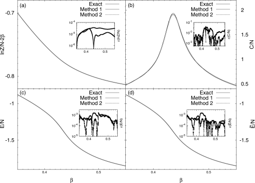
The calculated partition function, average energy and heat capacity are shown in Fig. 2. The thin solid lines and dashed lines are for the method introduced in Sec. 2D (method 1), and that introduced in Appendix B (method 2), respectively. In most cases, both results for the partition function and the average energy coincide with exact results,⁸ see Figs. 2a, 2c, 2d. Even for the heat capacity, which is the second order derivative of the partition function and is harder to compute, the deviations in both cases are small. This indicates that our method is unbiased and it can produce exact thermodynamic quantities asymptotically.

Figure 2.

Thermodynamic quantities as functions of β for the 32×32 Ising model. Results from the method introduced in Sec. 2 are labeled as method 1 (thin solid lines, cross for errors), and those from the method introduced in Appendix B are labeled as method 2 (dashed lines, circles for errors); (a) the partition function, (b) the heat capacity, (c) the average energy, and (d) $\tilde{E}\left(\beta \right)$.

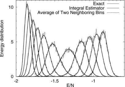
We now show that the correct energy distribution can be reconstructed from Eq. 20. Since the energy levels are discrete and the energy bin size we used was equal to the smallest gap between energy levels, a normalized energy histogram is equivalent to the energy distribution. During simulation, the current potential energy was registered into the histogram every 100 Monte Carlo moves, thus there were roughly 10⁵ samples in the entire histogram. The reconstructed energy distributions at a few representative temperatures are shown in Figure 3. The temperature window for estimating the energy distribution at β was (β−Δβ,β+Δβ) with Δβ=0.02. One can see a good agreement between the integral identity Eq. 20 (the thin solid line), and the exact distribution (thick solid line), which was computed from the exact density of states.⁹ For comparison, distributions constructed by averaging energy distributions of two adjacent bins are shown as dashed lines. It is apparent that the simple average yields more noisy results than the integral identity Eq. 20. The reduced error is due to Eq. 20 being able to access statistics from a much larger temperature window than from two neighboring bins.

Figure 3.

Reconstructed energy distribution at a few temperatures using Eq. 20 with a window size Δβ=0.02 for the 32×32 Ising model. For comparison, we also show the resulting distributions from averaging energy distributions of two adjacent temperature bins, with the bin size δβ=0.0002. The energy distributions constructed from Eq. 20 with a larger window are more precise than those from simple averages of two adjacent bins.

Lennard-Jones system

As the second example, we test the method on an 864-particle Lennard-Jones liquid. In reduced units, the Lennard-Jones potential for a particle pair separated by distance r is

$$u\left(r\right)=4\left(\frac{1}{r^{12}}-\frac{1}{r^6}\right),$$

where the units of energy, mass, and length are 1.0. In the simulation, the density was 0.8; the cutoff was 2.5; and the temperature range was β=(0.48,1.02), corresponding to T=(0.98,2.08). We used Monte Carlo to generate configuration changes. In each step, a random particle was displaced randomly in each of x, y, and z directions according to a uniform distribution in (−0.1,0.1). After a Monte Carlo step, we applied the Langevin equation Eq. 1 with an integration time step Δt=0.0002. The system was simulated for 10⁵ sweeps (a sweep=a step per particle). Coordinates were saved every ten sweeps for data analysis. The overall temperature distribution w(β) was proportional to 1∕β (the choice of optimal w(β) is discussed in Appendix C). The temperature bin for collecting statistics was δβ=0.0005. The window size Δβ for applying the integral identity Eq. 18 was 0.05.

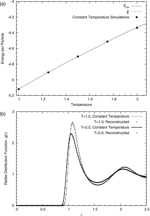
The simulation results for the estimated average energy ⟨E⟩_β and $\tilde{E}\left(\beta \right)$ are shown in Fig. 4a. Due to a small bin size, the difference between the two is invisible. The dots on the figures represent results from independent constant temperature simulations, each of which uses the same amount of simulation time. A good agreement between the two indicates that our method can produce exact thermodynamic quantities for the entire temperature spectrum with less simulation time.

Figure 4.

(a) $\tilde{E}\left(\beta \right)$ of an 864-particle Lennard-Jones system. As a comparison, the values of the average energy from several constant temperature simulations are shown as dots. (b) The reconstructed radial distribution functions of an 864-particle Lennard-Jones system at two selected temperatures T=1.0 and 2.0 are shown as points. As a comparison, the corresponding radial distribution functions from independent constant temperature simulations are shown as lines.

Furthermore, we reconstructed the radial distribution function g(r) at a particular temperature according to Eq. 21. The reconstruction was performed after simulation and was based on the saved coordinates along the trajectory. From Fig. 4b, we see a good agreement between reconstructed g(r)’s and those from constant temperature simulations at two different temperatures β=0.5 and 1.0, or T=2.0 and 1.0, respectively.

APPLICATIONS IN FOLDING SMALL PROTEINS

In this section, we report applications of the method in folding of several small proteins. The method was implemented in a modified GROMACS 4.0.5,¹⁰ using AMBER force field ports¹¹ with TIP3P water model.¹² In all cases, the particle-meshed Ewald method¹³ was used for handling long range electrostatic interaction, and the velocity-rescaling method was used as thermostat.¹⁴ For constraints, we used the SETTLE algorithm for water molecules,¹⁵ and the parallel LINCS algorithm¹⁶ for proteins. Since proteins drastically changed their configurations during simulations, dynamic load balancing was turned on when using domain decomposition.

For configuration-space sampling under a fixed temperature, the canonical ensemble, i.e., the constant (N,V,T) ensemble, was used. A 10 Å cutoff was used for Lennard-Jones interaction, electrostatic interactions and neighboring list. Since the temperature in our method is a variable, the temperature change was realized by scaling the force according to F^′=(β∕β₀)F=(T₀∕T)F, with F^′ and F being the scaled and the original force, respectively. In this way, the scaled potential energy transforms a canonical ensemble at T₀ to another temperature T, for sampling in the configurational space. On the other hand, the thermostat temperature T₀, which controls the kinetic energy, is unaffected and can be maintained at a fixed value T₀=480 K. Three separate thermostats were applied to protein, solvent and ion groups, and the coupling time τ_T for the thermostats was 0.1 ps.

The time step for molecular dynamics was 0.002 ps. The center of mass motion was removed every step. Trajectory snapshots were saved every 2 ps. Since the force and energy calculation was much more time consuming than estimating $\tilde{E}\left(\beta \right)$, we applied the Langevin equation in every molecular dynamics step using an integration step of Δt=10⁻⁴. The parameter C_γ in the adaptive averaging Eq. 23 was 0.1 in all cases.

Trpzip-2

The first system is a 12 amino acid β-hairpin tryptophan zipper, whose Protein Data Bank (PDB) ID code is 1LE1, and its sequence is SWTWENGKWTWK.¹⁷ A unique feature of this short hairpin is that its four tryptophan side chains are locked against each other to stabilize the structure.

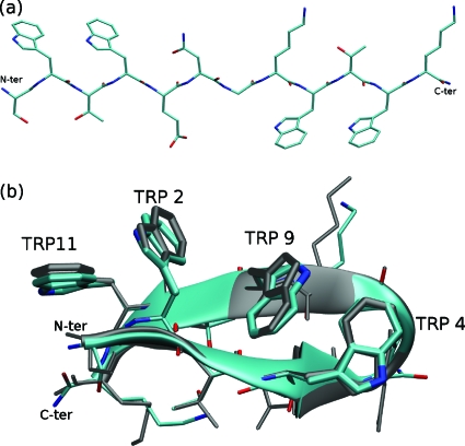
Previously, the system was intensively studied both in explicit solvent¹⁸ and in implicit solvent.^{19, 20} However, de novo folding in explicit solvent from an extended chain, see Fig. 5a, is much more challenging. We used AMBER99SB as the force field, which is a modified version of AMBER99 force field²¹ with updated φ and ψ torsions.²²

Figure 5.

Trpzip2: (a) the initial fully extended conformation, (b) a typical folded structure from trajectory 2. The C_α-RMSD and heavy atom RMSD are 0.25 and 1.08 Å, respectively. Gray: reference structure (PDB ID: 1LE1).

We report four simulation trajectories. All of them reached atomic accuracy within in a time scale of 1 μs. In all the cases, we used a cubic 45×45×45 ų box, filled with 2968 water molecules as well as two Cl⁻ ions. The temperature range was β∊(0.20,0.41), which corresponded to T=293.6–601.9 K temperature range. The grid spacing for Fourier transform was 1.15 Å, and the alpha parameter was 0.3123 Å⁻¹ for the Ewald method. In application of integral identities equations 18, 19, 20, the temperature windows size was 8% of temperature value, e.g., at β=1.0∕(k_B500 K)≈0.241 the temperature window is (β−Δβ,β+Δβ), with Δβ=4%×β≈0.010, which can be translated to T=(480.8,520.8) K. At boundaries, we used the largest possible size that allows a symmetrical window.

A typical folded structure is shown in Fig. 5b, with its root mean square deviations (RMSD) for alpha-carbon (C_α) and heavy atoms being 0.25 and 1.08 Å, respectively. The lowest C_α-RMSD and heavy atom RMSD found in the four trajectories are listed in Table 1, in which we also list the approximate first time of stably reaching the atomically accurate native structure (the criteria were C_α-RMSD<0.5 Å). It is interesting to note that even among structures with lowest RMSDs, tryptophan side chains can still adopt different conformations. For example, in trajectories 1 and 3, we found nativelike structures with one of the tryptophan side chain (TRP9 or TRP4) flipped 180° with respect to the native configuration. This suggests that the free energy change involved in flipping a TRP side chain is small.

Table 1.

Lowest RMSDs and folding time from four independent folding trajectories of trpzip2. Snapshots of reaching the lowest C_α-RMSDs can differ slightly from those of reaching the lowest heavy atom RMSDs.

Traj. ID	Lowest Cα-RMSD (Å)	Lowest heavy atom RMSD (Å)	First time of stably reaching atomic accuracy of the native state (ns)
1	0.20	1.00	20
2	0.25	0.84	520
3	0.20	0.88	530
4	0.25	1.31	1080

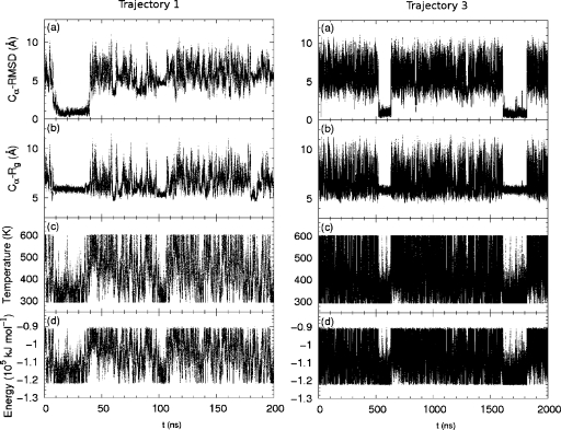
In Fig. 6, C_α-RMSD, radius of gyration, instantaneous temperature, and potential energy along trajectory are shown in (a)–(d), respectively, for the two independent simulations, trajectory 1 and 3. In trajectory 1, the folded state was reached within 20 ns. This suggests the possibility of fast folding. However, in other trajectories, it took longer for the system to reach the native structure. In trajectory 3, upon reaching of the native structure, the system lingered in a state of low-temperature, low-energy state, and small radius of gyration for about 100 ns. This corresponds to the fact that the folded state has a lower energy than the unfolded state and thus occupies a larger fraction in a low temperature Boltzmann distribution. This feature serves as a signature of the system reaching a native structure, and can be useful in folding prediction where the native structure is unknown.

Figure 6.

Trpzip2: quantities along two independent simulation trajectories. Left: the first 200 ns of a fast-folding trajectory (trajectory 1). Right: 2 μs of trajectory 3. Panels from top to bottom: (a) C_α-RMSD from native structure, (b) C_α radius of gyration, (c) temperature, and (d) potential energy.

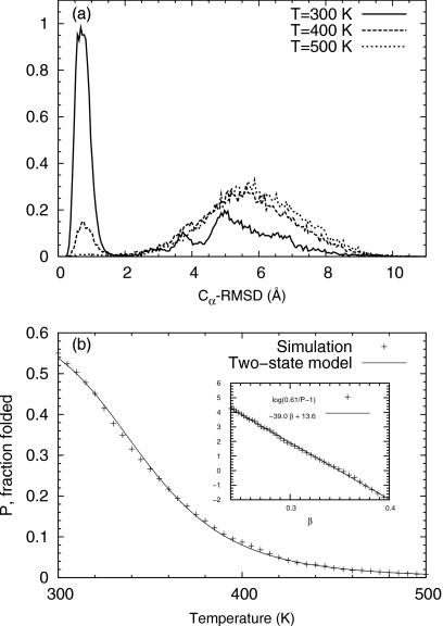
Figure 7a shows the distribution along the C_α-RMSD at three different temperatures calculated from trajectory 3. The distribution demonstrates two well-separated peaks, corresponding to roughly defined folded and the unfolded states, respectively. The average C_α-RMSD from the native structure is roughly 0.8 and 5.5 Å for folded and unfolded states, respectively. As the temperature increases, the first peak gradually diminishes, whereas the second peak dominates.

Figure 7.

Trpzip2: (a) distribution along the RMSD from the native structure at three temperatures 300, 400, and 500 K, calculated from trajectory 3 and (b) fraction P of the folded state vs the temperature. Inset: linear fitting of log(P₀∕P−1) vs β according to the two-state model.

The folding temperature can be computed by assuming a two-state model of folding. The folding fraction P was first calculated as the fraction of configurations with C_α-RMSD less 2.0 Å at different temperatures. The curve P(β) as a function of temperature β was then fitted against a two-state model in the range β∊(0.24,0.4), equivalentlyT∊(300.9 K,501.5 K),

$$P=\frac{P_0}{1+\text{exp}\left[\Delta E\left({\beta }_{\text{m}}-\beta \right)\right]},$$ (24)

where the values of the three parameters were determined as P₀=0.61, ΔE=38.96 kJ mol⁻¹, and β_m=0.350 kJ⁻¹ mol by regression, see Fig. 7b. Here, ΔE is the energy difference between the folded state and the unfolded state; β_m is the melting temperature. In the simplest two-state model, the folding fraction increases monotonically to unity as the temperature decreases to zero. Here, the maximal fraction was changed from 1.0 to an adjustable parameter P₀, which helped fitting the calculated P(β) to the two-state model. Physically, such a modification implies the existence of many configurations with energy similar to that the native one but with different structures in our simulation trajectory.

If the volume change during folding is ignored, the enthalpy change between the folded state and the unfolded state is roughly equal to the energy change ΔH≈39.0 kJ mol⁻¹. The entropy difference of the folded and unfolded states is ΔS=β_mΔE=113 J mol⁻¹. These values are relatively small compared with the experimental values ΔH^exp=70.2 kJ mol⁻¹, ΔS^exp=203.3 J mol⁻¹.¹⁷ However, the estimated folding temperature from our calculation 344 K is close to the experimental result 345 K.¹⁷ From trajectory 3, which yields the highest folding fraction at 300 K among four trajectories, the fraction of folded states at 300 K is roughly 55%, which still differs significantly from the experimental value 91%.¹⁷ For the other three trajectories, the calculated fractions are even smaller. The difference between our calculation and experiments were likely due to insufficient sampling and∕or force field inaccuracy.

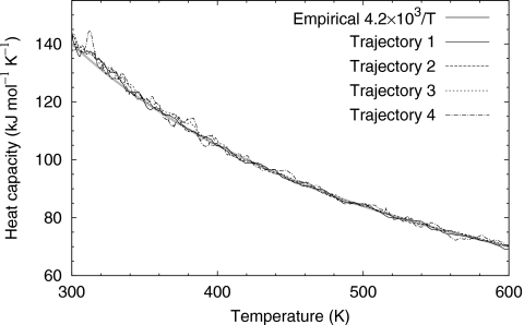
Figure 8 shows the heat capacity versus temperature from Eq. 19. The difference between three independent trajectories was small, suggesting thermodynamic properties of the entire system, protein and water, reaching convergence. It is interesting that in our simulation, the heat capacity is not a constant, but inversely proportional to the temperature as C_V≈4.2×10³∕T kJ mol⁻¹ K⁻¹.

Figure 8.

Trpzip2: the heat capacity, computed from four independent trajectories. Bold solid line: empirical formula C_V≈4.2×10³∕T.

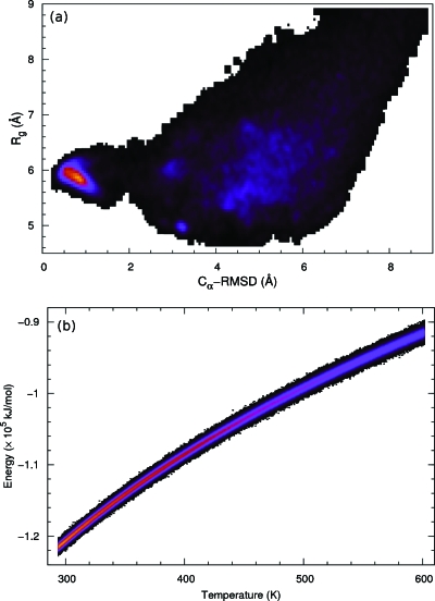
Figure 9a shows the joint distribution of the radius of gyration R_g (calculated from C_α atoms) and the C_α-RMSD. Generally the two measures are positively correlated. However, the smallest radius of gyration does not occur at the native structure for the hairpin, whose R_g is roughly around 5.8 Å. A non-native structure, on the other hand, had a smaller R_g around 4.9 Å, but a larger RMSD around 3 Å. Figure 9b shows the joint distribution of temperature and energy. A typical temperature fluctuation is only around 5 K, which is roughly the magnitude of temperature gap in other tempering methods based on a discrete temperature, such as replica exchange. On the other hand, the temperature window size used in our simulation was much larger. This suggests that our method could more efficiently use statistics to facilitate the temperature-space random walk.

Figure 9.

Trpzip2: joint distributions of (a) the radius of gyration vs C_α-RMSD and (b) the potential energy vs temperature. A brighter color represents a higher population density.

Trp-cage

The second application is a 20 amino acid alpha helical protein, tryptophan cage (trp-cage).²³ The PDB code is 1L2Y, and the amino acid sequence is NLYIQWLKDGGPSSGRPPPS. The system was extensively studied by experiments^{23, 24} as well as by various sampling techniques, either in explicit solvent^{25, 26} or in implicit solvent.^{20, 27} We again used AMBER99SB as the force field.²²

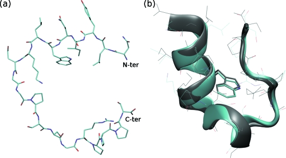
We simulated the system in a cubic 46×46×46 ų box, filled with 3161 water molecules and two Cl⁻ ions. The grid spacing for Fourier transform was 1.19 Å, and the alpha parameter was 0.3123 Å⁻¹. The initial structure was an open chain see Fig. 10a, which was constructed by bending a fully extended chain to fit into the box.

Figure 10.

Trp-cage: (a) the initial fully extended structure, (b) a typical folded structure. The C_α-RMSD and the all heavy atom RMSD are 0.44 and 1.54 Å, respectively. Gray: reference structure (PDB ID: 1L2Y).

We report three independent 1 μs simulation trajectories. The temperature range for trajectory 1 was β∊(0.24,0.41), or T∊(293.6 K,501.5 K). In trajectories 2 and 3, we used a larger temperature range β∊(0.20,0.41), which covered a 293.6 K∼601.9 K temperature range. The temperature bin size δβ was 0.0005, 0.0005, and 0.0002 respectively. In applying integral estimators, the temperature windows size was 10%, 10%, and 8% of temperature value for trajectories 1, 2, and 3, respectively. In all cases, we used the alternative estimator introduced in Appendix B.

All three simulations independently reached atomically accurate native configurations. A typical folded structure in trajectory 1 is shown in Fig. 10b. The C_α-RMSDs from the three trajectories were 0.43, 0.48, and 0.44 Å, respectively. The average C_α-RMSD for the native structure was around 0.8 Å. The lowest RMSDs for all heavy atoms were 1.34, 1.47, and 1.46 Å, respectively.

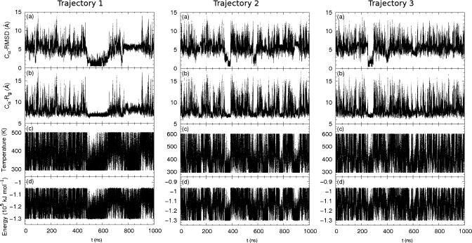
The C_α-RMSD, radius of gyration, instantaneous temperature, and potential energy along trajectory are shown in panels (a)–(d), respectively, of Fig. 11, for the three independent simulations. In each trajectory, there were two folding events reaching an atomic accuracy, e.g., for trajectory 2, the native structure was reached at 350 and 560 ns. As in the trpzip2 case, the system stayed around a low-temperature and low-energy state for 30–100 ns upon reaching the native state. For the folding speed, it appears that simulations 2 and 3, which used a higher roof temperature T_max=600 K, tended to reach the native state sooner than simulation 1, whose roof temperature T_max=500 K was lower. However, in simulation 1, the system was able to stay in the native states longer and performed a more detailed sampling at the low temperature end.

Figure 11.

Trp-cage: three independent trajectories (a) C_α-RMSD from native structure, (b) C_α radius of gyration, (c) temperature, and (d) potential energy.

Trajectory 1 yielded the largest fraction of the folded state at 300 K, 19%, which is still much lower than experiment value, 70%.^{23, 28} By fitting the folding fraction, computed from the fraction of states with C_α-RMSD less than 2.2 Å cutoff, to the two-state formula Eq. 24, the parameters are P₀=0.50, ΔE=21.1 kJ mol⁻¹, and β_m=0.367 kJ⁻¹ mol. The enthalpy change is thus ΔH≈21 kJ mol⁻¹, which is relatively small compared with the experimental values ΔH^exp=56.2 kJ mol⁻¹.²⁸ The estimated folding temperature from our calculation is 328 K, which is slightly higher than the experimental result 315 K.²⁸

Villin headpiece

Our last application was the villin headpiece, a 36 residue alpha-helical protein HP36. The PDB ID is 1VII, and the amino acid sequence is MLSDEDFKAVFGMTRSAFANLPLWKQQNLKKEKGLF. This system was the first protein partially folded in explicit solvent.²⁹ Recently, a high resolution x-ray structure of slightly modified protein HP35, PDB ID 1YRF, was published.³⁰ The sequence of HP35 is LSDEDFKAVFGMTRSAFANLPLWKQQHLKKEKGLF, in which the N-terminal methionine (MET) of the original sequence was chopped off and the 28th residue, an asparagine, was replaced by a hisidine. Both sequences were studied in literature, both by simulations,^{31, 32, 33, 34} and in experiments.^{35, 36}

However, there is a significant difference between the NMR structure of HP36 and the x-ray structure of HP35, about 1.62 Å difference in terms of C_α-RMSD. Further, while molecular dynamics simulations on HP35 reached an atomic accuracy in implicit solvent³² as well as in explicit solvent,³⁴ simulations on HP36, especially in explicit solvent, yielded relatively poorer results. The difference between the two structures could be due to (1) the intrinsic difference between HP35 and HP36 or (2) differences in the two experimental techniques, NMR versus x ray.³⁰

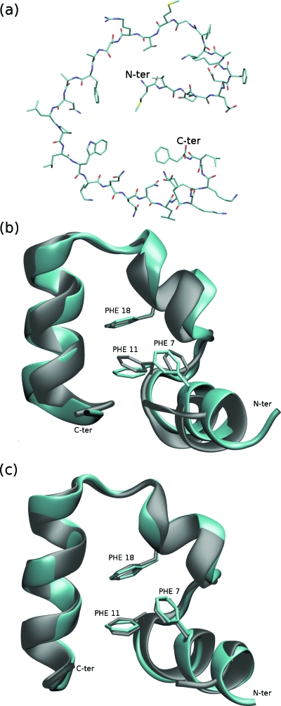
In this simulation, we used AMBER03 (Ref. ³⁷) as the force field, which was previously used to fold HP35 to an atomic accuracy in implicit solvent.³² Another reason of choosing AMBER03 instead of AMBER99SB was that the latter force field might slightly disfavor helical conformations.³⁸ To reduce simulation size, we used a dodecahedron simulation box with edge length being 24.1 Å to accommodate the protein as well as 3343 water molecules, and two Cl⁻ ions. The volume of the box was 53.3×53.3×37.6 ų=1.069×10⁵ ų. The initial conformation of the protein was a fully extended chain, which was bent from a linear chain to fit into the box, see Fig. 12a. The grid spacing for Fourier transform was 1.19 Å and the alpha parameter was 0.3123 Å⁻¹.

Figure 12.

Villin headpiece: (a) the initial fully extended structure, (b) a typical folded structure compared with an NMR reference structure (gray, PDB ID: 1VII, C_α-RMSD: 1.15 Å), (c) a typical folded structure compared with an x-ray structure (gray, PDB ID: 1YRF, C_α-RMSD: 0.47 Å), and the N-terminal is not shown due to the sequence difference.

We report two independent simulation trajectories, each of 2 μs. The temperature range for trajectory 1 was β∊(0.18,0.41), or T∊(293.6 K,668.7 K); that for trajectory 2 was β∊(0.20,0.41), or T∊(293.6 K,601.9 K). The temperature bin size was 0.0002 in both cases. The integral estimator introduced in the Sec. 2 was used, and the temperature windows size was 8% of current temperature value.

The alpha-carbon root mean square deviation can be calculated from the NMR structure as well as the x-ray structure. In both cases, the N-terminal MET and leucine (LEU) as well as the C-terminal phenylalanine (PHE) are not included in our calculation.³² Due to the flexibility of the C-terminal and the N-terminal helix, we also calculate the C_α-RMSD for residues 9–32 of HP36 as in the literature,^{29, 31} denoted as RMSD_core here. Note, in terms of C_α-RMSD_core, the NMR reference structure differs from the x-ray reference structure by 0.87 Å.

The lowest C_α-RMSDs reached in the two simulation trajectories are listed in Table 2. The lowest C_α-RMSD_core from the NMR structure are 0.72 and 0.73 Å, for the two trajectories, respectively. These figures are smaller than those from a previous study, in which the lowest RMSD_core was around 1.5 Å.³¹ In both trajectories, the best folded structures are more similar to the x-ray structure than to the NMR structure. The average C_α-RMSD and C_α-RMSD_core from the NMR structure are 1.30 and 1.95 Å, respectively. In comparison, the two figures drop to 0.90 and 1.10 Å if the reference is switched to the x-ray structure.

Table 2.

Lowest RMSDs in angstrom reached in two folding trajectories of villin headpiece. Snapshots of reaching the lowest C_α-RMSDs can differ slightly from those of reaching the lowest heavy atom RMSDs. The reference structures (either the NMR or x-ray structure) are denoted in parentheses.

Traj. ID	RMSDcore (NMR)	RMSD (NMR)	RMSDcore (x ray)	RMSD (x ray)	First time of reaching atomic accuracy of the native state (ns)
1	0.72	1.32	0.30	0.42	310
2	0.73	0.99	0.30	0.40	26

Table 2 also lists the first time for reaching the native structure. In both trajectories, the time (310 ns for trajectory 1 and 26 ns for trajectory 2) is significantly shorter than those in a very recent study (where the folding occurs in 5–6 μs).³⁴

In Figs. 12b, 12c, we show the superposition of typical folded structures to the NMR reference structure and the x-ray reference structure, respectively, from simulation 1. Although generally deviations from the native structures are small, the position of the N-terminal helix differs appreciably from the NMR native structure [notice the difference in position of PHE 7 and PHE 11 in Fig. 12b], whereas the difference is much smaller compared with the x-ray structure [PHE 7 and PHE 11 of the two structures are superimposable in Fig. 12c].

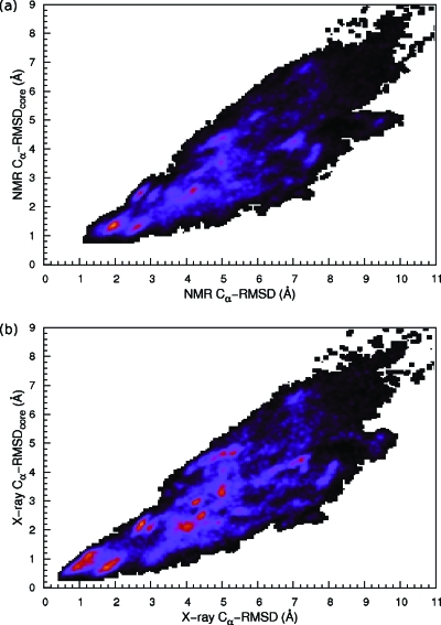
Figures 13a, 13b show the C_α-RMSD_core (the stable region residues 9–32) versus the C_α-RMSD (entire chain) for the NMR and x-ray reference structures, respectively. It is clear that the best folded structures have larger deviations from the NMR structure than from the x-ray structure. Moreover, the C_α-RMSD_core is less consistent with the C_α-RMSD with respect to the NMR structure than to the x-ray structure, which can be a result of the extremely flexible N-terminal helix. In general, we found that the folded structures in our simulation are closer to the x-ray structure. In both case, we observe many metastable states around the native state, demonstrating an extremely rugged energy landscape.

Figure 13.

Villin headpiece: joint distributions of (a) C_α-RMSD and C_α-RMSD_core (from residues 9∼32) using the NMR structure as the reference and (b) C_α-RMSD and C_α-RMSD_core, using the x-ray structure as the reference. Statistics from the two trajectories were combined.

The folding fraction, computed according to C_α-RMSD from the x-ray structure and using 3.0 Å as cutoff, was fitted against Eq. 24, and yielded P₀=0.21, ΔE=20.9 kJ mol⁻¹, and β_m=0.349 kJ⁻¹ mol. Assuming that the volume change during folding is negligible, we estimate the enthalpy change ΔH=21 kJ mol⁻¹, and the folding temperature T_m=345 K. Although the folding temperature agrees well with the experimental value 342 K, the folding enthalpy is relatively small compared to ΔH^exp=113 kJ mol⁻¹.³⁵

CONCLUDING DISCUSSIONS

In conclusion, we presented a single-copy enhanced sampling method for studying large complex biological systems. The method was validated in an Ising model as well as in a Lennard-Jones fluid, and was successfully applied to folding of three small proteins, trpzip2, trp-cage, and villin headpiece, in explicit solvent. In all three protein cases, we reversibly reached atomic accuracy of the native structures within a microsecond. Since our method is based on a single trajectory, it is computationally less demanding to reach a long time scale than tempering methods based on multiple copies, such as the replica exchange method.

In terms of sampling efficiency, in addition to the advantage from using a continuous temperature generalize ensemble, which eases the issue of low temperature-transition rate in large complex systems,² a major improvement in this work is the employment of integral identity that efficiently estimates the average energy $\tilde{E}\left(\beta \right)$ for the temperature space random walk. The integral identity draws estimates from a large temperature window instead of from a single bin to improve statistics. This strategy makes the method more robust and applicable to large and complex systems.

Additionally, the adaptive averaging scheme used for refreshing statistics can effectively boost the temperature space random walk in early stages, when the damping magnitude γ still differs significantly from unit. It could account for several fast folding (<50 ns) events we observed. However, in later stages of simulations, the boosting effect gradually weakens as the damping magnitude γ is switched toward 1.0 [see Eq. 23] to achieve an asymptotic convergence.

In folding applications, the calculated values for the folding enthalpy and folding temperature still showed discrepancies from experimental results. This was possibly due to errors in the force fields^{26, 34} as well as limited simulation time. These factors might lead to overpopulation of non-native conformations at room temperature. This observation is in line with a very recent long time replica exchange simulation on trp-cage with an aggregated 40×1 μs, which also revealed discrepancy between experimental and simulation results.²⁶ Even in the presence of enhanced sampling, one would desire to perform much longer simulations to allow much more folding events to atomic accuracy. In this way, one can more accurately examine population ratios of the native conformation to various folding intermediate and non-native conformations.

APPENDIX A: FOKKER–PLANCK EQUATION AND STATIONARY DISTRIBUTION

Though the temperature distribution of the generalized ensemble is uniquely specified by Eq. 8, various Langevin equations exist for sampling the distribution, e.g., both Eq. 1 and the one used in the previous study² correctly populate the distribution.

Before applying a Langevin equation, one needs to find a proper “potential” V(β) for the temperature to guide its diffusion. The potential is the negative logarithm of the temperature distribution

$$V\left(\beta \right)\equiv -\text{ln}p\left(\beta ,X\right).$$

The negative derivative of the potential naturally serves as the force of driving the temperature space random walk. According to Eq. 8, we have

$$\frac{\partial V\left(\beta \right)}{\partial \beta }=\frac{\partial \left[-\text{ln}p\left(\beta ,X\right)\right]}{\partial \beta }=E+\frac{\partial \text{\hspace{0.17em}ln}\tilde{Z}\left(\beta \right)}{\partial \beta }-\frac{\partial \text{\hspace{0.17em}ln}w\left(\beta \right)}{\partial \beta }.$$

Equation 1 is now simplified as

$$\frac{d\left(1∕\beta \right)}{dt}=\frac{dV\left(\beta \right)}{d\beta }+\frac{\sqrt{2}}{\beta }\xi .$$ (A1)

To show that Eq. A1 is correct, we introduce a new variable τ=1∕β=k_BT and write down the Fokker–Planck equation that governs the distribution of τ or ρ(τ)

$$\frac{\partial \rho \left(\tau \right)}{\partial t}=\frac{\partial }{\partial \tau }\left[-\frac{\partial V}{\partial \beta }\rho \left(\tau \right)\right]+\frac{{\partial }^2}{\partial {\tau }^2}\left[{\tau }^2\rho \left(\tau \right)\right]=\frac{\partial }{\partial \tau }\left[\rho \left(\tau \right){\tau }^2\frac{\partial V}{\partial \tau }\right]+\frac{{\partial }^2}{\partial {\tau }^2}\left[{\tau }^2\rho \left(\tau \right)\right],$$ (A2)

where we have used −τ²(∂∕∂τ)=∂∕∂β. A stationary solution of Eq. A2 can be found by solving the following equation:

$$-\left[{\tau }^2\rho \left(\tau \right)\right]\frac{\partial V}{\partial \tau }=\frac{\partial }{\partial \tau }\left[{\tau }^2\rho \left(\tau \right)\right],$$

whose solution is readily obtained,

$${\tau }^2\rho \left(\tau \right)\sim \text{exp}\left(-V\right)=p\left(\beta ,X\right).$$

Finally, we translate the distribution of τ back to that of β according to the probability invariance ρ(β)dβ=ρ(τ)dτ,

$$\rho \left(\beta \right)d\beta =\rho \left(\tau \right)d\tau =\rho \left(\tau \right)d\beta ∕{\beta }^2=\rho \left(\tau \right){\tau }^{2}d\beta .$$

We thus conclude that ρ(β)=τ²ρ(τ)=p(β,X), which proves that Eq. 8 is the stationary solution of the Fokker–Planck equation.

APPENDIX B: ALTERNATIVE FITTING BASED ESTIMATOR

Here we introduce an alternative estimator for $\tilde{E}\left(\beta \right)$ based on linear extrapolation. First, we generalize Eq. 15 to the following. For any function

$$f\left(\beta \right)={⟨E⟩}_{\beta }+k\left({\overline{\beta }}_i-\beta \right),$$ (B1)

where ${\overline{\beta }}_i=\left({\beta }_i+{\beta }_{i+1}\right)∕2$ and k is an arbitrary constant, we have

$${\tilde{E}}_i=\frac{1}{\Delta {\beta }_i}{\int }_{{\beta }_i}^{{\beta }_{i+1}}d\beta {⟨E⟩}_{\beta }=\frac{1}{\Delta {\beta }_i}{\int }_{{\beta }_i}^{{\beta }_{i+1}}d\beta f\left(\beta \right)={\int }_{{\beta }_{-}}^{{\beta }_{+}}d\beta {\varphi }_s^{\prime }\left(\beta \right)f\left(\beta \right)+{\int }_{{\beta }_{-}}^{{\beta }_{+}}d\beta \varphi \left(\beta \right)f^{\prime }\left(\beta \right),$$ (B2)

where on the second line, the linear term in Eq. B1 vanishes after the integration. Equation 15 can be considered as a special case for k=0.

Equations B1, B2 allow a properly extrapolation for the average energy ⟨E⟩_β from β to ${\overline{\beta }}_i$ before applying the integral identity, or the temperature averaging. If we assume that ⟨E⟩_β is roughly linear function of β in the window (β₋,β₊), the slope k of ⟨E⟩_β versus β can be obtained from linear regression as

$$k={⟨\Delta \beta \Delta E⟩}_{+}∕{⟨\Delta {\beta }^2⟩}_{+},$$ (B3)

where the angular bracket ⟨⋯⟩₊ denotes a temperature average over (β₋,β₊).

The advantage of using Eq. B2 is that it reduces the magnitude of the second integral and thus makes the estimator more robust. If the relation of ⟨E⟩_β and β is perfectly linear, f^′(β)=∂⟨E⟩_β∕∂β−k vanishes everywhere, and thus the second integral yields zero.

In practice, we use a ϕ(β) parameterized with a₊=a₋=1∕2, and restrain the magnitude of the second integral within the average energy fluctuation $\sqrt{{⟨\Delta E^2⟩}_{+}}$ in the window to ensure stability of the estimator.

The estimator introduced here can be thought as a first-order generalization of Eq. 15, and thus allows a large temperature window or application to larger systems. Besides, one can also apply additional constraints to the derivative to improve the accuracy and stability of the estimator. For example, in our case of estimating the average energy, the derivative k corresponds to the negative energy fluctuation as ∂⟨E⟩_β∕∂β=−⟨ΔE²⟩_β=−k_BT²C_V (where C_V is the heat capacity), and its value can be restrained within a certain range. In the systems tested in this work, however, it did not produce significantly different estimates from the one introduced in the Sec. 2D.

APPENDIX C: CHOICE OF THE TEMPERATURE DISTRIBUTION ω(β)

Here, we discuss the optimal choice of w(β). For molecular systems, we invariably use w(β)≈p(β)∼1∕β basing on the following reason. The overall energy distribution p(E) of the generalized ensemble is a superposition of energy distributions of canonical ensembles from different temperatures. To ensure a fixed degree of overlap, the height of p(E) only needs to match that of a canonical distribution at β, whose average energy ⟨E(β)⟩ is roughly equal to E. The average height of a canonical ensemble is inversely proportional to its width $\sqrt{{⟨\Delta E^2⟩}_{\beta }}$, and thus,

$$p\left(E\right)dE\propto \frac{dE}{\sqrt{{⟨\Delta E^2⟩}_{\beta }}}.$$

To translate the energy distribution to the temperature space, we change variable from E to β. According to the probability invariance p(E)dE=p(β)dβ, and |dE∕dβ|=⟨ΔE²⟩_β, we have

$$w\left(\beta \right)\propto \frac{\left|dE∕d\beta \right|}{\sqrt{{⟨\Delta E^2⟩}_{\beta }}}\propto \sqrt{{⟨\Delta E^2⟩}_{\beta }}\propto \frac{\sqrt{C}}{\beta },$$

In the last step, we have used fact that k_Bβ²⟨ΔE²⟩_β=C, where C is the heat capacity.

For a Lennard-Jones-like system, the heat capacity C is roughly a constant, accordingly the optimal w(β) is proportional to 1∕β. On the other hand, our protein simulations show that the heat capacity of the entire system, water and protein, roughly follows C∝β, see Fig. 8. According to this observation, the optimal w(β) should be proportional to $1∕\sqrt{\beta }$. However, in our simulations, we still used 1∕β as w(β), this setup slightly biases the ensemble toward the high temperature end in order to encourage a faster motion at higher temperature and to help overcome broken ergodicity at lower temperature.

APPENDIX D: INTEGRAL IDENTITY FOR A NON-NEGATIVE QUANTITY

For a histogram-like quantity, regular integral identities such as Eq. 15 should be modified to ensure the output is non-negative. Here, we briefly sketch a technique for this purpose (a more detailed and general treatment is presented elsewhere⁶).

Suppose h(β) is a non-negative quantity, and we are interested in estimating its value at a particular temperature β^*. Instead of applying an integral identity to h(β) itself, we introduce a smooth modulating function f(β), with f(β^*)=1, and apply the identity to the product h(β)f(β),

$$h\left({\beta }^{*}\right)=h\left({\beta }^{*}\right)f\left({\beta }^{*}\right)={\int }_{{\beta }_{-}}^{{\beta }_{+}}\left[h\left(\beta \right)f\left(\beta \right)\right]{\varphi }^{\prime }\left(\beta \right)d\beta +{\int }_{{\beta }_{-}}^{{\beta }_{+}}{\left[h\left(\beta \right)f\left(\beta \right)\right]}^{\prime }\varphi \left(\beta \right)d\beta .$$ (D1)

If we choose

$$f\left(\beta \right)=\text{exp}\left(-{\int }_{{\beta }^{*}}^{\beta }{\left[\text{ln}h\left({\beta }^{\prime }\right)\right]}^{\prime }d{\beta }^{\prime }\right),$$ (D2)

the second term on the right hand side of Eq. D1 vanishes because [h(β)f(β)^]′=0 everywhere. Thus, the estimated value is always non-negative given that ϕ^′(β)≥0. ϕ^′(β) satisfies the normalization condition ${\int }_{{\beta }_{-}}^{{\beta }_{+}}{\varphi }^{\prime }\left(\beta \right)d\beta =1$, and should be proportional to w(β)∕f(β) to minimize the error. Thus, the general expression for h(β^*) is

$$h\left({\beta }^{*}\right)=\frac{{\int }_{{\beta }_{-}}^{{\beta }_{+}}w\left(\beta \right)h\left(\beta \right)d\beta }{{\int }_{{\beta }_{-}}^{{\beta }_{+}}w\left(\beta \right)\text{exp}\left({\int }_{{\beta }^{*}}^{\beta }{\left[\text{ln}h\left({\beta }^{\prime }\right)\right]}^{\prime }d{\beta }^{\prime }\right)d\beta }.$$ (D3)

In the case of energy histogram, h(β) can defined as an integral of the canonical energy distribution at β over a small energy bin ΔE,

$$h\left(\beta \right)={\int }_E^{E+\Delta E}\frac{g\left(E^{\prime }\right)\text{exp}\left(-\beta E^{\prime }\right)}{Z\left(\beta \right)}d{E}^{\prime }=\left({\int }_E^{E+\Delta E}{p}_{\beta }\left(E^{\prime }\right)d{E}^{\prime }\right)∕w\left(\beta \right),$$

where g(E^′) is the density of states; on the second line, we have used the distribution function of the generalized ensemble p_β(E^′)=w(β)g(E^′)exp(−βE^′)∕Z(β).

It can be straightforwardly verified that

$${\left[\text{ln}h\left(\beta \right)\right]}^{\prime }=-{\left[\text{ln}Z\left(\beta \right)\right]}^{\prime }-\frac{{\int }_E^{E+\Delta E}{E}^{\prime }g\left(E^{\prime }\right)\text{exp}\left(-\beta E^{\prime }\right)d{E}^{\prime }}{{\int }_E^{E+\Delta E}g\left(E^{\prime }\right)\text{exp}\left(-\beta E^{\prime }\right)d{E}^{\prime }}\approx -{\left[\text{ln}Z\left(\beta \right)\right]}^{\prime }-\left(E+\Delta E∕2\right),$$

where on the last line, we assumed that the energy bin size ΔE is sufficiently small such that a typical energy distribution does not vary drastically within a bin. Practically, it only requires the bin size ΔE to be much smaller than the fluctuation (or width) of a typical energy distribution. We finally reached

$$h\left({\beta }^{*}\right)\approx \frac{{\int }_{{\beta }_{-}}^{{\beta }_{+}}{\int }_E^{E+\Delta E}p\left(\beta ,E^{\prime }\right)d{E}^{\prime }d\beta }{{\int }_{{\beta }_{-}}^{{\beta }_{+}}w\left(\beta \right)Z\left({\beta }^{*}\right)∕Z\left(\beta \right)\text{exp}\left[-\left(\beta -{\beta }^{*}\right)\left(E+\Delta E∕2\right)\right]d\beta }.$$

By substituting $\tilde{Z}\left(\beta \right)$ for Z(β), we recover Eq. 20.

References

- Lyubartsev A. P., Martsinovski A. A., Shevkunov S. V., and Vorontsovvelyaminov P. N., J. Chem. Phys. 96, 1776 (1992) 10.1063/1.462133 [DOI] [Google Scholar]; Marinari E. and Parisi G., Europhys. Lett. 19, 451 (1992) 10.1209/0295-5075/19/6/002 [DOI] [Google Scholar]; Zhang C. and Ma J., Phys. Rev. E 76, 036708 (2007) 10.1103/PhysRevE.76.036708 [DOI] [PMC free article] [PubMed] [Google Scholar]; Li H., Fajer M., and Yang W., J. Chem. Phys. 126, 024106 (2007) 10.1063/1.2424700 [DOI] [PubMed] [Google Scholar]; Gao Y. Q., J. Chem. Phys. 128, 064105 (2008); 10.1063/1.2825614 [DOI] [PubMed] [Google Scholar]; Kim J., Straub J. E., and Keyes T., Phys. Rev. Lett. 97, 050601 (2006). 10.1003/PhysRevLett.97.050601 [DOI] [PubMed] [Google Scholar]
- Zhang C. and Ma J., J. Chem. Phys. 130, 194112 (2009). 10.1063/1.3139192 [DOI] [PMC free article] [PubMed] [Google Scholar]
- Geyer C. J., Proceedings of the 23rd Symposium on the Interface (American Statistical Association, New York, 1991); Hansmann U. H. E., Chem. Phys. Lett. 281, 140 (1997) 10.1016/S0009-2614(97)01198-6 [DOI] [Google Scholar]; Hukushima K. and Nemoto K., J. Phys. Soc. Jpn. 65, 1604 (1996) 10.1143/JPSJ.65.1604 [DOI] [Google Scholar]; Swendsen R. H. and Wang J. S., Phys. Rev. Lett. 57, 2607 (1986); 10.1103/PhysRevLett.57.2607 [DOI] [PubMed] [Google Scholar]; Kim J., Straub J. E., and Keyes T., J. Chem. Phys. 132, 224107 (2010). 10.1063/1.3432176 [DOI] [PMC free article] [PubMed] [Google Scholar]
- Darve E. and Pohorille A., J. Chem. Phys. 115, 9169 (2001) 10.1063/1.1410978 [DOI] [Google Scholar]; Fasnacht M., Swendsen R. H., and Rosenberg J. M., Phys. Rev. E 69, 056704 (2004). 10.1103/PhysRevE.69.056704 [DOI] [PubMed] [Google Scholar]
- Adib A. B. and Jarzynski C., J. Chem. Phys. 122, 014114 (2005). 10.1063/1.1829631 [DOI] [PubMed] [Google Scholar]
- Zhang C. and Ma J., arXiv:1005.0170 (2010).
- Ferrenberg A. M. and Swendsen R. H., Phys. Rev. Lett. 61, 2635 (1988) 10.1103/PhysRevLett.61.2635 [DOI] [PubMed] [Google Scholar]; Ferrenberg A. M. and Swendsen R. H., Phys. Rev. Lett. 63, 1195 (1989). 10.1103/PhysRevLett.63.1195 [DOI] [PubMed] [Google Scholar]
- Ferdinand A. E. and Fisher M. E., Phys. Rev. 185, 832 (1969). 10.1103/PhysRev.185.832 [DOI] [Google Scholar]
- Beale P. D., Phys. Rev. Lett. 76, 78 (1996). 10.1103/PhysRevLett.76.78 [DOI] [PubMed] [Google Scholar]
- van der Spoel D., Lindahl E., Hess B., Groenhof G., Mark A. E., and Berendsen H. J., J. Comput. Chem. 26, 1701 (2005) 10.1002/jcc.20291 [DOI] [PubMed] [Google Scholar]; Hess B., Kutzner C., van der Spoel D., and Lindahl E., J. Chem. Theory Comput. 4, 435 (2008) 10.1021/ct700301q [DOI] [PubMed] [Google Scholar]; Lindahl E., Hess B., and van der Spoel D., J. Mol. Model. 7, 306 (2001) [Google Scholar]; Berendsen H. J. C. and van der Spoel D., Comput. Phys. Commun. 91, 43 (1995). 10.1016/0010-4655(95)00042-E [DOI] [Google Scholar]
- Sorin E. J. and Pande V. S., Biophys. J. 88, 2472 (2005). 10.1529/biophysj.104.051938 [DOI] [PMC free article] [PubMed] [Google Scholar]
- Jorgensen J. C. W. L., Madura J. D., Impey R. W., and Klein M. L., J. Chem. Phys. 79, 926 (1983). 10.1063/1.445869 [DOI] [Google Scholar]
- Essman U., Perera L., Berkowitz M. L., Darden T., Lee H., and Pedersen L. G., J. Chem. Phys. 103, 8577 (1995). 10.1063/1.470117 [DOI] [Google Scholar]
- Bussi G., Donadio D., and Parrinello M., J. Chem. Phys. 126, 014101 (2007). 10.1063/1.2408420 [DOI] [PubMed] [Google Scholar]
- Miyamoto S. and Kollman P. A., J. Comput. Chem. 13, 952 (1992). 10.1002/jcc.540130805 [DOI] [Google Scholar]
- Hess B., J. Chem. Theory Comput. 4, 116 (2008). 10.1021/ct700200b [DOI] [PubMed] [Google Scholar]
- Cochran A. G., Skelton N. J., and Starovasnik M. A., Proc. Natl. Acad. Sci. U.S.A. 98, 5578 (2001). 10.1073/pnas.091100898 [DOI] [PMC free article] [PubMed] [Google Scholar]
- Zhang J., Qin M., and Wang W., Proteins 62, 672 (2006) 10.1002/prot.20813 [DOI] [PubMed] [Google Scholar]; Pitera J. W., Haque I., and Swope W. C., J. Chem. Phys. 124, 141102 (2006). 10.1063/1.2190226 [DOI] [PubMed] [Google Scholar]
- Yang L., Shao Q., and Gao Y. Q., J. Phys. Chem. B 113, 803 (2009) 10.1021/jp803160f [DOI] [PubMed] [Google Scholar]; Snow C. D., Qiu L., Du D., Gai F., Hagen S. J., and Pande V. S., Proc. Natl. Acad. Sci. U.S.A. 101, 4077 (2004) 10.1073/pnas.0305260101 [DOI] [PMC free article] [PubMed] [Google Scholar]; Roitberg A. E., Okur A., and Simmerling C., J. Phys. Chem. B 111, 2415 (2007) 10.1021/jp068335b [DOI] [PMC free article] [PubMed] [Google Scholar]; Chen C. and Xiao Y., Bioinformatics 24, 659 (2008) 10.1093/bioinformatics/btn029 [DOI] [PubMed] [Google Scholar]; Yang W. Y., Pitera J. W., Swope W. C., and Gruebele M., J. Mol. Biol. 336, 241 (2004). 10.1016/j.jmb.2003.11.033 [DOI] [PubMed] [Google Scholar]
- Ulmschneider J. P., Ulmschneider M. B., and Di Nola A., J. Phys. Chem. B 110, 16733 (2006). 10.1021/jp061619b [DOI] [PubMed] [Google Scholar]
- Wang J., Cieplak P., and Kollman P. A., J. Comput. Chem. 21, 1049 (2000). 10.1002/1096-987X(200009)21:12<1049::AID-JCC3>3.0.CO;2-F [DOI] [Google Scholar]
- Hornak V., Abel R., Okur A., Strockbine B., Roitberg A., and Simmerling C., Proteins 65, 712 (2006). 10.1002/prot.21123 [DOI] [PMC free article] [PubMed] [Google Scholar]
- Neidigh J. W., Fesinmeyer R. M., and Andersen N. H., Nat. Struct. Biol. 9, 425 (2002). 10.1038/nsb798 [DOI] [PubMed] [Google Scholar]
- Qiu L., Pabit S. A., Roitberg A. E., and Hagen S. J., J. Am. Chem. Soc. 124, 12952 (2002). 10.1021/ja0279141 [DOI] [PubMed] [Google Scholar]
- Zhou R., Proc. Natl. Acad. Sci. U.S.A. 100, 13280 (2003) 10.1073/pnas.2233312100 [DOI] [PMC free article] [PubMed] [Google Scholar]; Paschek D., Hempel S., and Garcia A. E., Proc. Natl. Acad. Sci. U.S.A. 105, 17754 (2008) 10.1073/pnas.0804775105 [DOI] [PMC free article] [PubMed] [Google Scholar]; Juraszek J. and Bolhuis P. G., Proc. Natl. Acad. Sci. U.S.A. 103, 15859 (2006); 10.1073/pnas.0606692103 [DOI] [PMC free article] [PubMed] [Google Scholar]; Kannan S. and Zacharias M., Proteins 76, 448 (2008). 10.1002/prot.22359 [DOI] [PubMed] [Google Scholar]
- Day R., Paschek D., and Garcia A. E., Proteins 78, 11 (2010). [DOI] [PMC free article] [PubMed] [Google Scholar]
- Yang L., Grubb M. P., and Gao Y. Q., J. Chem. Phys. 126, 125102 (2007) 10.1063/1.2709639 [DOI] [PubMed] [Google Scholar]; Simmerling C., Strockbine B., and Roitberg A. E., J. Am. Chem. Soc. 124, 11258 (2002) 10.1021/ja0273851 [DOI] [PubMed] [Google Scholar]; Chowdhury S., Lee M. C., Xiong G., and Duan Y., J. Mol. Biol. 327, 711 (2003) 10.1016/S0022-2836(03)00177-3 [DOI] [PubMed] [Google Scholar]; Snow C. D., Zagrovic B., and Pande V. S., J. Am. Chem. Soc. 124, 14548 (2002) 10.1021/ja028604l [DOI] [PubMed] [Google Scholar]; Pitera J. W. and Swope W., Proc. Natl. Acad. Sci. U.S.A. 100, 7587 (2003). 10.1073/pnas.1330954100 [DOI] [PMC free article] [PubMed] [Google Scholar]
- Streicher W. W. and Makhatadze G. I., Biochemistry 46, 2876 (2007). 10.1021/bi602424x [DOI] [PubMed] [Google Scholar]
- Duan Y. and Kollman P. A., Science 282, 740 (1998). 10.1126/science.282.5389.740 [DOI] [PubMed] [Google Scholar]
- Chiu T. K., Kubelka J., Herbst-Irmer R., Eaton W. A., Hofrichter J., and Davies D. R., Proc. Natl. Acad. Sci. U.S.A. 102, 7517 (2005). 10.1073/pnas.0502495102 [DOI] [PMC free article] [PubMed] [Google Scholar]
- Jayachandran G., Vishal V., and Pande V. S., J. Chem. Phys. 124, 164902 (2006). 10.1063/1.2186317 [DOI] [PubMed] [Google Scholar]
- Lei H., Wu C., Liu H., and Duan Y., Proc. Natl. Acad. Sci. U.S.A. 104, 4925 (2007). 10.1073/pnas.0608432104 [DOI] [PMC free article] [PubMed] [Google Scholar]
- Ensign D. L., Kasson P. M., and Pande V. S., J. Mol. Biol. 374, 806 (2007) 10.1016/j.jmb.2007.09.069 [DOI] [PMC free article] [PubMed] [Google Scholar]; Snow C. D., Nguyen H., Pande V. S., and Gruebele M., Nature (London) 420, 102 (2002) 10.1038/nature01160 [DOI] [PubMed] [Google Scholar]; Shen M. Y. and Freed K. F., Proteins 49, 439 (2002) 10.1002/prot.10230 [DOI] [PubMed] [Google Scholar]; Fernández A., Shen M. Y., Colubri A., Sosnick T. R., Berry R. S., and Freed K. F., Biochemistry 42, 664 (2003) 10.1021/bi026510i [DOI] [PubMed] [Google Scholar]; Zagrovic B., Snow C. D., Shirts M. R., and Pande V. S., J. Mol. Biol. 323, 927 (2002). 10.1016/S0022-2836(02)00997-X [DOI] [PubMed] [Google Scholar]
- Freddolino P. L. and Schulten K., Biophys. J. 97, 2338 (2009). 10.1016/j.bpj.2009.08.012 [DOI] [PMC free article] [PubMed] [Google Scholar]
- Kubelka J., Eaton W. A., and Hofrichter J., J. Mol. Biol. 329, 625 (2003). 10.1016/S0022-2836(03)00519-9 [DOI] [PubMed] [Google Scholar]
- Wang M., Tang Y., Sato S., Vugmeyster L., McKnight C. J., and Raleigh D. P., J. Am. Chem. Soc. 125, 6032 (2003). 10.1021/ja028752b [DOI] [PubMed] [Google Scholar]
- Duan Y., Wu C., Chowdhury S., Lee M. C., Xiong G., Zhang W., Yang R., Cieplak P., Luo R., Lee T., Caldwell J., Wang J., and Kollman P., J. Comput. Chem. 24, 1999 (2003). 10.1002/jcc.10349 [DOI] [PubMed] [Google Scholar]
- Best R. B., Buchete N. V., and Hummer G., Biophys J 95, L07 (2008) 10.1529/biophysj.108.132696 [DOI] [PMC free article] [PubMed] [Google Scholar]; Best R. B. and Hummer G., J. Phys. Chem. B 113, 9004 (2009) 10.1021/jp901540t [DOI] [PMC free article] [PubMed] [Google Scholar]; Thompson E. J., DePaul A. J., Patel S. S., and Sorin E. J., PLoS ONE 5, e10056 (2010). 10.1371/journal.pone.0010056 [DOI] [PMC free article] [PubMed] [Google Scholar]
- Humphrey W., Dalke A., and Schulten K., J. Mol. Graph. 14, 33 (1996). 10.1016/0263-7855(96)00018-5 [DOI] [PubMed] [Google Scholar]