Semiparametric prognosis models in genomic studies

Abstract

Development of high-throughput technologies makes it possible to survey the whole genome. Genomic studies have been extensively conducted, searching for markers with predictive power for prognosis of complex diseases such as cancer, diabetes and obesity. Most existing statistical analyses are focused on developing marker selection techniques, while little attention is paid to the underlying prognosis models. In this article, we review three commonly used prognosis models, namely the Cox, additive risk and accelerated failure time models. We conduct simulation and show that gene identification can be unsatisfactory under model misspecification. We analyze three cancer prognosis studies under the three models, and show that the gene identification results, prediction performance of all identified genes combined, and reproducibility of each identified gene are model-dependent. We suggest that in practical data analysis, more attention should be paid to the model assumption, and multiple models may need to be considered.

INTRODUCTION

For complex diseases such as cancer, diabetes and obesity, extensive biomedical studies have shown that clinical and environment risk factors may not have sufficient predictive power for prognosis. In the past decade, we have witnessed unparalleled development in high-throughput technologies. Such development makes it possible to survey the whole genome and search for genomic markers that may have predictive power for disease prognosis. Gene signatures have been constructed for prognosis of breast cancer, ovarian cancer, lymphoma, obesity and many other diseases [1, 2]. To avoid ambiguity, we limit ourselves to gene expressions measured using microarrays but note that the results may also be applicable to other profiling studies.

Denote T as the survival time, which can be progression free, overall, or other type of survival. Denote C as the censoring time. Denote Z as the length d gene expression measurement. Under right censoring, one observes We assume that , where β is the regression coefficient. The most common choice for ϕ is the Cox proportional hazards model [3, 4], while other models have also been adopted. Of note, there are a few model-free approaches. However, they have not been extensively used and will not be discussed.

Data generated in microarray studies has the ‘large d, small n’ characteristic—a typical study measures expressions of 10^3–4genes on 10^1–3subjects. When fitting regression models with number of genes larger than sample size, proper regularization is needed. In addition, among the thousands of genes profiled, only a subset are associated with disease prognosis. Identification of disease susceptibility genes can not only improve model fitting by removing noises but also lead to better understanding of the mechanisms underlying disease development. Many statistical approaches have been developed for regularized estimation and gene selection. Examples include dimension reduction approaches such as the partial least squares, singular value decomposition and principal component analysis, feature selection approaches including the filter, wrapper and embedded approaches, and hybrid approaches such as the sparse principal component analysis. Comprehensive reviews of dimension reduction and variable selection methods have been rendered by various authors [5–7].

Despite great efforts on gene selection techniques, insufficient attention has been paid to underlying prognosis models. Usually, it is assumed that a certain model (for example, the Cox model) holds, while insufficient justification is provided to support such an assumption. As shown by Fleming and Harrington [8] and Klein and Moeschberger [4], the Cox model may fail, and alternative models—such as the accelerated failure time (AFT) model and additive risk model—may fit the data better. Although various model diagnosis methods have been proposed, their validity is established under the assumption that number of covariates is much smaller than sample size. To the best of our knowledge, none of these methods has been proved valid under the ‘large d, small n’ setup.

In this article, we first review three semiparametric prognosis models. We then describe the Lasso approach, which will be used for gene identification in this study. We also describe cross validation-based approaches for evaluation of overall prediction performance (of all identified genes combined) and evaluation of reproducibility of each identified gene. We conduct simulation and show that gene identification can be unsatisfactory under model misspecification. We analyze data from three cancer prognosis studies under the three different models. We show that the gene identification results, prediction performance and reproducibility of identified genes are model-dependent. The article concludes with discussion.

It is not our intention to show the superiority of certain models or to develop a generically applicable model comparison/selection criterion. Rather, our intention is to raise the awareness of multiple available prognosis models and demonstrate that different datasets may demand different prognosis models.

SEMIPARAMETRIC PROGNOSIS MODELS

Parametric models are likely to suffer from model misspecification. Semiparametric models can be much more flexible than parametric models, while enjoying the interpretability not shared by nonparametric models.

Cox proportional hazards model

The most widely adopted prognosis model is the Cox proportional hazards model [3, 4]. Under this model, the conditional hazard function is

(1)

Here λ₀(t) is the baseline hazard, and β is the regression coefficient.

Assume n iid observations (Y_i,δ_i,Z_i),i = 1 … n. The log-partial likelihood function is

(2)

where is the at-risk set at time Y_i.

Examples of applying the Cox model in prognosis studies with microarrays include [9–12] and many others.

Additive risk model

As a flexible alternative to the Cox model, the additive risk model is adopted when the covariates contribute additively to the conditional hazard [13, 14]. Under the additive risk model, the conditional hazard function is

(3)

where notations have similar meanings as under the Cox model.

Unlike for the Cox model, there is not a simple profile likelihood for the additive risk model. Straightforward application of likelihood approaches involves estimating the infinite dimensional parameter λ₀(t). To tackle this problem, Lin and Ying [15] proposed the following approach.

Define For the ith subject, denote and as the observed event process and the at-risk process, respectively. The regression coefficient β can be estimated by solving

where is the estimate of Λ₀ satisfying

The resulting estimator of β satisfies the estimating equation

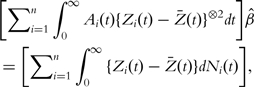(4)

where . Denote

Denote the ( j,l )^th element of Lⁱ as , and the j^th component of Rⁱ and β as and β_j, respectively. Equation (4) is equivalent to the following d equations:

(5)

Motivated by (5), Ma and Huang [16] proposed the following objective function

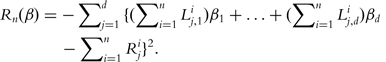(6)

Examples of using the additive risk model in prognosis studies with microarrays include [16–19] and others.

AFT model

Both the Cox and additive risk models describe the survival hazard. In contrast, the AFT model describes the event time directly [13, 14]. The AFT model assumes

(7)

where α is the intercept and ε is the random error with an unknown distribution. Here, the log transformation can be replaced with other monotone transformations.

Estimation of the AFT model has been extensively studied. Several available approaches, including the Buckley-James approach [20] and rank-based approaches [21], suffer from a high computational cost when there are a large number of covariates. A computationally more affordable approach is the weighted least squares approach [22].

With slight abuse of notation, define . Denote 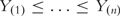as the ordered Y_is. Denote δ_(i) and Z_(i) as the censoring indicator and covariate associated with Y_(i). Let be the Kaplan-Meier estimate of the distribution function F of log(T), which can be computed as . Here w_is are computed as

With the weighted least squares approach, the objective function is

(8)

Examples of using the AFT model in prognosis studies with microarrays include [9, 23–26] and others.

Remarks

Denote S(t) as the survival function at time t. Denote S¹(t) and S²(t) as the survival functions for covariate values Z and Z + 1. Under the Cox model, log(−log(S¹(t))−log(−log(S²(t)) is a constant; under the additive risk model, log(S¹(t))−log(S²(t))/t is a constant; Under the AFT model, a linear relationship between log(t) and covariates can be observed. Such observations have been used to develop graphic diagnosis tools when there are a small number of covariates [4, 8].

For all the three models, when d <<n, is a consistent estimate of β. An attractive feature of R_n(β) is that it only involves β but not the nonparametric parameter. That is, although the three models are much more flexible than parametric models, they have similar computational cost as parametric models. We refer to [27, 28] for thorough discussions of the three models.

There are other semiparametric prognosis models, including the proportional odds model, general transformation model, accelerated hazards model and others. Those models are not widely used, and hence will not be considered.

GENE SELECTION AND MODEL EVALUATION

Gene selection using Lasso

Among the thousands of genes surveyed in microarray studies, only a subset are associated with disease prognosis. Hence, variable selection is needed along with model estimation.

Among the many available variable selection techniques, penalization methods have attracted special attention. The most famous penalization methods are perhaps the AIC and BIC, which penalize the number of unknown parameters in likelihood approaches and have been extensively used in biomedical studies. Examples of penalization methods in microarray prognosis studies include [9–11, 16, 23, 24, 29–31] and many others.

When there are a large number of covariates, the AIC and BIC may be unstable and suffer from high computational cost. An alternative penalization approach that has better statistical properties is the Lasso [32], where the estimate is defined as

(9)

Here R_n is defined in (2), (6) and (8), β_j is the j^th component of β, and M is the data-dependent tuning parameter.

The Lasso controls complexity of the model by controlling the norms of regression coefficients. It is a special case of the bridge-type penalty defined as When γ = 0, this penalty becomes the AIC/BIC-type penalty; When γ = 2, this penalty becomes the ridge penalty, which has a long history for ill-designed models but cannot conduct variable selection. We refer to Ma and Huang [6], Tibshrani [32], and Zhang and Huang [33] for more detailed discussions of the Lasso and other penalization methods. We note that, the Lasso approach is ‘independent’ of the model and objective function. It can be directly applied to the three prognosis models. We adopt the Lasso for gene selection, because it is the most extensively used approach, has affordable computational cost, and has served as benchmark in many studies. In addition, Zhang and Huang [33] and several other studies have established that, with a high probability, the Lasso is capable of selecting all genes associated with disease outcomes. This is further confirmed by our simulation study presented below. Thus, the Lasso seems to be a proper choice for gene selection. The Lasso has been used in cancer prognosis studies with microarrays under the Cox [10], additive risk [16], and AFT [23] models. The R package ‘penalized’ has been developed to compute the Lasso estimates (we refer to http://cran.r-project.org/web/packages/penalized/penalized.pdf for more information).

In this study, we use the boosting approach to compute the Lasso estimate [34]. The Lasso involves a tuning parameter M, which balances goodness-of-fit and sparsity and will be selected using V-fold cross validation.

Evaluation

In simulation, the true generating model is known and independent testing data can be generated. Thus, it is easy to evaluate gene identification and prediction performance.

Analysis of real data can provide more relevant information than simulation [35]. In analysis of real data, with limited understanding of genomic mechanisms underlying disease prognosis, we are unable to determine which model selects biologically the most meaningful genes. Instead, we consider the following statistical evaluation/comparison techniques.

Evaluation of prediction performance

An important goal of genomic studies is to make prediction using identified gene signatures. In addition, prediction performance can provide an indirect assessment of gene identification results—if genes identified are biologically more meaningful, prediction using those genes should be more accurate. Ideally, prediction evaluation should use independent datasets. However, for most genomic studies, it is hard to find independent studies with comparable designs.

We use the Leave-One-Out (LOO) cross validation-based approach for prediction evaluation. For i = 1 … n, (i) remove subject i from data; (ii) compute the estimate using the rest n−1 subjects. To ensure a fair evaluation, supervised gene screening (if any) and tuning parameter selection need to be conducted with the reduced data. (iii) Compute the predictive risk score ; and (iv) repeat steps (i)–(iii) over all n subjects. Dichotomize the n predictive risk scores at the median and create two risk groups. Compute the logrank statistic, which measures difference of survival between the two groups. Under the null, the logrank statistic is χ² distributed with degree of freedom 1. A significant logrank statistic indicates that the genes selected under a specific model have satisfactory predictive power [4, 28]. The logrank statistic and its significance level can be computed using several available software, for example Proc Lifetest in SAS or the ‘survival’ package in R.

Evaluation of reproducibility

The approach described above assesses performance of all identified genes combined. Reproducibility of each identified gene is also of significant interest. Ideally, reproducibility evaluation should be based on analysis of multiple independent datasets. Without such data, we again resort to cross validation.

We consider the following approach: (i) remove one subject from data; (ii) conduct regularized estimation and gene selection using the reduced data with sample size n−1; (iii) repeat steps (i) and (ii) over all subjects. For each gene, count c, the number of times it is identified in the n models. The ratio c/n provides a measure of reproducibility, and is referred to as the ‘occurrence index’ in the literature [16]. The reproducibility evaluation is a byproduct of the prediction evaluation, and does not incur any additional computational cost.

Under a specific model, the Lasso can identify a set of genes using all observations. We are interested in evaluating whether those genes have reasonably high occurrence indexes, and whether their occurrence indexes are higher than those not identified. This evaluation can reveal whether a specific prognosis model (with the Lasso) can identify the most reproducible genes.

NUMERICAL STUDIES

Simulation

We conduct simulation and investigate performance of different models under different data generating models. We generate 500 genes, whose marginal distributions are normal. Expressions of genes i and j have correlation coefficient ρ^|i–j|, with ρ = 0.1 (weak correlation) or 0.6 (strong correlation). We generate a training set and a testing set, each with sample size 100. The event times are generated from the Cox, additive risk and AFT models. The censoring times are generated from exponential distributions. We adjust the censoring distribution so that the censoring rate is about 50%. Among the 500 genes, the first 15 have nonzero regression coefficients, i.e. are associated with disease prognosis. For each training set, we apply the three models and use Lasso for gene selection. We then make prediction for subjects in the testing set. Specifically, for each subject in the testing set, we compute the predictive risk score. We then create two risk groups by dichotomizing the risk scores, and compute the logrank statistic.

We compute summary statistics based on 500 replicates and present the results in Table 1. We can see that when the assumed model matches the true underlying model, a majority or all of the true positives can be identified. For example, when genes have weakly correlated expressions and both the assumed and true models are Cox models (row 1 of Table 1), the Lasso identifies all the 15 true positives. The logrank statistic is highly significant, indicating satisfactory prediction performance. In contrast, under model misspecification, the Lasso fails to identify the true positives. For example, when the true model is the Cox model but the additive risk model is assumed (row 2), only 4 true positives are identified.

Table 1:

Simulation study: median computed based on 500 replicates

True model	Correlation	Assumed model	Positive	True positive	P-value
Cox	0.1	Cox	27	15	< 0.0001
		Additive	36	4	0.153
		AFT	50	5	0.306
	0.6	Cox	18	15	< 0.0001
		Additive	38	8	< 0.001
		AFT	40	4	0.020
Additive	0.1	Cox	40	5	0.418
		Additive	25	13	0.023
		AFT	10	0	0.731
	0.6	Cox	40	5	0.231
		Additive	22	13	0.012
		AFT	10	0	0.402
AFT	0.1	Cox	27	10	< 0.0001
		Additive	25	8	0.006
		AFT	26	14	< 0.0001
	0.6	Cox	17	9	< 0.001
		Additive	13	5	0.002
		AFT	22	15	< 0.0001

Positive: number of genes identified; true positive: number of identified genes truly associated with disease; P-value: P-value of the logrank statistic.

Cancer microarray studies

DLBCL study

Rosenwald et al. [36] reported a diffuse large B-cell lymphoma (DLBCL) prognosis study. This study retrospectively collected tumor biopsy specimens and clinical data for 240 patients with untreated DLBCL. The median follow up is 2.8 years, with 138 observed deaths. Lymphochip cDNA microarray is used to measure the expressions of 7399 genes. Raw data and detailed experiment protocol are available at http://llmpp.nih.gov/DLBCL/.

MCL study

Rosenwald et al. [37] reported a study using microarray gene expression analysis in mantle cell lymphoma (MCL). Among 101 untreated patients with no history of previous lymphoma, 92 were classified as having MCL based on established morphologic and immunophenotypic criteria. Survival times of 64 patients were available and 28 patients were censored. The median survival time was 2.8 years (range 0.02–14.05 years). Lymphochip DNA microarrays were used to quantify mRNA expressions in the lymphoma samples from the 92 patients. Gene expression data that contains expression values of 8810 cDNA elements is available at http://llmpp.nih.gov/MCL.

Breast cancer study

Breast cancer is the second leading cause of death from cancer among women in the United States. Despite major progress in breast cancer treatment, the ability to predict metastasis of the tumor remains limited. van’t Veer et al. [38] reported a breast cancer prognosis study investigating the time to distant metastasis. 97 lymph node-negative breast cancer patients, 55 years old or younger, participated in this study. Among them, 46 developed distant metastases within 5 years. Expression levels for 24 481 gene probes were collected. Data is available at http://www.rii.com/publications/2002/vantveer.html.

Data processing

For all the three datasets, we fill in missing expressions using medians across all samples. We normalize gene expressions to have median zero and variance one. In addition, to reduce computational cost, we conduct the following supervised screening. Using uncensored observations, we compute the correlation coefficient between event time and each gene expression. We select 500 genes with the largest absolute values of correlation coefficients. Since the number of genes associated with prognosis is expected to be much smaller than 500, the supervised screening should lead to very few false negatives. Of note, to ensure a fair evaluation, the supervised screening needs to be conducted for each reduced dataset with one observation removed.

Data analysis results

We analyze the three datasets under the three prognosis models. We use the Lasso for regularized estimation and gene selection. The tuning parameter M is selected using 5-fold cross validation.

Gene identification

We show the summary of gene identification results under different prognosis models in Table 2. We can see that, under each model, a small number of genes are identified. The most interesting observation is that gene sets identified under different models have little or even no overlap. For example, for the DLBCL data, under the Cox and additive risk models, 39 and 25 genes are identified, respectively. However, there are only 5 genes in common. We conclude from Table 2 that ‘gene identification results are model-dependent’.

Table 2:

Number of genes identified and overlap under different models

		Cox	Additive	AFT
DLBCL	Cox	39	5	7
		Additive		25	2
		AFT			49
MCL	Cox	37	4	9
	Additive		20	1
		AFT			55
Breast	Cox	21	2	2
		Additive		13	0
		AFT			25

It has been hypothesized that although genes identified using different approaches (or under different models) are different, they may belong to the same pathways and/or represent the same biological processes. Our knowledge of genes’ biological functions is still very limited. For example, when searching the KEGG, we are only able to find pathway information for less than half of the genes for the three datasets. In addition, genes, as opposed to pathways or biological processes, are still the most commonly used functional units in genomic studies. Thus, we focus on comparing identification results at the gene level.

Evaluation of prediction

We use the LOO approach to evaluate prediction performance of genes identified under different models. The logrank statistics are shown in Table 3. We can see that for the DLBCL and MCL data, prediction under all the three models is satisfactory (P-value < 0.05). For the Breast cancer data, prediction under the Cox and additive models is satisfactory (P-value < 0.05). The most interesting observation is that, if we use the logrank statistic—which measures prediction performance—as the criterion for model selection, ‘the three datasets have three different optimal models’.

Table 3:

Evaluation of prediction: Logrank statistics under different models

	Cox	Additive	AFT
DLBCL	10.0	6.03	12.50
MCL	18.10	13.10	4.80
Breast	4.23	10.00	3.78

A logrank statistic greater than 3.84 is significant at the 0.05 level.

Evaluation of reproducibility

We use the LOO approach to evaluate reproducibility, and show the summary statistics of occurrence indexes in Table 4. We can see that the genes identified using all observations have reasonably high occurrence indexes. In contrast, genes not identified have much lower occurrence indexes. We also see that all models miss a few genes with high occurrence indexes. In addition, ‘if occurrence index, which is a measure of reproducibility, is chosen as the criterion for model selection, the Cox model outperforms the other two’.

Table 4:

Occurrence Index under different models: median [range]

		Cox	Additive	AFT
DLBCL	Selected	0.996 [0.213, 1]	0.458 [0.008, 0.979]	0.971 [0.2, 1]
	Not selected	0 [0, 0.696]	0 [0, 0.554]	0 [0, 0.592]
MCL	Selected	0.978 [0.152, 1]	0.902 [0.239, 0.978]	0.848 [0.207, 1]
	Not selected	0 [0, 0.609]	0 [0, 0.467]	0 [0, 0.652]
Breast	Selected	0.990 [0.835, 1]	0.484 [0.021, 0.928]	0.845 [0.598, 1]
	Not selected	0 [0, 0.814]	0 [0, 0.608]	0 [0, 0.474]

Selected: genes selected using all observations.

In some studies, it has been suggested that the most reproducible genes should be selected as markers. Since the occurrence index provides a way of evaluating reproducibility, we also look into gene selection using reproducibility as the criterion. For each dataset, we select the 20 most reproducible genes under each model and evaluate overlap. We find that the sets of most reproducible genes are also model-dependent. For example for the DLBCL data, the numbers of overlapping genes are 3 (Cox and Additive), 3 (Cox and AFT) and 1 (Additive and AFT), respectively. Analyses of the MCL and Breast cancer data lead to similar results. We conclude that ‘selecting genes based on reproducibility cannot change the model-dependent nature of gene selection’.

DISCUSSION

A major goal of genomic studies is to identify disease markers. Although great effort has been devoted to development of gene selection techniques, insufficient attention has been paid to the assumed prognosis models. In this article, we review the three most extensively used semiparametric prognosis models. We conduct simulation and find that model misspecification can lead to unsatisfactory gene identification results. We analyze three datasets under the three models, and find that gene identification results, prediction performance and reproducibility are model-dependent. Thus, we suggest that in practical data analysis, researchers should examine multiple prognosis models.

To the best of our knowledge, there is still no consensus on how to select the optimal model under the ‘large d, small n’ setup. The biological implications of identified genes may be the ultimate selection criterion. However, genomic research is still at the discovery stage. Our limited knowledge has forced us to consider statistical, as opposed to biological, comparison and evaluation. In this article, we use the LOO approaches for evaluation of prediction and reproducibility. The logrank statistic and the occurrence index are proposed as the evaluation/comparison criteria.

Among the three prognosis models, the Cox and AFT models belong to the family of transformation models. Theoretically speaking, it is possible to fit a general transformation model and then determine whether the Cox or the AFT model is more proper. In an unpublished study, we experimented with this approach and found that the estimation results were unsatisfactory even with a moderate number of covariates. In addition, such an approach cannot determine whether the additive risk model holds.

Our presentation is in the context of microarray studies and we focus on analysis of cancer data. We expect similar conclusions to hold for other profiling platforms and other diseases. We adopt the Lasso for gene selection. We expect that adopting other penalties or other selection methods may change some minor details but not the model-dependent nature of gene selection and prediction performance.

Our literature review suggests that prognosis models other than the Cox model and penalized gene selection have been extensively used in statistical and bioinformatics studies. However, we are unable to find such applications in medical studies. The unfortunate lag between the development of new statistical technologies and their medical applications has been well noted [39]. Given their satisfactory performance demonstrated in statistical studies, we expect the additive risk model, AFT model, and Lasso approach to be used in medical studies in the near future.

Key Points.

• Multiple prognosis models have been used in genomic studies.

• Our numerical studies show that the gene identification results, predictive performance and reproducibility of identified genes are model-dependent.

• Researchers should explore multiple prognosis models in practical data analysis.

• There is a critical need for model diagnosis and selection methods for high-dimensional genomic data.

FUNDING

National Institutes of Health [LM009754 and CA120988 to S.M. and J.H.].

Biographies

Shuangge Ma obtained his PhD in Statistics from University of Wisconsin in 2004. He is an Assistant Professor in the School of Public Health, Yale University.

Jian Huang obtained his PhD in Statistics from University of Washington in 1994. He is a Professor in the Department of Statistics and Actuarial Sciences and the Department of Biostatistics, University of Iowa.

Mingyu Shi obtained her PhD in Engineering from University of California, Berkeley, in 2008. She is a Quantitative Analyst at Standard and Poor’s.

Yang Li is a PhD candidate in the School of Statistics, Renmin University, China. He is currently under a joint training program in the School of Public Health, Yale University.

Ben-Chang Shia is a Professor of Statistics and Information Science in Fu Jen Catholic University and the Director-General of the Chungha Data Mining Society.

References

- Knudsen S. Cancer Diagnostics with DNA Microarrays. Hoboken, New Jersey: John Wiley & Sons; 2006. [Google Scholar]
- Sun G. Application of DNA microarrays in the study of human obesity and type 2 diabetes. OMICS. 2007;11:25–40. doi: 10.1089/omi.2006.0003. [DOI] [PubMed] [Google Scholar]
- Cox DR. Regression models and life-tables. J R Stat Soc Series B Stat Methodol. 1972;34:187–220. [Google Scholar]
- Klein JP, Moeschberger ML. Survival Analysis. Springer; 2003. [Google Scholar]
- Dai J, Lieu L, Rocke D. Dimension reduction for classification with gene expression microarray data. Stat Appl Genet Mol Biol. 2009;5:6. doi: 10.2202/1544-6115.1147. [DOI] [PubMed] [Google Scholar]
- Ma S, Huang J. Penalized feature selection and classification in bioinformatics. Brief Bioinform. 2008;9:392–403. doi: 10.1093/bib/bbn027. [DOI] [PMC free article] [PubMed] [Google Scholar]
- van Wieringen WN, Kun D, Hampel R, et al. Survival prediction using gene expression data: a review and comparison. Comput Stat Data Anal. 2009;53:1590–603. [Google Scholar]
- Fleming TR, Harrington DP. Counting Processes and Survival Analysis. Wiley Interscience; 1991. [Google Scholar]
- Engler D, Li Y. Survival analysis with high-dimensional covariates: an application in microarray studies. Stat Appl Genet Mol Biol. 2009;8:14. doi: 10.2202/1544-6115.1423. [DOI] [PMC free article] [PubMed] [Google Scholar]
- Gui J, Li H. Penalized Cox regression analysis in the high-dimensional and low-sample size settings, with applications to microarray gene expression data. Bioinformatics. 2005;21:3001–8. doi: 10.1093/bioinformatics/bti422. [DOI] [PubMed] [Google Scholar]
- Ma S, Huang J, Shen S. Identification of cancer-associated gene clusters and genes within clusters via clustering penalization. Stat Interface. 2009;2:1–11. doi: 10.4310/sii.2009.v2.n1.a1. [DOI] [PMC free article] [PubMed] [Google Scholar]
- Shoemaker JS, Lin SM. Methods of Microarray Data Analysis IV. Springer; 2004. [Google Scholar]
- Breslow NE, Day NE. Statistical Models in Cancer Research, 2. Lyon: IARC; 1987. [Google Scholar]
- Therneau TM, Grambsch RM. Modeling Survival Data: Extending the Cox Model. Springer; 2001. [Google Scholar]
- Lin DY, Ying Z. Semiparametric analysis of the additive risk model. Biometrika. 1994;81:61–71. [Google Scholar]
- Ma S, Huang J. Additive risk survival model with microarray data. BMC Bioinformatics. 2007;8:192. doi: 10.1186/1471-2105-8-192. [DOI] [PMC free article] [PubMed] [Google Scholar]
- Ma S, Kosorok MR, Fine JP. Additive risk models for survival data with high-dimensional covariates. Biometrics. 2006;62:202–10. doi: 10.1111/j.1541-0420.2005.00405.x. [DOI] [PubMed] [Google Scholar]
- Martinussen T, Scheike TH. The additive hazards model with high-dimensional regressors. Lifetime Data Anal. 2009;15:330–42. doi: 10.1007/s10985-009-9111-y. [DOI] [PubMed] [Google Scholar]
- Zhao Y, Zhou Y, Zhao M. Analysis of additive risk model with high-dimensional covariates using partial least squares. Stat Med. 2009;28:181–93. doi: 10.1002/sim.3412. [DOI] [PubMed] [Google Scholar]
- Buckley J, James I. Linear regression with censored data. Biometrika. 1979;66:429–36. [Google Scholar]
- Ying ZL. A large sample study of rank estimation for censored regression data. Ann Stat. 1993;21:76–99. [Google Scholar]
- Stute W. Nonlinear censored regression. Stat Sin. 1999;9:1089–102. [Google Scholar]
- Datta S, Le-Rademacher J, Datta S. Predicting patient survival from microarray data by accelerated failure time modeling using partial least squares and LASSO. Biometrics. 2007;63:259–71. doi: 10.1111/j.1541-0420.2006.00660.x. [DOI] [PubMed] [Google Scholar]
- Huang J, Ma S, Xie H. Regularized estimation in the accelerated failure time model with high dimensional covariates. Biometrics. 2006;62:813–20. doi: 10.1111/j.1541-0420.2006.00562.x. [DOI] [PubMed] [Google Scholar]
- Schmid M, Hothorn T. Flexible boosting of accelerated failure time models. BMC Bioinformatics. 2008;9:269. doi: 10.1186/1471-2105-9-269. [DOI] [PMC free article] [PubMed] [Google Scholar]
- Sha N, Tadesse MG, Vannucci M. Bayesian variable selection for the analysis of microarray data with censored outcomes. Bioinformatics. 2006;22:2262–8. doi: 10.1093/bioinformatics/btl362. [DOI] [PubMed] [Google Scholar]
- D’Agostino RB. Tutorials in Biostatistics. Vol. 1. John Wiley & Sons; 2005. [Google Scholar]
- Lee ET, Go OT. Survival analysis in public health research. Annu Rev Public Health. 1997;18:105–34. doi: 10.1146/annurev.publhealth.18.1.105. [DOI] [PubMed] [Google Scholar]
- Binder H, Schumacher M. Allowing for mandatory covariates in boosting estimation of sparse high-dimensional survival models. BMC Bioinformatics. 2008;9:14. doi: 10.1186/1471-2105-9-14. [DOI] [PMC free article] [PubMed] [Google Scholar]
- Segal MR. Microarray gene expression data with linked survival phenotypes: diffuse large-B-cell lymphoma revisited. Biostatistics. 2006;7:268–85. doi: 10.1093/biostatistics/kxj006. [DOI] [PubMed] [Google Scholar]
- Zhu J, Hastie T. Classification of gene microarrays by penalized logistic regression. Biostatistics. 2004;5:427–44. doi: 10.1093/biostatistics/5.3.427. [DOI] [PubMed] [Google Scholar]
- Tibshrani R. Regression shrinkage and selection via the lasso. J R Stat Soc Series B Stat Methodol. 1996;58:267–88. [Google Scholar]
- Zhang CH, Huang J. The sparsity and bias of the Lasso selection in high-dimensional linear regression. Ann Stat. 2008;4:1567–94. [Google Scholar]
- Kim Y, Kim J. In: Proceedings of the 21st International Conference on Machine Learning. Banff, Alberta, Canada: ICML; 2004. Gradient LASSO for feature selection. [Google Scholar]
- Rocke DM, Ideker T, Troyanskaya O, et al. Papers on normalization, variable selection, classification or clustering of microarray data. Bioinformatics. 2009;25:701–2. [Google Scholar]
- Rosenwald A, Wright G, Chan W, et al. The use of molecular profiling to predict survival after chemotherapy for diffuse large-B-cell lymphoma. N Engl J Med. 2002;346:1937–47. doi: 10.1056/NEJMoa012914. [DOI] [PubMed] [Google Scholar]
- Rosenwald A, Wright G, Wiestner A, et al. The proliferation gene expression signature is a quantitative integrator of oncogenic events that predicts survival in mantle cell lymphoma. Cancer Cell. 2003;3:185–97. doi: 10.1016/s1535-6108(03)00028-x. [DOI] [PubMed] [Google Scholar]
- van’t Veer LJ, Dai H, van de Vijver MJ, et al. Gene expression profiling predicts clinical outcome of breast cancer. Nature. 2002;415:530–6. doi: 10.1038/415530a. [DOI] [PubMed] [Google Scholar]
- Obrams GI, Hjortland M. The application of developments in theoretical biostatistics to epidemiologic research. Stat Med. 1992;12:789–93. doi: 10.1002/sim.4780120807. [DOI] [PubMed] [Google Scholar]