Sidelobe Suppression in Ultrasound Imaging using Dual Apodization with Cross-correlation

Abstract

This paper introduces a novel sidelobe and clutter suppression method in ultrasound imaging called Dual Apodization with Cross-correlation or DAX. DAX dramatically improves the contrast-to-noise ratio (CNR) allowing for easier visualization of anechoic cysts and blood vessels. This technique uses dual apodization or weighting strategies that are effective in removing or minimizing clutter and efficient in terms of computational load and hardware/software needs. This dual apodization allows us to determine the amount of mainlobe versus clutter contribution in a signal by cross-correlating RF data acquired from two apodization functions. Simulation results using a 128 element 5 MHz linear array show an improvement in CNR of 139 % compared to standard beamformed data with uniform apodization in a 3 mm diameter anechoic cylindrical cyst. Experimental CNR using a tissue-mimicking phantom with the same sized cyst shows an improvement of 123 % in a DAX processed image.

I. INTRODUCTION

The goal of beamforming is to focus ultrasound energy to one location only, but this is not truly achievable with standard delay and sum beamforming. This gives rise to off-axis sidelobes and clutter. These sidelobes or clutter inherent in ultrasound imaging are undesirable side effects since they degrade image quality by lowering CNR and the detectability of small targets. Improving the contrast of ultrasound has many clinically significant applications. In breast ultrasound, the main purpose is to differentiate solid and cystic masses [1]. Simple anechoic cysts with fill-in caused by multiple scattering, reverberations and clutter can be misclassified as malignant lesions. Levels of fill-in are increased in the presence of aberrations caused by intermittent layers of fat and tissue. Delineation of carcinoma may also be improved with better signal processing methods that improve contrast. Similar problems arise when imaging other soft tissue. For hepatic imaging, visualization of cystic liver lesions and dilated bile ducts can be improved [2]. The visualization of prostate cancer may be improved since prostate cancer is usually hypoechoic [3]. One way to improve CNR is to reduce sidelobe and clutter levels by applying a weighting or shaping function such as a Hanning or Hamming apodization across the transmit and receive apertures. These types of weighting functions are called linear apodization functions since the same weighting is applied to the aperture independent of depth or of imaging line. As a trade-off, they lower the sidelobes at the expense of worse mainlobe lateral resolution. To avoid making this trade-off, there have been several publications in nonlinear sidelobe suppression methods which aim for little or no loss in mainlobe resolution while achieving low clutter levels commonly associated with apodization [4] – [7].

In recent work, Guenther and Walker developed optimal apodization functions using constrained least squares theory [4], [5]. This method creates apodization functions with the goal of limiting the energy of the point spread function (PSF) outside a certain area and maintaining a peak at the focus. A point target simulation was performed using a linear array with 192 elements with 200 µm element pitch and a transmit frequency of 6.5 MHz. Using this method, a 5–10 dB reduction in sidelobe levels compared to a Hamming apodization was achieved. Wang used a comparator to select the minimum magnitude from two or more sets of data using various apodization methods, such as uniform, Hanning or Hamming [6]. By taking the minimum magnitude on a pixel-by-pixel basis, this method preserves the mainlobe resolution of the uniformly apodized data and lowers sidelobes similar to a Hanning or Hamming apodized data. Stankwitz developed a spatially variant nonlinear apodization (SVA) technique, which uses the lateral phase differences between Hanning and uniformly apodized data to distinguish between mainlobe and clutter signals. This is accomplished by taking advantage of the properties of raised-cosine weighting functions and finding the optimal apodization function on a pixel-by-pixel basis [7].

An ideal contrast improvement method would greatly improve contrast such that lesions are easily visualized without significantly increasing computational complexity, worsening lateral and/or temporal resolution. In this paper, we present a target-dependent clutter suppression method using pairs of apodization functions. By using certain pairs of apodization functions, we can pass mainlobe signals and attenuate clutter signals using normalized cross-correlation coefficients of RF signals in the axial direction. The amount of attenuation is proportional to the amount of clutter in the signal. A target-dependent weighting matrix is created that will be multiplied to the standard beamformed image. In a point target simulation, using a linear array with 128 elements with element pitch of 308 µm and a transmit frequency of 5 MHz, this technique lowers clutter levels by over 40 dB compared to standard beamformed data with a uniform apodization while keeping the same mainlobe resolution with a minimal computation load.

II. DESIGNS

Assuming linearity, any ultrasound echo signal can be thought of as the sum of two signals: one signal is the mainlobe contribution which is desired and one signal from the sidelobes, grating lobes, and other forms of clutter which reduces image contrast. The amount of mainlobe contribution and sidelobe contribution depends on two factors: 1) the ratio of the mainlobe amplitude to the sidelobe amplitude and 2) the strength of the scatterers within the mainlobe versus the strength of the scatterers in the clutter region. To improve contrast, one would like to remove or at least minimize contributions from clutter. Our approach to removing clutter is to distinguish the mainlobe dominated signals from clutter signals by developing two point spread functions using two different apodization functions. These two apodization functions give similar mainlobe signals and very different clutter patterns. Therefore, echoes from a target, such as speckle or a point target, which comprises primarily of mainlobe components will look similar to each other, but echoes from a target, such as a cyst, which are mainly clutter will appear different from each other. Signals from a target which consists of a comparable contribution from both mainlobe and clutter will be partially similar.

The degree of similarity can be quantified using normalized cross-correlation between the two signals RX1 and RX2 from two PSFs. Normalized cross-correlation (NCC) is performed using segments of RF data along the axial direction at zero lag. The normalized cross-correlation coefficient ρ at zero lag is calculated for every sample and used as a target-dependent pixel-by-pixel weighting matrix, which passes mainlobe dominated signals and attenuates clutter dominated signals (1). The post beamformed RF data is then multiplied by this weighting matrix.

$$\rho (i,j)=\frac{{\displaystyle \sum _{k=i-A}^{i+A}\mathit{\text{RX}}1(k,j)\mathit{\text{RX}}2(k,j)}}{\sqrt{{\displaystyle \sum _{k=i-A}^{i+A}\mathit{\text{RX}}1{(k,j)}^2}}\sqrt{{\displaystyle \sum _{k=i-A}^{i+A}\mathit{\text{RX}}2{(k,j)}^2}}}$$ (1)

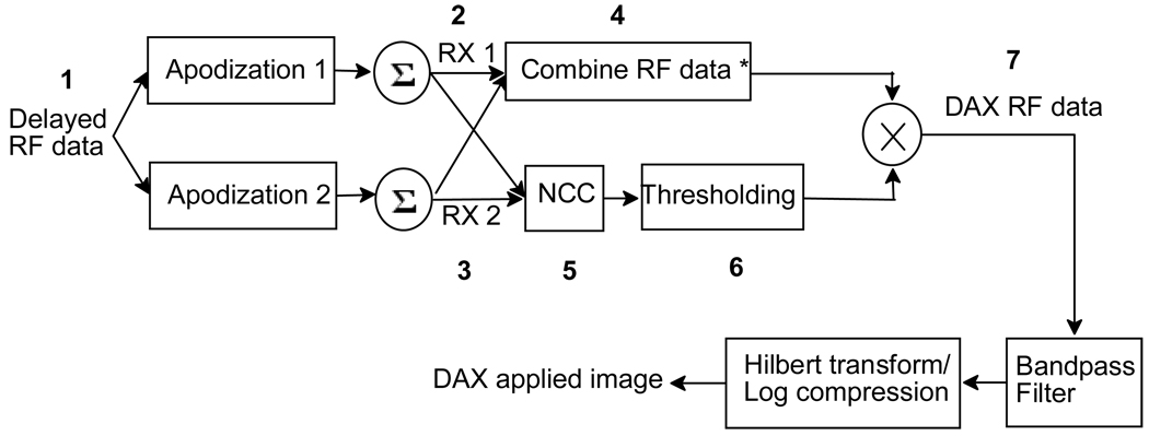
In (1), index i indicates the i^th sample in image line j. The total cross-correlation segment length is 2A+1 samples. Normalized cross-correlation coefficients range from −1 to 1. Two signals are identical if the cross-correlation coefficient is 1 and they are considered uncorrelated if the coefficient is near or below zero. Signals would be somewhat correlated if ρ is in between 0 and 1. In the proposed method, if the coefficient is greater than or equal to a set threshold value ε > 0, then the sample value will be multiplied by the cross-correlation coefficient. If the coefficient is less than the threshold value ε, the sample value is multiplied by the threshold value ε. This algorithm is called dual apodization with cross-correlation or DAX. A general system block diagram is shown in Fig. 1.

Fig. 1.

General system block diagram for dual apodization with cross-correlation (DAX). Numbers indicate steps described in the text. RX1 and RX2 are two data sets created with two apodization functions. * The combined RF data can be obtained by taking the minimum magnitude of RX1 and RX2 or the sum of RX1 and RX2.

In Fig. 1, the delayed data is processed with two receive apodization functions to create beamformed RF data sets RX1 and RX2. RX1 and RX2 can be combined in different ways. One way to combine is through a minimum function as done in dual apodization described by Wang and Fienup [6, 7]. This min function is used to select the minimum magnitude at each sample between the two data sets. Another way to combine is to add them. This is the case when the two apodization functions are complementary shown later in this section. Simply adding the two data sets from the complementary apodization functions would give us the same data from a standard receive aperture. If the cross-correlation value is less than a threshold value ε, the value will be replaced with the set threshold value (2). This signal is considered to be mainly clutter and needs to be suppressed. Signals having a comparable mixture of mainlobe and clutter will receive a reduction in amplitude between ε and 1. The cross-correlation matrix is multiplied to the combined RF data (* in Fig. 1)

$$\text{DAX CC}=\{\begin{array}{cc}\rho ,\hfill & \rho >=\epsilon \hfill \\ \epsilon ,\hfill & \rho <\epsilon \hfill \end{array}$$ (2)

where ρ is calculated using (1).

The detailed steps to acquire a DAX processed image are as follows:

1. A subaperture (in this paper, 64 elements) transmits a focused beam into the target. Echoes are collected from the same 64 elements.

2. In receive, we beamform using our first apodization function to create dataset RX1.

3. Likewise, a second apodization function is used to create dataset RX2.

4. These two data sets are used to create the combined RF data (* in Fig. 4). The combined RF data can be obtained by taking the minimum magnitude of RX1 and RX2 or the sum of RX1 and RX2.

5. A cross-correlator calculates a normalized cross-correlation value for each pixel. Typically 2–3 wavelengths are used as a segment size for cross-correlation.

6. The value is sent to a thresholding operator. If the value is less than or equal to ε, then replace it with ε. If it is greater than ε, then leave it unchanged.

7. The resulting cross-correlation matrix is multiplied by the combined RF data from step 4.

8. The DAX RF data can undergo further signal processing such as bandpass filtering, envelope detection, log-compression, and scan conversion.

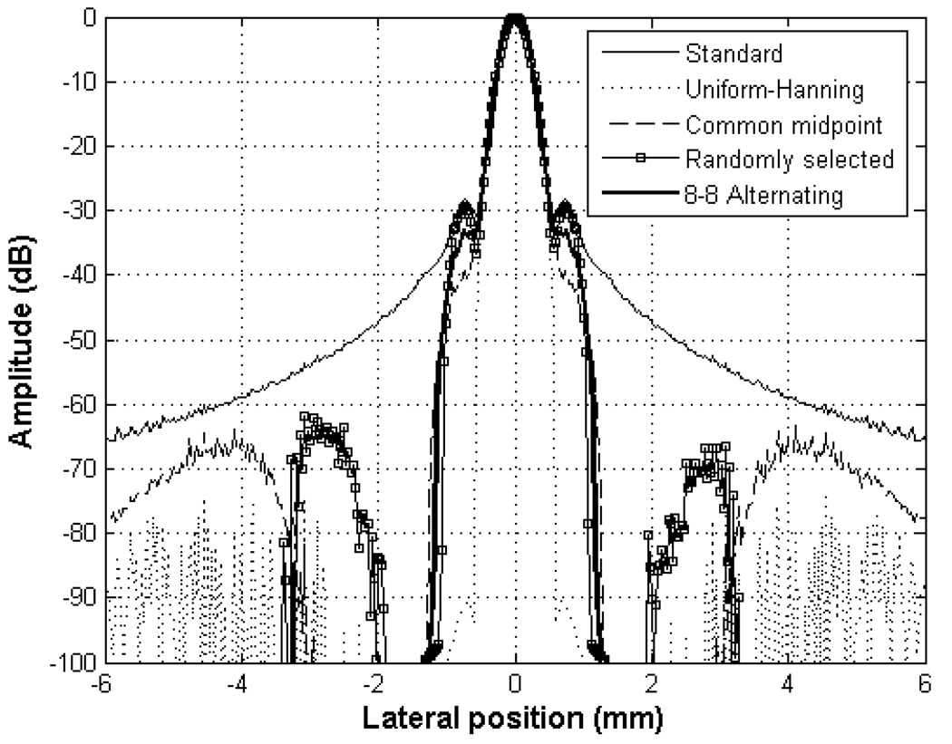
Fig. 4.

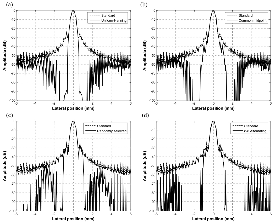
Lateral Beamplots comparing four DAX schemes with standard beamformed data with uniform apodization.

We investigated the performance of four pairs of apodization functions, where each pair has a well correlated mainlobe response and a different or uncorrelated sidelobe response. All methods use echo datasets formed from each apodization and calculate a weighting matrix by cross-correlating image pairs. All apodization pairs have the same goal of suppressing clutter levels, thus increasing CNR, while maintaining mainlobe resolution.

A. Apodization Scheme 1: Uniform and Hanning

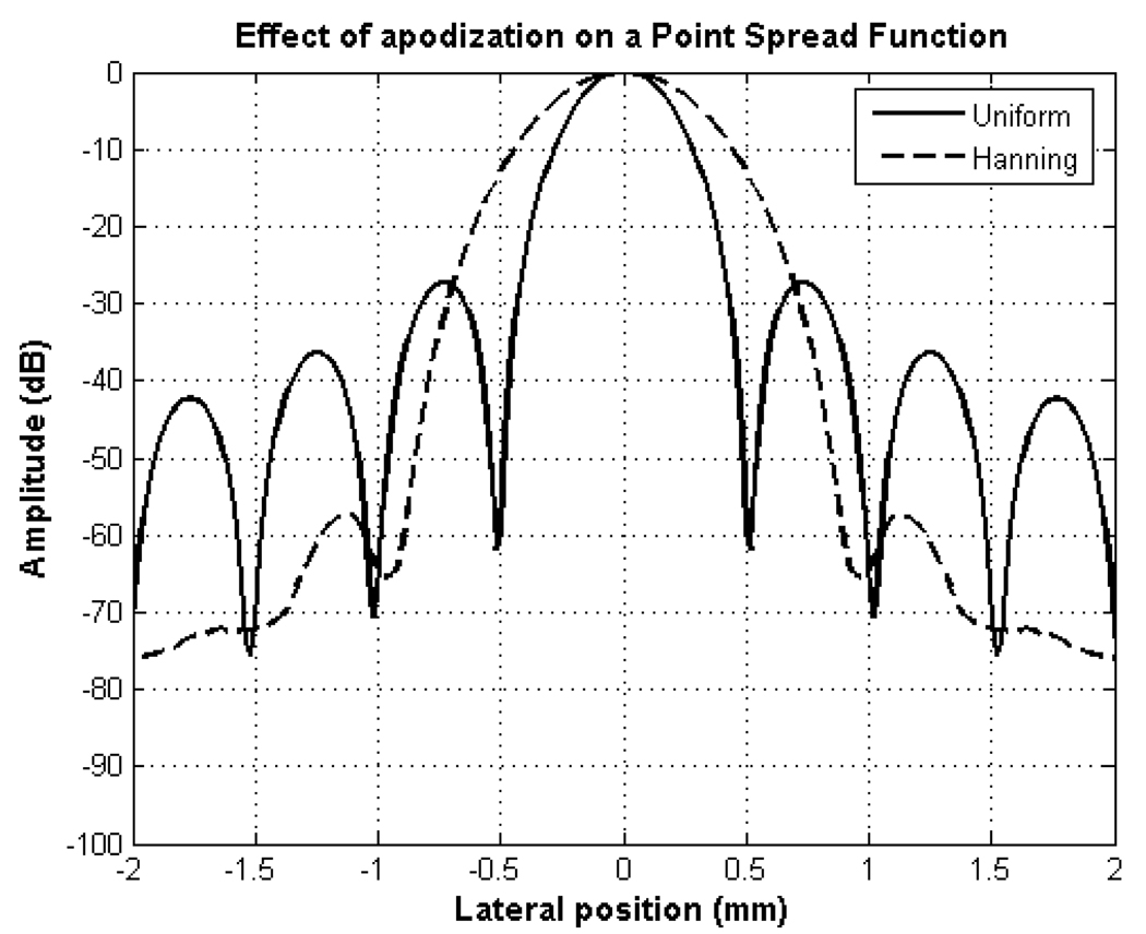
Motivated by Stankwitz [7], our first choice is using a pair of apodization functions that are common in ultrasound imaging practice. An aperture with a uniform amplitude weighting or a rect apodization function gives a sinc function shaped beam. This will lead to sidelobes at −26 dB. With an apodization function smoother than uniform apodization such as Hanning apodization, the sidelobe level is lowered from −26 dB to −57 dB but has a larger −6 dB beamwidth compared to uniform weighting (Fig. 2).

Fig. 2.

Uniform and Hanning weighted apertures in continuous wave (CW) mode.

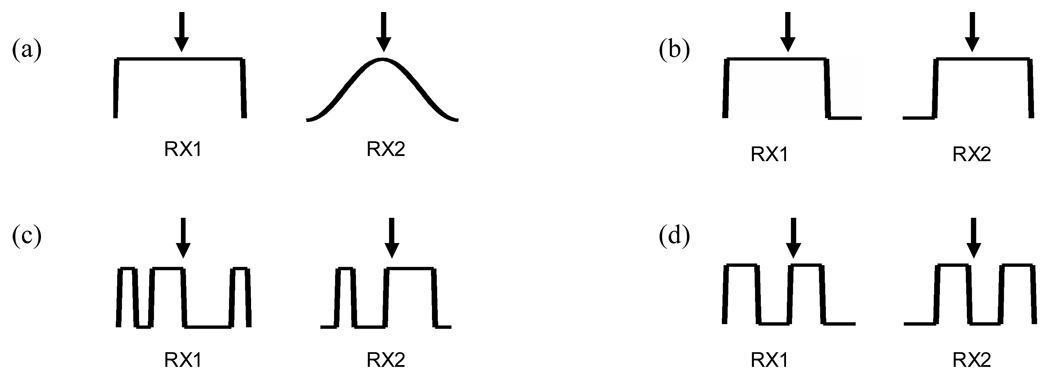
We can circumvent this trade-off between mainlobe width and sidelobe level, by axially cross-correlating segments of RF data from the two data sets obtained using these two apodization methods. The RF signals in the sidelobes of the beamformed point target image of these two data sets are quite different, giving near zero or negative cross-correlation values. The cross-correlation coefficient at each image sample is calculated. After thresholding, this matrix becomes the weighting matrix which can be multiplied to the combined RF data at each sample. Fig. 3 (a) shows two apertures where the first receive aperture has a uniform weighting, and where the second receive aperture has a Hanning apodization.

Fig. 3.

All algorithms use a common uniform transmit aperture. The lateral location of the focus is marked with the arrow. The interelement distance, or pitch, is one wavelength. Four pairs of receive apertures used with DAX, (a) Uniform and Hanning, (b) Common midpoint, (c) Random, and (d) Alternating pattern

B. Apodization Scheme 2: Common midpoint

Borrowing concepts from common midpoint apertures [9, 10], spatial compounding [11–13] and the translating apertures algorithm [14], the next pair of apodization functions to be investigated is two uniformly weighted apertures that have a fractional translation of the active subaperture. The speckle patterns obtained from the two apertures with a large number of common elements are still well correlated. This cross-correlation will decrease in the clutter region due to a steering of the sidelobes in opposite directions. The degree of steering or the amount of decorrelation will depend on the number of elements translated.

This design is demonstrated first using a simple 1 × 8 linear array shown in Fig. 3 (b). The main idea is that an equal amount of steering in opposite directions is purposely introduced. With a desired focused subaperture of 8 elements, only the first 6 elements or from channel 1 to 6 are activated for the first data set. This first image is a steered version of the standard beamformed image. Then, another set of data is acquired using the latter 6 elements, or from channel 3 to 8. The second image will also be a steered version of the standard beamformed image. The mainlobes will still be well cross-correlated with each other, but the sidelobes and the clutter portions are less correlated with each other. By calculating the cross-correlation coefficient at each image sample, this matrix becomes the “weighting factor” which can be multiplied to the minimum of the two images. For the simulation and experiment, we used a 64 element subaperture with an 8 element translation. With an 8 element translation or 14 % translation, we expect the speckle correlation obtained from the two apertures to be roughly 0.98 [13]. However, in the cystic region dominated by clutter and sidelobes, we expect the cross-correlation to be lower.

C. Apodization Scheme 3: Randomly selected aperture

In this scheme, by randomly selecting the two receive apertures with no common elements, a similar mainlobe with quite different clutter can be obtained. Since the two receive apertures are sparse, high clutter levels are expected where the amplitude of the clutter will depend on the sparseness of each aperture [15]. For the purpose of this paper, four different permutations were done in a point target simulation and the best random sparse aperture in terms of beamwidths and sidelobe level was chosen for subsequent cyst simulations and experiments. In Fig. 3 (c), a simple 1 × 8 linear array is used to demonstrate the two receive apertures. Four random elements are selected to receive for the first data set. Then for the second data set, unused elements from the first case are used. The cross-correlation coefficient at each image sample is calculated to generate a matrix and this matrix becomes the weighting factor. This is multiplied to the sum of the two images which is the standard beamformed image with uniform receive apodization.

D. Apodization Scheme 4: Alternating

In this scheme, the first receive aperture has alternating elements enabled. The second receive aperture will use the alternating elements that are not used in the first receive aperture. With these two apodizations, we purposely create grating lobes which are 180 degrees out of phase with each other. Then, by using cross-correlation we can distinguish between signals coming from a mainlobe and clutter signals. In our current scheme, signals with cross-correlation coefficients less than .001 are multiplied by .001 or reduced by 60 dB. Echoes with higher cross-correlation coefficients have more mainlobe signal and are multiplied by the cross-correlation coefficient.

Fig. 3 (d) is an illustration of a pair of receive apertures with a pitch of one wavelength λ. RX1 uses an alternating pattern of 2 elements on, 2 elements off. RX2 uses the opposite alternating pattern of 2 elements off, 2 elements on. These receive apertures are essentially sparse arrays with a four wavelength pitch. Thus, grating lobes are expected to be present in the PSF. The location of the nth grating lobe is given by

$${\theta }_n={\text{sin}}^{-1}\left(\frac{n\lambda }{d}\right)$$ (3)

where n is the nth grating lobe, λ is the ultrasound wavelength, and d is the interelement distance or pitch. The cross-correlation coefficient at each image sample is calculated to generate a matrix, and this matrix becomes the weighting factor. By summing data from these two receive apertures, we get the same data as from a uniformly weighted receive aperture. This RF data will then be weighted by the cross-correlation matrix. Instead of a 2-element alternating pattern as shown, any N-element alternating pattern can be used where N is less than half of the number of elements in the subaperture. The main difference between these configurations will be the location of the grating lobe. Increasing N will move the grating lobes closer to the mainlobe.

II. METHODS

We have performed computer simulations using Field II to generate lateral beamplots for all four designs [16]. A 5 MHz Gaussian pulse with 50 % bandwidth was used as the transmit pulse and a delta function as the element impulse response. For a point target simulation, an RMS energy value was calculated from the received voltage trace. All RMS energy values were converted to decibels after normalizing to the maximum energy level. The transmit and receive focus was fixed at 30 mm for the point target simulation. Since there is rarely a point target in a clinical environment, we have also done a simulation using a cylindrical 3 mm diameter anechoic cyst located at 30 mm depth embedded in a 3-D phantom of scatterers. The parameters for the simulation are listed in Table 1.

Table 1.

1 × 128 Linear Array and Imaging Parameters

Parameter	Value
Number of elements in subaperture	64
Center Frequency	5 MHz
Bandwidth	50 %
Azimuthal element Pitch	308 µm
Elevation Element Height	5 mm
Sound speed	1540 m/s
Transmit Focus	30 mm
Lateral beam spacing (beamplot simulation)	30 um
Lateral beam spacing (cyst)	150 um
Receive focal delay step (cyst)	0.1 mm

For our experimental setup, individual element RF signals were collected for off-line processing from an ATS spherical lesion phantom (ATS laboratories, Bridgeport, CT, Model 549) containing a 3 mm anechoic cyst using an Ultrasonix Sonix RP ultrasound system (Ultrasonix Medical Corporation, Richmond, BC, Canada) having 40 MHz sampling frequency. This system has great flexibility allowing the researcher to control parameters such as transmit aperture size, transmit frequency, receive aperture, filtering, and Time-Gain Compensation. In this experiment, a 128-element, 300 µm pitch, L14-5/38 linear array was used. A 1-cycle transmit pulse of 5 MHz and an f-number = 1.5 was used. In receive, element data was collected and receive beamforming was done off-line using Matlab (The MathWorks, Inc. Natick, MA). Dynamic receive focusing was used with focal updates every 0.1 mm. The image line spacing is 150 µm. Data from each channel was collected 32 times and averaged to minimize effects of electronic noise.

In an experimental setting as describe above, an analog RF signal is digitized with a sampling frequency of 40–60 MHz. Additional simulations were done with 40 MHz delay quantization in transmit and receive beamforming to model our experimental setup. This introduces delay quantization error and gives us a better understanding of how DAX performs on a commercially available system.

All signals in the experiments are bandpass filtered using a 63-tap finite impulse response (FIR) bandpass filter with frequency range limited to the −6 dB bandwidth of the transducer. After the signals are bandpass filtered, delayed, apodized and summed to create RX1 and RX2, the two sets of data are cross-correlated. The cross-correlation value is sent to a thresholding operator. If the value is less than or equal to ε, or 0.001 in our case, then the value is replaced with 0.001. If it is greater than 0.001, then the value remains unchanged. A second filter, which has the same passband window as the first filter, might be required to reduce sharp discontinuities in images that might be caused by multiplication of the weighting matrix. The Hilbert transform is used for envelope detection, and all images are displayed on a log scale.

IV. RESULTS

A. Point target simulation

Fig. 4 shows simulated lateral beamplots using Field II of a standard transmit/receive beam with uniform weighting compared to the four DAX schemes. The beamplots of all four methods have mainlobe widths basically equal to the mainlobe of the uniform apodization. At the same time, clutter near the mainlobe has dropped dramatically down to below −100 dB for all four methods. The −6, −20, −40, and −60 dB beamwidths are listed in Table 2. The −6 and −20 dB beamwidths are similar for all cases. For the uniform-Hanning and common midpoint schemes, the −6 dB beamwidths are 0.40 and 0.35 respectively or 11 % and 24 % smaller compared to the standard beamformed case. For the uniform-Hanning case, only portions of the two mainlobes are well correlated. For the common midpoint scheme, the two beams are steered and the overlap of the two beams is smaller than in random or alternating pattern schemes. Thus, having a cross-correlation value of slightly less than 1 and by multiplying this value by the minimum of the two data sets, the mainlobe width or the −6 dB beamwidth is narrower than in standard beamformed case. The −40 dB and − 60 dB widths are also narrowest for uniform-Hanning and common midpoint schemes. The −6 dB beamwidths for the randomly selected aperture and the alternating pattern are the same as the beamwidth for the case of standard beamforming.

Table 2.

Comparison of Beamwidths and Clutter Levels of the four designs

	Standard	Uniform-Hanning	Common midpoint	Randomly selected	Alternating pattern
− 6 dB (mm)	0.46	0.40	0.35	0.46	0.45
− 20 dB (mm)	0.80	0.89	0.79	0.81	0.79
−40 dB (mm)	2.67	0.99	1.00	1.89	2.05
−60 dB (mm)	8.58	1.08	1.92	2.12	2.20
Residual sidelobes	Clutter	<−80	<−60	<−60	<−100

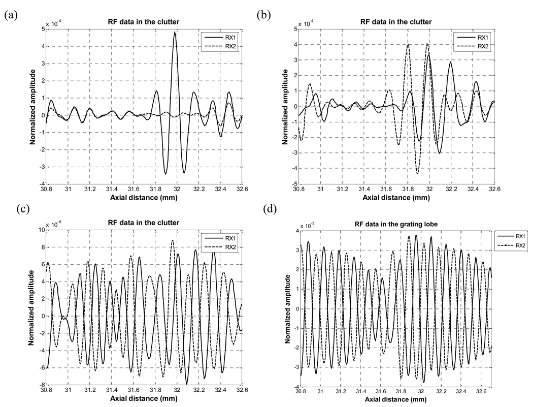
Fig. 5 shows the RF data inside the clutter and grating lobe regions for RX1 and RX2 for the four DAX schemes. It is interesting to note the effect of different apodizations on the clutter and grating lobe regions. For the uniform-Hanning apodization scheme, we see the amplitude of a Hanning apodized receive aperture is about 30 dB lower than the amplitude of a uniformly apodized receive aperture. With the common midpoint scheme, the two RF data are shifted by about 1 wavelength with respect to each other. In the randomly selected aperture scheme, the two data are “mirrored” versions of each other giving a 180° phase shift approximately. In the alternating pattern scheme, we also clearly see the two grating lobe regions are basically 180° out of phase with respect to each other. Although perhaps counterintuitive, using a larger alternating pattern can result in a better beam with DAX since the grating lobes here are beneficial since they narrow the beam particularly down at the −40 to −60 dB level. Cross-correlating these two signals would yield a cross-correlation coefficient near −1 and therefore a reduction of 60 dB in magnitude. The weighting matrix will be applied to the sum of these data sets.

Fig. 5.

RF data in the clutter region of a) Uniform-Hanning scheme b) Common midpoint scheme c) Randomly selected aperture scheme and d) Alternating pattern scheme.

B. Cyst simulation

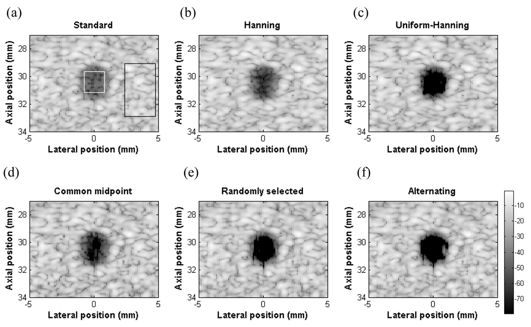
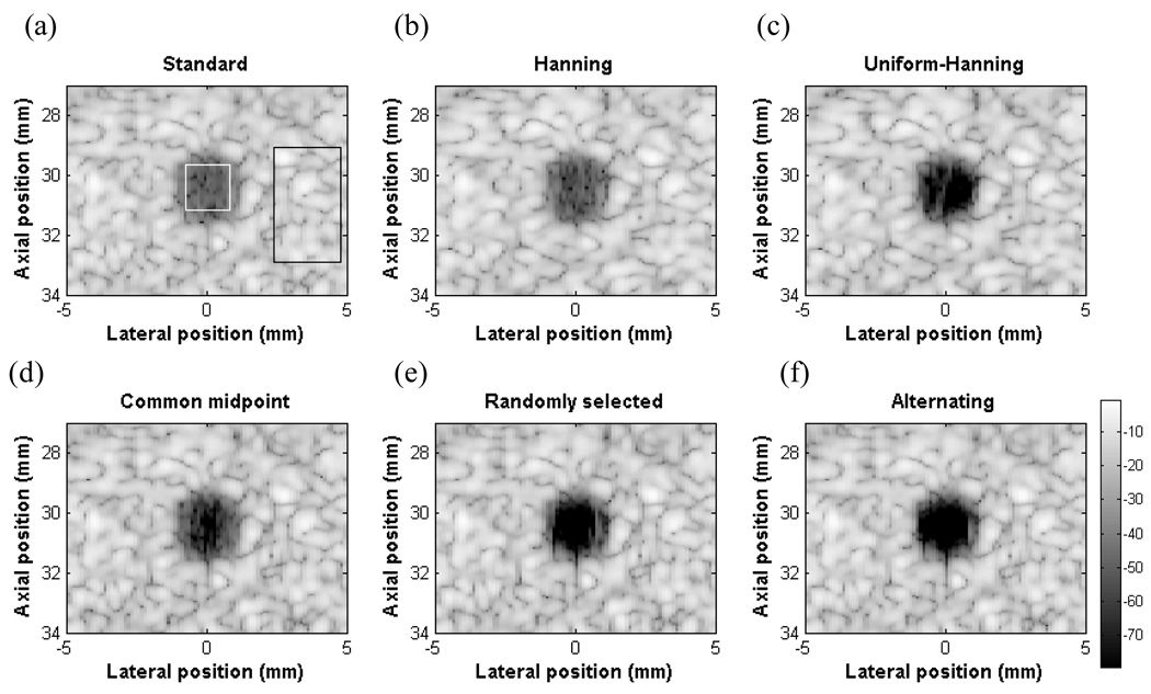
It is important to remember that the proposed algorithms are spatially varying and target-dependent. Therefore, although beamplots or PSFs are more intuitive, they are not exactly indicative of imaging performance for diffuse scatterers such as biological tissue. To further test the performance of these algorithms, Fig. 6 shows simulated images of a 3 mm diameter anechoic cyst with standard beamforming with uniform apodization, Hanning apodization and the four DAX schemes. To quantify improvement, the CNR for each of the images was calculated. CNR is defined as the difference between the mean of the background and the cyst in dB divided by the standard deviation of the background in dB [17],

$$\mathit{\text{CNR}}=\frac{\overline{S_t}-\overline{S_b}}{{\sigma }_b}$$ (7)

where $\overline{S_t}$ is the mean of the target, $\overline{S_b}$ is the mean of the background and σ_bis the standard deviation of the background. Signals coming from the speckle region are dominated by the mainlobe, thus giving a cross-correlation coefficient near 1. In the case of an anechoic cyst where the signal contribution from the mainlobe will be small, the sidelobes and grating lobes will be dominant giving a very low or negative cross-correlation value. The CNRs for the six images are 5.24, 6.85, 12.62, 12.92, 7.44, and 11.28 for standard beamforming with uniform apodization, Hanning apodization, uniform-Hanning, common midpoint, randomly selected and alternating pattern respectively. Regions used to calculate CNR are shown in the white and black rectangles for the target and background respectively. The figures are shown with 80 dB dynamic range. Qualitatively, the cyst using uniform weighting is most difficult to see (Fig. 6 a). Using Hanning apodization, the cyst has a better contrast but the speckle size is larger due to a widened mainlobe (Fig. 6 b). Using DAX processing, the cyst becomes more visible without affecting the mainlobe resolution (Fig. 6 c–f). The uniform-Hanning approach shows a dark cyst with a well defined boundary. This approach gives the highest CNR when multiplying the cross-correlation matrix with Hanning apodized data. In fact, multiplying by the minimum of the two data sets lowered the CNR below 10. The common midpoint approach shows a darker cystic region but the left and right edges show clutter. The amplitude of the clutter region is around 60 dB below the peak signal in the image. The randomly selected aperture approach also shows a darker cyst with some clutter. The alternating pattern approach performs as well as uniform-Hanning apodization scheme. All of the DAX schemes create some dark “pits” in the speckle region due to the randomness of the speckle. Methods to reduce these artifacts will be discussed later.

Fig. 6.

Cyst simulations with an anechoic region of 3 mm in diameter (a) Standard beamforming with uniform apodization (b) Hanning apodization, (c) Uniform-Hanning (d) Common midpoint (e) Randomly selected (f) Alternating pattern. The CNR values are (a) 5.24, (b) 6.85 (c) 12.92, (d) 7.44, (e) 11.28, and (f) 12.62

C. Cyst experiment

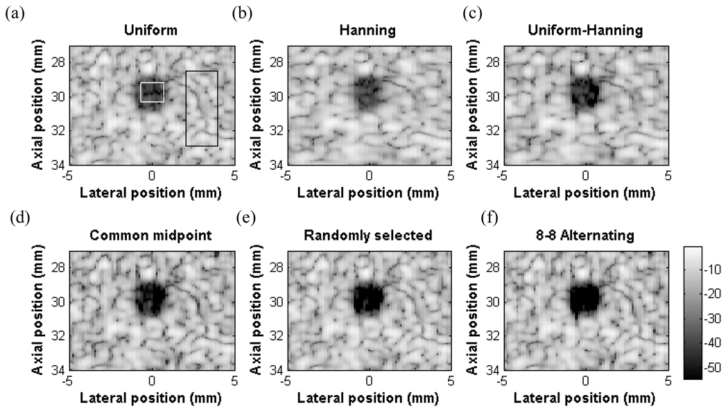
Fig. 7 shows the result from the cyst experiment using the Ultrasonix Sonix RP system and ATS tissue-mimicking phantom containing a 3 mm diameter anechoic cyst. The images are displayed with a 55 dB dynamic range after delay and sum beamforming, digital bandpass filtering, envelope detection and log-compression. The target region is marked with a white rectangle and the background region is marked with a black rectangle in the first image.

Fig. 7.

Experimental cyst images in a tissue-mimicking phantom. The cysts are 3 mm in diameter (a) Standard beamformed with uniform apodization (b) Hanning apodization (c) Uniform-Hanning (d) Common midpoint (e) Randomly selected (f) Alternating pattern. The CNR values are (a) 5.23, (b) 5.56, (c) 7.02, (d) 7.11, and (e) 11.39 (f) 11.64

Qualitatively, the cyst using standard beamforming with uniform apodization is the most difficult to see (Fig. 7 a). Using Hanning apodization, there is some improvement in CNR, and the speckle size is larger due to a widened mainlobe (Fig. 7 b). The uniform-Hanning, common midpoint, random all have some amount of “fill in”. The alternating pattern has the highest CNR at 11.64 compared to 5.23, 5.56, 7.02, 7.11, 11.39 for uniform, Hanning, uniform-Hanning, common midpoint, and random cases respectively. These CNR values are in very good agreement with the simulation results except for the Hanning apodization and uniform-Hanning scheme. This issue will be discussed in section D.

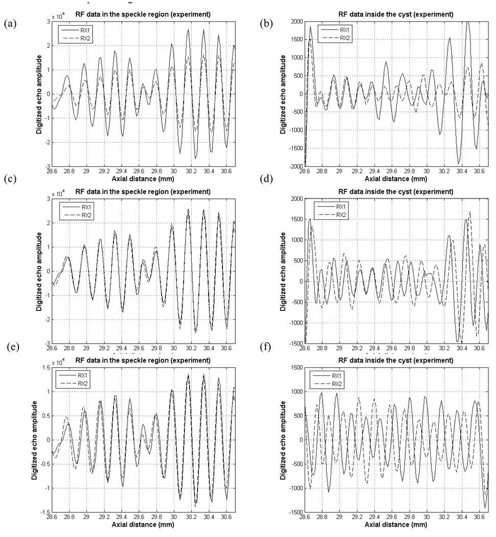
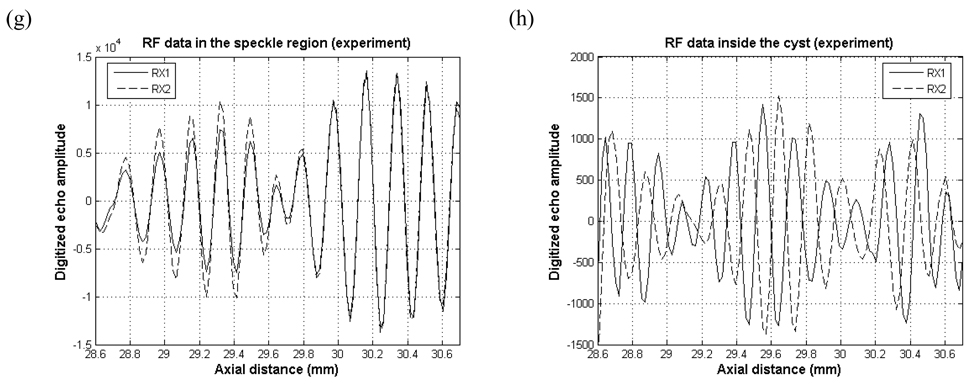
Fig. 8 shows experimental RF data from speckle region (left column) and inside the cyst (right column). In the speckle region, the waveforms from RX1 and RX2 are very similar yielding a cross-correlation coefficient near 1. For the cyst region, with uniform-Hanning scheme, the amplitude for Hanning apodized data (Fig. 8 b. RX2) is smaller than uniformly apodized data (Fig. 8 b. RX1). However, two sets of RF data are still correlated, and this fact does not agree with our point target and cyst simulation results. For the common midpoint scheme (Fig. 8 d), the two RF data are shifted relative to each other, but not as dramatically as in the simulation. For the randomly selected aperture (Fig. 8 f), and alternating pattern scheme (Fig. 8 h), the waveforms appear nearly 180° out of phase resulting in negative cross-correlation coefficients. Note that graphs in the left column of Fig. 8 are not on the same vertical scale as the graphs on the right column and that the echo magnitude inside the cyst is about 30 or 40 dB lower than the magnitude in the speckle region.

Fig. 8.

Experimental RF data in the speckle and cyst regions with (a), (b) Uniform-Hanning scheme (c), (d) common midpoint scheme (e), (f) randomly selected aperture scheme and (g), (h) alternating scheme

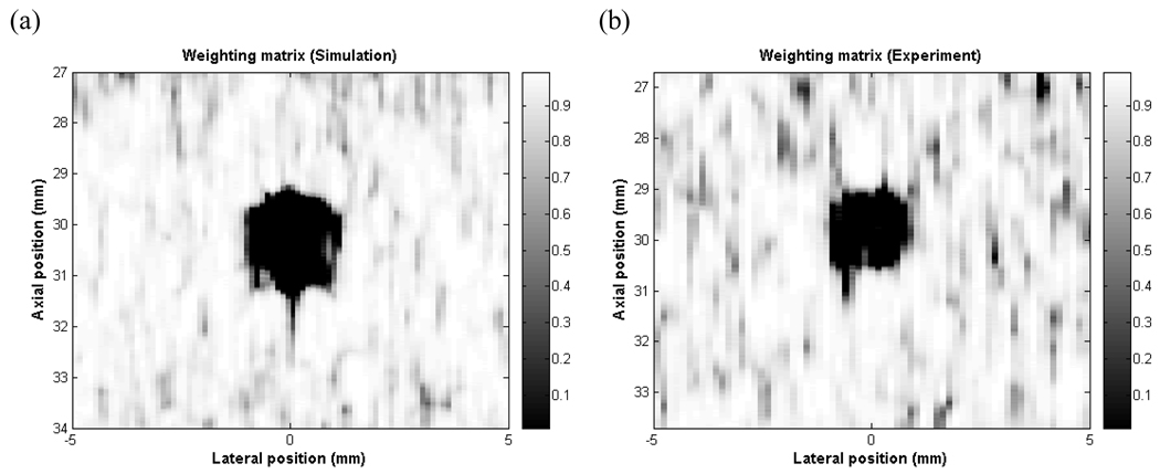
Fig. 9 shows the weighting matrices after the thresholding operation used for simulation and for the experiment using the DAX alternating pattern scheme. All cross-correlation values less than 0.001 were replaced with 0.001 to create the final weighting matrix. The cyst is clearly visible in the weighting matrix and the CNR values are 19.98 for simulation and 14.43 for experiment. Therefore, it may be possible to use these matrices as cross-correlation based images to locate a target, but this requires further investigation.

Fig. 9.

Weighting matrix used for DAX 8-8 alternating pattern in a) simulation, b) experiment in linear scale. Color bar shows the range of cross-correlation coefficients.

D. Simulation with 40 MHz quantization

The disparity between the CNRs of the simulated cyst and experimental cyst was further investigated with Field II simulations having 40 MHz quantization. The integrated lateral beamplots are shown in Fig. 10 and a cyst simulation with 40 MHz quantization is shown in Fig 11. Using standard beamforming with uniform apodization, the anechoic cyst still shows some “fill in” due to clutter. The CNRs are 5.39, 6.45, 10.45, 7.34, 11.03, 12.53 for standard beamforming, Hanning apodization, uniform-Hanning, common-midpoint, randomly selected and alternating pattern respectively. The effect of quantization is most prominent in the uniform-Hanning scheme. This can be explained considering quantization error as essentially a focusing error. In the other three apodization schemes, some or all elements in the receive aperture are different. Therefore if there are any focusing or quantization errors, each aperture sees different error contributions which are poorly correlated. However in the uniform-Hanning scheme, both apertures will be equally affected by any quantization errors introduced. These errors would be highly correlated. Table 3 summarizes the CNR values for two cyst simulations and experiment.

Fig. 10.

Lateral Beamplots comparing 4 DAX schemes with standard beamformed data with 40 MHz quantization. The standard beamformed PSF is compared with (a) uniform-Hanning scheme, (b) common midpoint scheme, (c) random scheme, and (d) the alternating pattern scheme.

Fig. 11.

Cyst simulation with 40 MHz quantization (a) Standard beamformed with uniform apodization (b) Hanning apodization (c) Uniform-Hanning (d) Common midpoint (e) Randomly selected (f) Alternating pattern. The CNR values are (a) 5.39, (b) 6.45, (c) 10.45, (d) 7.34, (e) 11.03 and (f) 12.53 respectively.

Table 3.

CNR values of the four designs

	Standard	Hanning	Uniform- Hanning	Common midpoint	Randomly selected	Alternating
CNR (simulation)	5.27	6.92	12.92	7.44	11.28	12.62
CNR (experiment)	5.23	5.56	7.02	7.11	11.39	11.64
CNR (simulation with 40 MHz quantization)	5.39	6.45	10.45	7.34	11.03	12.53

V. DISCUSSION AND FUTURE WORK

We have presented our Dual Apodization with Cross-correlation (DAX) technique that suppresses sidelobes and lowers clutter, thus improving CNR, without compromising spatial resolution in ultrasound imaging. The main idea behind this method is to use a pair of apodization schemes that are highly cross-correlated in the mainlobe but have low or negative cross-correlation in the sidelobe region. DAX uses two sets of beamformed data acquired with two different receive apertures and cross-correlates segments of RF data. This cross-correlation matrix serves as a pixel-by-pixel weighting function which will be multiplied to the minimum or to the sum of the two data sets. Theory and simulation were validated in ultrasound tissue-mimicking phantoms where contrast improvement in terms of CNR was 139 % in simulation and 123 % experimentally. Lateral and axial resolution are not sacrificed to improve CNR. The alternating pattern showed the highest CNR experimentally. This alternating pattern purposely creates two sets of grating lobes which are 180 ° out of phase with respect to each other. While grating lobes have long been a potential source for clutter in ultrasound imaging, DAX uses gratings lobes to help distinguish between mainlobe and clutter signals.

Occasionally, DAX will add artificial dark spots in the speckle region. In fact, the DAX algorithm slightly lowers the speckle SNR, defined as the ratio of mean to standard deviation of the scattered signal for fully developed speckle, by 4–11 %. The SNR in the speckle region before applying the DAX algorithm was 1.91. The SNR in the speckle region after the DAX algorithm was applied were 1.81, 1.70, 1.84 and 1.77 for Uniform-Hanning, Common midpoint, Random and Alternating pattern respectively. In cystic regions, it may be possible that clutter signals will have a high cross-correlation coefficient. In this situation, minimal or no improvement in contrast will be seen. The occurrence of both of these artifacts could be minimized by several straightforward options. Using a moving average or median filter on the cross-correlation coefficients is one approach. Since this process is a smoothing of the weighting matrix, the speckle pattern is not smeared. We have also briefly investigated the effect of correlation window on the cyst. A longer correlation window produced a poorly delineated cyst but with fewer dark spots in the speckle region. If the window size was too small, the speckle had more pits due to greater variation in cross-correlation coefficients. Empirically, 20–30 samples, which is roughly two wavelengths, performed best in terms of CNR. Lastly, the threshold and weighting as a function of ρ could be adjusted. All of these methods may help eliminate dark spots but may also lower CNR. This will be investigated in future work. Preliminary attempts with 1-D lateral cross-correlation gave us a slightly lower CNR than using 1-D axial cross-correlation. 2D cross-correlation gave us a comparable improvement to 1D axial cross-correlation but with increased computational load. This also requires further investigation.

One limitation of the current DAX algorithm is that it does not improve contrast of hyper-echoic or hypo-echoic lesions since signals are well-correlated inside and outside the lesions. A more generalized DAX algorithm which adjusts the weighting as a function of cross-correlation is under investigation to improve contrast of hyper–echoic or hypo-echoic targets. It is also interesting to note that the weighting matrix in Fig. 9 clearly identifies the cyst. This weighting matrix itself could possibly be used as a speckle free image. Additional work is needed to verify the feasibility of the cross-correlation based image for a variety of targets. Work is also underway to investigate the application of this technique to suppress sidelobes in other ultrasound technologies such as high frequency ultrasound, photoacoustic imaging, and 3-D ultrasound [18–20]. Also in future work, we will examine the robustness of this technique in the presence of low signal-to-noise ratios and aberrating layers. Lastly, we believe that DAX is relatively computationally inexpensive since a matrix of cross-correlation coefficients at only zero lag needs to be calculated on a 21-sample segment of RF data at 40 MHz sampling frequency. This would allow DAX to be easily implemented on a commercial real-time ultrasound system.

References

- 1.Bassett LW, Butler DL. Mammography and early breast cancer detection. American Family Physician. 1991;vol. 43:547–557. [PubMed] [Google Scholar]
- 2.Wu CM, Chen YC, Hsieh KS. Texture Features for Classification of Ultrasonic Liver Images. IEEE Trans. on Medical Imaging. 1992 June;vol. 11(no. 2) doi: 10.1109/42.141636. [DOI] [PubMed] [Google Scholar]
- 3.Lee F, Torp-Pedersen S, Litrup PJ. Hypoechoic lesions of the prostate: clinical relevance of tumor size, digital rectal examination, and prostate specific antigen. Radiology. 1989;vol. 170:29–32. doi: 10.1148/radiology.170.1.2462262. [DOI] [PubMed] [Google Scholar]
- 4.Guenther DA, Walker WF. Optimal Apodization Design for Medical Ultrasound Using Constrained Least Squares Part I: Theory. IEEE Trans. Ultras., Ferro., And Freq. Control. 2007 February;vol. 54:332–342. doi: 10.1109/tuffc.2007.247. [DOI] [PubMed] [Google Scholar]
- 5.Guenther DA, Walker WF. Optimal Apodization Design for Medical Ultrasound Using Constrained Least Squares Part II: Simulation Results. IEEE Trans. Ultras., Ferro., And Freq. Control. 2007 February;vol. 54:343–358. doi: 10.1109/tuffc.2007.248. [DOI] [PubMed] [Google Scholar]
- 6.Wang Hong. System and method for adaptive beamformer apodization. U.S. Patent No. 6436044. 2002 Aug.
- 7.Stankwitz HC, Dallaire RJ, Fienup JR. Nonlinear apodization for side lobe control in SAR imagery. IEEE Trans. Aerosp. Electron. Syst. 1995 Jan.vol. 31:23–52. [Google Scholar]
- 8.Harris FJ. On the use of windows for harmonic analysis with the discrete Fourier transform. Proceedings of the IEEE. 1978 Jan;vol. 66:51–83. [Google Scholar]
- 9.Haun MA, Jones DL, O’Brien WD. Overdetermined least-squares aberration estimates using common-midpoint signals. IEEE trans Medical imaging. 2004 Oct;23(1):1205–1220. doi: 10.1109/TMI.2004.831792. [DOI] [PubMed] [Google Scholar]
- 10.Li Y. Phase aberration correction using near-field signal redundancy. 1. Principles. IEEE Trans. Ultras., Ferro., And Freq. Control. 1997 March;vol. 44(2):355–371. doi: 10.1109/58.585120. [DOI] [PubMed] [Google Scholar]
- 11.Trahey GE, Smith SW, Von Ramm OT. Speckle pattern correlation with lateral aperture translation: Experimental results and implications for spatial compounding. IEEE Trans. Ultras., Ferro., And Freq. Control. 1986 May;vol. 33:257–264. doi: 10.1109/t-uffc.1986.26827. [DOI] [PubMed] [Google Scholar]
- 12.O'Donnell M, Silverstein SD. Optimum displacement for compound image generation in medical ultrasound. IEEE Trans. Ultras., Ferro., And Freq. Control. 1988 July;vol. 35:470–476. doi: 10.1109/58.4184. [DOI] [PubMed] [Google Scholar]
- 13.Dahl JJ, Guenther DA, Trahey GE. Adaptive Imaging and Spatial Compounding in the Presence of Aberration. IEEE Trans. Ultras., Ferro., And Freq. Control. 2005 July;vol. 52:1131–1144. doi: 10.1109/tuffc.2005.1503999. [DOI] [PubMed] [Google Scholar]
- 14.Walker WF. C- and D-Weighted Ultrasonic Imaging Using the Translating Apertures Algorithm. IEEE Trans. Ultras., Ferro., And Freq. Control. 2001 March;vol. 48:452–461. doi: 10.1109/58.911728. [DOI] [PubMed] [Google Scholar]
- 15.Davidsen RE, Jensen JA, Smith SW. Two-dimensional random arrays for real time volumetric imaging. Ultrason. Imag. 1994 Jul.vol. 16:143–163. doi: 10.1177/016173469401600301. [DOI] [PubMed] [Google Scholar]
- 16.Jensen JA, Svendsen JB. Calculation of pressure fields from arbitrarily shaped, apodized, and excited ultrasound transducers. IEEE Trans. Ultrason., Ferro. Freq. Contr. 1992;vol. 39:262–267. doi: 10.1109/58.139123. [DOI] [PubMed] [Google Scholar]
- 17.O'Donnell M, Flax SW. Phase-aberration correction using signals from point reflectors and diffuse scatterers: Measurements. IEEE Trans. Ultrason., Ferro.Freq. Contr. 1988;vol. 35(no. 6):768–774. doi: 10.1109/58.9334. [DOI] [PubMed] [Google Scholar]
- 18.Hu C-H, Cannata JM, Yen JT, Shung KK. Development of a real-time high frequency ultrasound digital beamformer for high frequency linear array transducers. IEEE Trans. Ultrason. Ferro.Freq. Control. 2006;53(2):317–323. doi: 10.1109/tuffc.2006.1593370. [DOI] [PubMed] [Google Scholar]
- 19.Bitton R, Zemp R, Li M-L, Yen JT. Photoacoustic Microscopy with a 30MHz Array and Receive System. 2006 IEEE Ultrasonics Symposium. 2006 Oct.:389–392. [Google Scholar]
- 20.Seo C, Yen JT. 64 × 64 2-D array transducer with row-column addressing. Ultrasonics Symposium, 2006 IEEE. 2006 Oct.:74–77. doi: 10.1109/TUFFC.2009.1107. [DOI] [PMC free article] [PubMed] [Google Scholar]