Evaluating uses of data mining techniques in propensity score estimation: a simulation study

SUMMARY

Background

In propensity score modeling, it is a standard practice to optimize the prediction of exposure status based on the covariate information. In a simulation study, we examined in what situations analyses based on various types of exposure propensity score (EPS) models using data mining techniques such as recursive partitioning (RP) and neural networks (NN) produce unbiased and/or efficient results.

Method

We simulated data for a hypothetical cohort study (n=2000) with a binary exposure/outcome and 10 binary/ continuous covariates with seven scenarios differing by non-linear and/or non-additive associations between exposure and covariates. EPS models used logistic regression (LR) (all possible main effects), RP1 (without pruning), RP2 (with pruning), and NN. We calculated c-statistics (C), standard errors (SE), and bias of exposure-effect estimates from outcome models for the PS-matched dataset.

Results

Data mining techniques yielded higher C than LR (mean: NN, 0.86; RPI, 0.79; RP2, 0.72; and LR, 0.76). SE tended to be greater in models with higher C. Overall bias was small for each strategy, although NN estimates tended to be the least biased. C was not correlated with the magnitude of bias (correlation coefficient [COR]=−0.3, p=0.1) but increased SE (COR=0.7, p<0.001).

Conclusions

Effect estimates from EPS models by simple LR were generally robust. NN models generally provided the least numerically biased estimates. C was not associated with the magnitude of bias but was with the increased SE.

BACKGROUND

The number of publications using propensity score methods has increased over the past several years.¹ Propensity score analysis^2,3 is appealing as a variable reduction technique in confounding adjustment, especially for pharmacoepidemiologic studies using claims databases that often have a number of covariates needed to be adjusted but have a few outcomes.⁴ Despite the increasing popularity of the method, relatively little is known about whether and in what situations the results of these techniques are more valid and/or efficient than those of traditional approaches⁵ and how exposure propensity score (EPS) models should be specified for maximizing the validity of results.

Over-fitting is not a concern when fitting EPS models, since good prediction of exposure status is the goal and not the interpretation of the individual regression coefficient of the EPS model.³ It has been recommended that the model be made as complex as possible with quadratic terms and/or interactions.⁶ In practice, investigators develop EPS models from a pool of statistical variables, sometimes including quadratic terms and/or higher-order interactions to represent potential confounding factors.⁵ The final set of variables is then chosen by stepwise procedures guided by statistical measures such as c-statistics, a non-parametric measure of model prediction.^7,8 Con-sequently, EPS models with very high c-statistics might be created. However, the effects of using EPS models with very high c-statistics on the validity and efficiency of the effect estimates in the subsequent outcome model adjusting for the EPS are not known.

Data mining techniques such as classification tree (recursive partitioning (RP) methods), and neural networks (NN) have been used in clinical epidemiology to create highly predictive models of clinical outcomes.^9,10 These techniques could be used in EPS modeling to produce predictive models with high c-statistics. Recently, some of these techniques were used in modeling propensity scores in applied medical and social sciences.^11–13 However, the situations in which the data mining techniques are useful for fitting EPS models leading to valid and efficient effect estimates have not been established.¹⁴

In the current simulation study, we examined whether and in what situations various EPS models using logistic regression (LR), RP, and NN produce unbiased and/or efficient results for measuring the effect of the exposure in the outcome model. We also examined whether model c-statistics predict bias and/or efficiency of the effect estimates in the outcome model.

METHOD

Overall simulation structure

We performed a set of Monte-Carlo simulation experiments. As in typical epidemiologic studies, the data were simulated for two hypothetical cohort studies (n=2000, and n=10 000) with a binary exposure A with p (A)=~0.5, a rare binary outcome Y with p (Y)=~0.02, and ten covariates (W_i, i 1…10). Four of W_i (i.e., W₁–W₄) were independently associated with both A and Y (confounders), three of W_i (i.e., W₅–W₇) were associated with the exposure only (exposure predictors), and three of W_i (i.e., W₈–W₁₀) were associated with the outcome only (outcome predictors) (Table 1). Six covariates (W₁, W₃, W₅, W₆, W₈, W₉) were binary in scale, whereas four (W₂, W₄, W₇, W₁₀) were continuous. Datasets were generated 1000 times for each of seven simulation scenarios.

Table 1.

Properties of 10 covariates and correlation matrix of the covariates

		Confounders				Exposure predictor			Outcome predictors
		W1	W2	W3	W4	W5	W6	W7	W8	W9	W10
Confounders	W 1	1
	W 2	0	1
	W 3	0	0	1
	W 4	0	0	0	1
Exposure predictors	W 5	0.2	0	0	0	1
	W 6	0	0.9	0	0	0	1
	W 7	0	0	0	0	0	0	1
Outcome predictors	W 8	0	0	0.2	0	0	0	0	1
	W 9	0	0	0	0.9	0	0	0	0	1
	W 10	0	0	0	0	0	0	0	0	0	1

Data generation

The data were generated in the following order according to the specified parameters:

• The covariates were generated in two steps. First, eight base covariates, (V_i, i=1…6, 8, 9) and two final covariates (W₇, W₁₀) were generated as independent standard normal random variables with zero mean and unit variance. Second, another final eight covariates (W_i, i=1…6, 8, 9) were modeled from V_i, i=1…6, 8, 9 as a linear combination of these variables. In the second step, correlations between some of the variables were introduced, with correlation coefficients varying from 0.2 to 0.9 (Table 1). These values refer the magnitude of correlation coefficient before dichotomizing some of the covariates (W₁, W₃, W₅, W₆, W₈, W₉). Dichotomizing these covariates would attenuate these values.

• The dichotomous exposure, A was modeled using LR as a function of W_i. The formula of the function (true propensity score) varied with scenarios (Appendix 1). First, R software generated a random number between 0 and 1 from a uniform distribution. A was set to be 1 if the randomly generated number was less than the estimated true propensity score (p [A ǀW_i]), and as 0 if the number was greater than the estimated true propensity score.

• The outcome, Y, was modeled using LR as a function of W_i and A (Appendix 1). Again, R software generated a random number between 0 and 1 from a uniform distribution. Y was set to be 1 if the randomly generated number was less than the probability of Y given A and W_i (p [Y ǀW_i, A]), and as 0 if the number was greater than the probability of Y given A and W_i.

In the simulation experiment, the effect of exposure was set to be constant with the coefficient of A=−0.4 (odds ratio of 0.67), which was based on the effect hormone replacement therapy on fracture or colorectal cancer.^15,16 The formulas of the data generation functions used in each scenario are in Appendix 1. The coefficients of the formulas are in Appendix 2, which were based on coefficients for claims data-based variables modeling use of statins.

Simulation scenarios

To compare the performance of different modeling/data mining techniques (LR,¹⁷ NN, and RP) and their usefulness in various situations, we based simulations on realistic scenarios that differed by the complexity of the associations between the exposure and the covariates. We considered seven scenarios (Scenario A–G), which varied with the degree of linearity and/or additivity of modeled associations between the exposure and the covariates (Table 2). These assumptions were incorporated into the structure of the true propensity score for each scenario (Appendix 1). The simplest scenario (Scenario A) assumed linear associations between continuous covariates and the exposure and additive effects for all covariates. We modeled moderate and mild non-linearity and non-additivity by varying the number of interaction terms (10 vs. 3) and the number of quadratic terms (3 vs. 1). We modeled a mildly complex association with three two-way interactions and/or one quadratic term involving the four confounders and a moderately complex association with 10 two-way interactions and/or three quadratic terms (Table 1, Appendix 1 and 2). The values for coefficients of these quadratic and interaction terms ranged from 30% to 100% of the values for the coefficients of the main effect terms (Appendix 2).

Table 2.

Description of seven scenarios (Scenario A–G) for data generation

	Additive (main effects only)	Mild non-additivity (three two-way interaction terms involving confounders)	Moderate non-additivity (10 two-way interaction terms involving confounders)
Linear (main effects only)	A	D	F
Mild non-linearity (one quadratic term)	B	E	–
Moderate non-linearity (three quadratic terms)	C	–	G

In practice, researchers modeling EPS do not know the true structure of association between exposure and the covariate. As a consequence, they might create a misspecified EPS model that is too simple by falsely assuming linear and/or additive relationships between covariates and the exposure or a misspecified model that is too complex. For example, ignoring potential interactions in specifying EPS model might bias the effect estimates. We hypothesized that a simple LR model with only main effects would give an unbiased estimate only when associations between exposure and covariates are linear and additive (Scenario A), whereas EPS models developed by data mining techniques might give less unbiased estimates when the association between exposure and covariates becomes more complex (Scenario B–G).

Empirical exposure propensity score models

For each scenario, we compared different modeling strategies for EPS models: (1) NN with 1 layer and 10 hidden nodes, (2) RP without pruning (RP1), (3) RP with pruning (default setting in the R Software package with a cost complexity parameter of 0.01) (RP2), and (4) LR including only all possible main effects. When constructing trees in RP models, we produced a tree by executing the RP process as far as possible. (RP1). However, such a saturated tree is generally too big and prone to noise due to overfitting. We then took another step to prune the saturated tree in order to obtain a reasonably sized tree that is still discriminative but robust with respect to the noise. (RP2).

Measures of interests

The unconfounded effect of A on Y was estimated by matching subjects within 0.1 standard deviations of the empirical propensity score. The data generation process was repeated until all 1000 datasets for a given scenario had greater than 40 outcomes. The situation in which there were zero exposed or unexposed cases after matching was avoided by discarding datasets with less than 40 outcomes before matching.

In the matched dataset, the exposure effect was estimated from a LR outcome model:

$$\mathrm{Pr}[Y=1\mid A]={(1+\exp \{-({\gamma }_0+{\gamma }_{1}A)\left\}\right)}^{-1}$$

Since this model was fit on the subset of exposed (A=1) and non-exposure (A=0) subjects matched on the propensity score, the estimated exposure effect ${\widehat{\gamma }}_1$ reflects the effect of exposure conditional on the propen sity score. For each set of 1000 simulations, we calculated the average of the estimated effect measure, $\overline{{\widehat{\gamma }}_1}$.

We reported the bias (BIAS), the standard error (SE) from the outcome model, as well as the c-statistics (C) of EPS models for each scenario. BIAS was calculated by $\mid \overline{{\widehat{\gamma }}_1}-{\widehat{\gamma }}_1\mid$ where the γ₁ is the true effect of exposure, which was set to be −0.4 in the models that generated the outcome data. SE is an average standard error of ${\widehat{\gamma }}_1$ in each simulation. C is the average area under the receiver operating characteristics (ROC) curve calculated for each EPS model in each simulation.

To examine possible association between C and BIAS or SE, we also reported the correlation coefficient (COR) between C and these measures. COR_B is a correlation coefficient between C_MN and BIAS_MN, where M=methods of EPS (NN, RP1, RP2, or LR), and N=types of scenarios (scenario A–G). Similarly, COR_S is a correlation coefficient between C_MN and SE_MN.

Computation

We performed all simulations using R version 2.0.1 ^11,18,19 on a UNIX or Windows XP platform.

RESULTS

Small dataset (n=2000) simulation

Table 3 shows the characteristics of small (n=2000) dataset simulations before and after matching on propensity scores. Because all the datasets have 40 or more outcomes, the mean number of the outcome cases was greater than 40 but no datasets had zero exposed or non-exposed cases before or after matching. In the original datasets, the mean crude log odd ratios for the exposure ranged from −0.2 to 0.29, reflecting the amount of confounding in each dataset (unconfounded log odds ratio=−0.4). Matching reduced the size of the dataset to 50–60% of the original, and RP1 (RP without pruning) had the smallest dataset size.

Table 3.

Characteristics of simulation datasets

	Before matching				Matched (NNET)		Matched (RPART1)		Matched (RPART2)		Matched (LOGISTIC)
	Cases	Exposed cases	Crude LOG OR	Size of cohort	Cases	Size of cohort	Cases	Size of cohort	Cases	Size of cohort	Cases	Size of cohort
Scenario A
Minimum	40	9	−1.41	2000	15	984	10	1018	17	1198	15	1162
Mean	47.4	−21.7	0.21	2000	28.4	1179.0	26.6	1109	33.3	1389	30.8	1273
Maximum	71	36	0.80	2000	45	1366	44	1218	52	1566	51	1402
Secnario B
Minimum	40	8	−1.39	2000	17	1016	14	1006	21	1172	18	1148
Mean	48.1	19.4	−0.25	2000	28.9	1182	27.1	1094	33.2	1362	31.5	1283
Maximum	72	35	0.91	2000	45	1366	46	1218	52	1560	52	1418
Scenario C
Minimum	40	9	−1.49	2000	16	1020	14	926	18	1092	21	1286
Mean	47.6	20.9	−0.27	2000	29.1	1171	25.7	1030	32.2	1281	34.0	1403
Maximum	72	40	0.70	2000	46	1356	44	1130	50	1436	55	1546
Scenario D
Minimum	40	11	−1.15	2000	14	912	14	952	14	1138	17	1062
Mean	47.3	21.8	−0.22	2000	27.3	1107	26.0	1060	31.8	1316	28.8	1192
Maximum	71	36	0.90	2000	47	1258	45	1208	51	1486	46	1298
Scenario E
Minimum	40	9	−1.31	2000	14	920	13	954	17	1136	18	1086
Mean	48.0	19.6	−0.26	2000	28.1	1116	26.3	1057	32.2	1318	30.0	1208
Maximum	73	32	0.89	2000	44	1270	43	1162	53	1490	50	1336
Scenario F
Minimum	40	10	−1.42	2000	14	918	12	936	13	1088	15	1084
Mean	47.0	23.2	−0.22	2000	27.7	1118	25.9	1039	31.6	1276	29.6	1217
Maximum	71	39	0.59	2000	43	1252	47	1136	52	1498	48	1334
Scenario G
Minimum	40	9	−1.37	2000	14	948	12	910	19	1092	21	1200
Mean	47.2	22.3	−0.29	2000	28.3	1112	25.2	1000	32.0	1255	33.1	1330
Maximum	72	41	0.77	2000	47	1272	38	1106	50	1416	51	1478

Table 4 shows the average c-statistics (C) of EPS models, SE, and BIAS of the estimated effect of the exposure for Scenario A–G for the analysis using the data matched by the propensity score. C of EPS models developed by data mining techniques tended to be higher than that of LR models except for RP2 (RP with pruning). Mean C over scenarios were 0.86 for NN, 0.79 for RP1, 0.72 for RP2, and 0.76 for LR (Table 4a). Furthermore, as the modeled association between exposure and covariates became more complex, data mining techniques (NN, RP1, and RP2) tended to yield higher C. For example, the difference in C between the data with the least complex association (Scenario A) and those with the most complex association (Scenario G) was 0.03, 0.02, and 0.04 in NN, RP1, and RP2, respectively, whereas the difference in LR model with main effect only (LR) was −0.03. This probably reflects the ability of data mining techniques to specify the non-linear and non-additive associations between exposure and covariates correctly.

Table 4.

C-statistics, standard errors and bias of the estimated effect of A on Y in Scenario A–G (n=2000 datasets)

	EPS MODELS
	NN	RP1 (no pruning)	RP2 (pruning)	LR
(a) C-statistics
Scenario A	0.84	0.78	0.70	0.76
Scenario B	0.85	0.78	0.70	0.76
Scenario C	0.86	0.80	0.74	0.72
Scenario D	0.86	0.79	0.71	0.79
Scenario E	0.86	0.79	0.71	0.78
Scenario F	0.86	0.79	0.72	0.77
Scenario G	0.87	0.80	0.74	0.73
(b) Standard error of the estimates
Scenario A	0.40	0.41	0.36	0.38
Scenario B	0.40	0.41	0.36	0.38
Scenario C	0.40	0.42	0.37	0.36
Scenario D	0.41	0.42	0.37	0.39
Scenario E	0.40	0.42	0.37	0.39
Scenario F	0.40	0.42	0.38	0.39
Scenario G	0.40	0.42	0.38	0.37
(c) Bias of the estimates*
Scenario A	0.006 (2%)	0.014 (4%)	0.075 (19%)	0.008 (2%)
Scenario B	0.018 (5%)	0.011 (3%)	0.027 (7%)	0.026 (7%)
Scenario C	0.051 (13%)	0.052 (13%)	0.031 (8%)	0.038 (10%)
Scenario D	0.016 (4%)	0.018 (5%)	0.050 (13%)	0.020 (5%)
Scenario E	0.013 (3%)	0.036 (9%)	0.015 (4%)	0.031 (8%)
Scenario F	0.001 (<1%)	0.003 (<1%)	0.085 (21%)	0.025 (6%)
Scenario G	0.066 (17%)	0.002 (<1%)	0.021 (5%)	0.031 (8%)

NN: neural networks; RP1: recursive partitioning without pruning; RP2: recursive partitioning with pruning; LR: logistic regression with main effects.

^*Values in Table 4(c) represent absolute bias (% relative bias). The relative bias (%) was calculated by absolute bias/the true effect of the exposure times 100.

Reflecting the size of the dataset after matching for each EPS model, SEs of the estimates were largest in RP1 and then in NN (Table 4b). We expected that EPS models by data mining techniques would produce unbiased effect estimates when the association between the exposure and the covariates are non-linear and/or non-additive (Scenario B–G). We also expected that LR would produce biased estimates in Scenario B–G because LR included only main effects and cannot correctly specify the association with non-linearity and/or non-additivity. Overall, the magnitude of bias in the effect estimates for all EPS models was within 20% of the size of the effect estimates (Table 4c). Although the overall magnitude of the bias in LR was relatively small, the estimates by LR were least biased in Scenario A, and more biased in other scenarios (B–G). NN produced the least biased estimates except in Scenarios C and G. Because both scenarios have moderate non-linearity created by three quadratic terms in common, we investigated the possibility that the poor performance of NN may be due to the large coefficient of one of the quadratic terms (W₇×W₇) involving one of the independent covariates. To examine this, we eliminated this quadratic term and re-ran the simulations for Scenarios C and G (Table 5). In the new simulations for the modified Scenarios C and G, C and BIAS of the LR model were larger than those in the old simulations for original Scenarios C and G. However, NN had similar C and SE but a smaller bias. Overall, with the new Scenarios C and G, NN tended to produce the least biased estimates in Scenario B–G, but LR produced the least biased estimates in Scenario A.

Table 5.

C-statistics, standard errors, and bias of the estimated effect of A on Y in Scenario A, B, Modified C, D, E, F, and Modified G (n=2000 datasets)

	EPS MODELS
	NN	RP1 (no pruning)	RP2 (pruning)	LR
(a) C-statistics
Scenario A	0.84	0.78	0.70	0.76
Scenario B	0.85	0.78	0.70	0.76
Scenario C	0.83	0.78	0.69	0.75
Scenario D	0.86	0.79	0.71	0.79
Scenario E	0.86	0.79	0.71	0.78
Scenario F	0.86	0.79	0.72	0.77
Scenario G	0.86	0.79	0.79	0.75
(b) Standard error of the estimates
Scenario A	0.40	0.41	0.36	0.38
Scenario B	0.40	0.41	0.36	0.38
Scenario C	0.40	0.42	0.38	0.38
Scenario D	0.41	0.42	0.37	0.39
Scenario E	0.40	0.42	0.37	0.39
Scenario F	0.40	0.42	0.38	0.39
Scenario G	0.39	0.42	0.41	0.38
(c) Bias of the estimates*
Scenario A	0.006 (2%)	0.014 (4%)	0.075 (19%)	0.008 (2%)
Scenario B	0.018 (5%)	0.011 (3%)	0.027 (7%)	0.026 (7%)
Scenario C	0.019 (5%)	0.055 (14%)	0.012 (3%)	0.061 (15%)
Scenario D	0.016 (4%)	0.018 (5%)	0.050 (13%)	0.020 (5%)
Scenario E	0.013 (3%)	0.036 (9%)	0.015 (4%)	0.031 (8%)
Scenario F	0.001 (<1%)	0.003 (<1%)	0.085 (21%)	0.025 (6%)
Scenario G	0.029 (7%)	0.032 (8%)	0.002 (<1%)	0.062 (16%)

NN: neural networks; RP1: recursive partitioning without pruning; RP2: recursive partitioning with pruning; LR: logistic regression with main effects.

Values in Table 5(c) represent absolute bias (% relative bias). The relative bias (%) was calculated by absolute bias/the true effect of the exposure times 100.

Finally, we plotted C on the x-axis and BIAS or SE on the y-axis across all scenarios and different modeling strategies in Figures 1 and 2. C-statistics were not correlated with the magnitude of bias in the effect estimates (COR_B=−0.29, p=0.13) but were correlated with increased SE (COR_S=0.71, p<0.001). The finding that higher c-statistic leads to larger SE is not surprising but rather expected because a c-statistic near 1.0 would make the model unstable and increase SE of the effect estimate to infinite.

Figure 1.

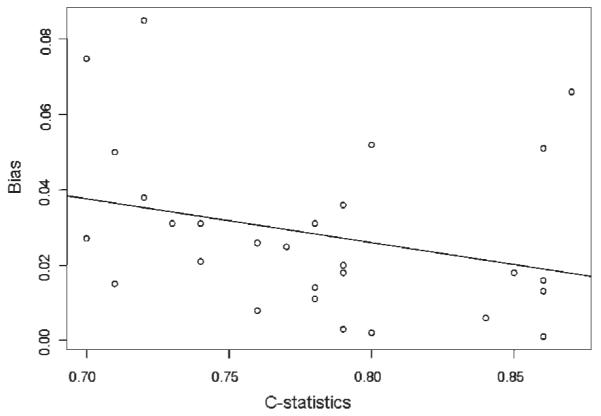
Correlation between C-statistics and Bias of the effect estimates of the exposure

Figure 2.

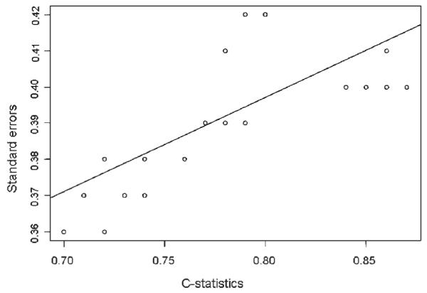
Correlation between C-statistics and standard errors of the effect estimates of the exposure

This correlation was implied by the sizes of the matched datasets because the models with large C discriminate the exposed and unexposed by the propensity scores and therefore have less overlap for matching.

Large dataset (n=10 000) simulation

In the large dataset simulations, we increased the size of the data to n=10 000 using the same scenarios except that we used the modified Scenarios C and G. (results in Table 6) The C of the EPS models by data mining techniques tended to be smaller than those in small datasets, reflecting the production of less overfitting models in larger datasets by these techniques. Because the datasets were much larger, SE of the estimates were smaller but kept the same trend among the models. For all EPS models, the biases were smaller than in small dataset simulations, and NN and RP1 tended to produce relatively less biased estimates in many scenarios.

Table 6.

C-statistics, standard errors, and bias of the estimated effect of A on Y in Scenario A, B, Modified C, D, E, F, and Modified G (n=10 000 datasets)

	EPS MODELS
	NN	RP1 (no pruning)	RP2 (pruning)	LR
(a) C-statistics
Scenario A	0.77	0.79	0.67	0.76
Scenario B	0.78	0.79	0.66	0.75
Scenario C	0.78	0.80	0.66	0.74
Scenario D	0.80	0.81	0.69	0.78
Scenario E	0.80	0.81	0.68	0.78
Scenario F	0.80	0.81	0.70	0.77
Scenario G	0.80	0.81	0.70	0.75
(b) Standard error of the estimates
Scenario A	0.17	0.18	0.16	0.17
Scenario B	0.17	0.18	0.16	0.17
Scenario C	0.18	0.19	0.16	0.17
Scenario D	0.18	0.19	0.16	0.17
Scenario E	0.17	0.19	0.16	0.17
Scenario F	0.17	0.19	0.16	0.17
Scenario G	0.17	0.19	0.16	0.17
(c) Bias of the estimates*
Scenario A	0.011 (3%)	0.003 (1%)	0.107 (27%)	0.021 (5%)
Scenario B	0.011 (4%)	0.017 (4%)	0.060 (15%)	0.006 (2%)
Scenario C	0.011 (2%)	0.033 (8%)	0.006 (2%)	0.016 (4%)
Scenario D	0.011 (2%)	0.010 (3%)	0.081 (20%)	0.011 (3%)
Scenario E	0.011 (1%)	0.002 (<1%)	0.043 (11%)	0.025 (6%)
Scenario F	0.011 (4%)	0.005 (1%)	0.110 (28%)	0.011 (3%)
Scenario G	0.011 (3%)	0.017 (4%)	0.043 (11%)	0.044 (11%)

NN: neural networks; RP1: recursive partitioning without pruning; RP2: recursive partitioning with pruning; LR: logistic regression with main effects.

Values in Table 6(c) represent absolute bias (% relative bias).The relative bias (%) was calculated by absolute bias/the true effect of the exposure times 100.

DISCUSSION

In our simulation study, data mining techniques tended to yield higher C for the EPS models than LR, except for RP with pruning. SEs of the effect estimates were greater in models with high C, since an EPS model with high C creates less overlap in propensity scores and therefore results in a smaller size of the matched dataset. Overall, NN tended to produce the least biased estimates in many scenarios with non-additivity and/ or non-linearity when the datasets were small or large. This tendency in NN was not enhanced in the simulation using datasets with only confounders. However, the magnitude of bias in the effect estimates was relatively small in all models and the bias in LR was not substantial even in the scenarios with non-linearity and/or non-additivity.

A previous simulation study examining variable selection in EPS models showed that higher C was associated with higher SE in the effect estimates,²⁰ which was also seen in our simulation study. Although maximizing C is commonly used as guide to creating an optimal EPS model, one should be cautious about the possibility that EPS models with a higher C might result in lower precision in the effect estimates. The validity and appropriateness of a propensity score should not be judged by the size of C.

In practice, researchers using modeling propensity score usually do not know the true structure of the association between the exposure and the covariate. It has been reported that misspecification of propensity score models introduces less bias than does misspecification of multivariate logistic outcome models.^21,22 In our stimulation study, although the magnitude of bias in LR (misspecified model for Scenario B–G) was not large, LR tended to produce more biased estimates than NN in Scenario B–G. This suggests that NN has the ability to correctly detect the associations between the exposure and the covariates. Our simulations also suggest that NN might have created a misspecified propensity score model by adding unnecessary complexity for some scenarios. Nonetheless, LR models with main effects only demonstrated a robust performance by its small bias.

The usefulness of RP and the use of pruning should be interpreted with caution. The EPS model by RP without pruning had the highest SE. The RP with pruning tended to produce relatively biased estimates. We used the default setting of R to set the cost complexity parameter for pruning, which might have produced trees that were too small and had very low discrimination for the exposure. Further studies are required to assess the usefulness of RP with appropriate amounts of pruning.

The results of our simulation study might be limited in situations not represented by our simulated data. However, we modeled the situations typical in pharmacoepidemiologic studies, such as large number of observations, a rare outcome, a common exposure, and a moderate effect of the exposure. The coefficients of the data generation model were based on coefficients of the actual claims data modeling propensity of statin use. In fact, it is one of the strengths of our study that the ranges of variables used in simulations were consistent with the expected ranges in the actual pharmacoepidemiology practice. We also introduced colinearity of the covariates in the data, which may be common in pharmacoepidemiologic studies.

In our simulation studies of realistic but limited scenarios, the models created by NN had the least biased estimates in many scenarios. However, effect estimates from EPS models by simple LR approach were robust to misspecification of EPS model structure, and no single method was universally better than the others. C-statistics, a measure often used as a guide for modeling EPS, were not associated with the magnitude of bias but were associated with increased SEs of the estimates. Further studies are needed to assess the usefulness of data mining techniques in a broader range of realistic scenarios.

KEY POINTS.

• Data mining techniques can be used and might offer some advantage in estimating PS.

• PS models created by neural networks had the least biased estimates in many scenarios in our stimulation study.

• PS models using logistic regression was robust to misspecification of the model structure.

• C-statistics were not associated with amount of bias but were associated with increased SE, and not recommended to be used to guide PS model selection.

• Further studies are needed using a broader range of realistic scenarios and real data.

APPENDIX 1. DATA GENERATION MODEL FORMULAS

True propensity score models

Scenario A (a model with additivity and linearity)

Pr [A = 1ǀW_i] (1+exp{−(β₀ +ǀβ₁W₁+β₂W₂+ β₃W₃+ β₄W₄+β₅W₅+β₆W₆+β₇W₇)})⁻¹

Scenario B (a model with mild non-linearity)

Pr [A=1ǀW_i]=(1+exp{−(β₀+β₁W₁+β₂W₂+β₃W₃+ β₄W₄+β₅W₅+β₆W₆+β₇W₇+β₂W₂W₂})⁻¹

ScenarioC(amodelwithmoderatenon-linearity)

Pr [A=1ǀW_i]=(1+exp{−(β₀+β₁W₁+β₂W₂+β₃W₃+ β₄W₄+β₅W₅+β₆W₆+β₇W₇+β₂W₂W₂+β₄W₄W₄+β₇W₇W₇)})⁻¹

Scenario D (a model with mild non-additivity)

Pr [A=1ǀW_i]=(1+exp{−(β₀+β₁W₁+β₂W₂+β₃W₃+ β₄W₄+β₅W₅+β₆W₆+β₇W₇+β₁×0.5×W₁W₃+β₂×0.7×W₂W₄+β₄×0.5×W₄W₅+β₅×0.5×W₅W₆)})⁻¹

Scenario E (a model with mild non-additivity and non-linearity)

Pr [A=1ǀW_i]=(1+exp{−(β₀+β₁W₁+ β₂W₂+β₃W₃+ β₄W₄+β₅W₅+β₆W₆+β₇W₇+β₂W₂W₂+β₁×0.5×W₁W₃+β₂×0.7×W₂W₄+β₄×0.5× W₄W₅+β₅×0.5×W₅W₆)})⁻¹

Scenario F (a model with moderate non-additivity)

Pr [A=1ǀW_i]=(1+exp{−(β₀+β₁W₁+β₂W₂+β₃W₃+ β₄W₄+β₅W₅+β₆W₆+β₇W₇+β₁×0.5×W₁W₃+β₂×0.7×W₂W₄+β₃×0.5×W₃W₅+β₄×0.7×W₄W₆+ β₅×0.5×W₅W₇+β₁×0.5×W₁W₆+β₂×0.7×W₂W₃+β₄×0.5×W₄W₅+β₅×0.5× W₅W₆)})⁻¹

Scenario G (a model with moderate non-additivity and non-linearity)

Pr [A=1ǀW_i]=(1+exp{−(β₀+ β₁W₁+β₂W₂+β₃W₃+β₄W₄+β₅W₅+β₆W₆+β₇W₇+β₂W₂W₂+β₄W₄W₄+β₇W₇W₇+β₁×0.5×W₁W₃+ β₂×0.7×W₂W₄+β₃×0.5×W₃W₅+β₄×0.7×W₄W₆+β₅×0.5×W₅W₇+β₁×0.5×W₁W₆+β₂×0.7× W₂W₃+β₃×0.5×W₃W₄+β₄×0.5×W₄W₅+β₅×0.5×W₅W₆)})⁻¹

Outcome model

Scenario A–G

Pr [Y=1ǀA, W_i]=(1+exp{−(α₀+α₁W₁+α₂W₂+α₃W₃+α₄W₄+α₅W₈+α₆W₉+α₇W₁₀+ γ₁A)})⁻¹

APPENDIX 2. COEFFICIENTS FOR DATA GENERATION MODELS

β₀=0

β₁=0.8

β₂=−0.25

β₃=0.6

β₄=−0.4

β₅=−0.8

β₆=−0.5

β₇=0.7

α₀=−3.85

α₁=0.3

α₂=−0.36

α₃=−0.73

α₄=−0.2

α₅=0.71

α₆=−0.19

α₇=0.26

γ₁=−0.4

REFERENCES

- 1.Sturmer T, Joshi M, Glynn RJ, Avorn J, Rothman KJ, Schneeweiss S. A review of the application of propensity score methods yielded increasing use, advantages in specific settings, but not substantially different estimates compared with conventional multivariable methods. J Clin Epidemiol. 2006;59(5):437–447. doi: 10.1016/j.jclinepi.2005.07.004. [DOI] [PMC free article] [PubMed] [Google Scholar]
- 2.Rosenbaum PR, Rubin DB. The central role of the propensity score in observational studies for causal effects. Biometrika. 1983;70:41–55. [Google Scholar]
- 3.Rubin DB. Estimating causal effects from large data sets using propensity scores. Ann Intern Med. 1997;127(8 Pt 2):757–763. doi: 10.7326/0003-4819-127-8_part_2-199710151-00064. [DOI] [PubMed] [Google Scholar]
- 4.Austin PC, Mamdani MM, Stukel TA, Anderson GM, Tu JV. The use of the propensity score for estimating treatment effects: administrative versus clinical data. Stat Med. 2005;24(10):1563–1578. doi: 10.1002/sim.2053. [DOI] [PubMed] [Google Scholar]
- 5.Shah BR, Laupacis A, Hux JE, Austin PC. Propensity score methods gave similar results to traditional regression modeling in observational studies: a systematic review. J Clin Epidemiol. 2005;58(6):550–559. doi: 10.1016/j.jclinepi.2004.10.016. [DOI] [PubMed] [Google Scholar]
- 6.D’Agostino RB., Jr Propensity score methods for bias reduction in the comparison of a treatment to a non-randomized control group. Stat Med. 1998;17(19):2265–2281. doi: 10.1002/(sici)1097-0258(19981015)17:19<2265::aid-sim918>3.0.co;2-b. [DOI] [PubMed] [Google Scholar]
- 7.Stone RA, Obrosky DS, Singer DE, Kapoor WN, Fine MJ. Propensity score adjustment for pretreatment differences between hospitalized and ambulatory patients with community-acquired pneumonia. Pneumonia Patient Outcomes Research Team (PORT) Investigators. Med Care. 1995;33(4 Suppl):AS56–AS66. [PubMed] [Google Scholar]
- 8.Fiebach NH, Cook EF, Lee TH, et al. Outomes in patients with myocardial infarction who are initially admitted to stepdown units: data from the Multicenter Chest Pain Study. Am J Med. 1990;89(1):15–20. doi: 10.1016/0002-9343(90)90091-q. [DOI] [PubMed] [Google Scholar]
- 9.Baxt WG. Use of an artificial neural network for the diagnosis of myocardial infarction. Ann Intern Med. 1991;115(11):843–848. doi: 10.7326/0003-4819-115-11-843. [DOI] [PubMed] [Google Scholar]
- 10.Goldman L, Cook EF, Brand DA, et al. A computer protocol to predict myocardial infarction in emergency department patients with chest pain. N Engl J Med. 1988;318(13):797–803. doi: 10.1056/NEJM198803313181301. [DOI] [PubMed] [Google Scholar]
- 11.Ho DE, Imai K, Stuart EA, King G. MATCHIT: Matching Software for Causal Inference. 2004 cited; Available from http://gking. harvard.edu/matchit/docs/
- 12.Barosi G, Ambrosetti A, Centra A, et al. Splenectomy and risk of blast transformation in myelofibrosis with myeloid metaplasia. Italian Cooperative Study Group on Myeloid with Myeloid Metaplasia. Blood. 1998;91(10):3630–3636. [PubMed] [Google Scholar]
- 13.Schwarz RESDD, Shibata S, Ikle DN, Pezner RD. Utilization and outcome of intraoperative radiation after pancreatectomy for pancreatic and periampullary cancer: a propensity score and CART analysis. Pancreas. 2000;21(4):478. [Google Scholar]
- 14.Pike MC, Anderson J, Day N. Some insights into Miettinen’s multivariate confounder score approach to case-control study analysis. Epidemiol Community Health. 1979;33(1):104–106. doi: 10.1136/jech.33.1.104. [DOI] [PMC free article] [PubMed] [Google Scholar]
- 15.Hulley S, Grady D, Bush T, et al. Randomized trial of estrogen plus progestin for secondary prevention of coronary heart disease in postmenopausal women. Heart and Estrogen/progestin Replacement Study (HERS) Research Group. Jama. 1998;280(7):605–613. doi: 10.1001/jama.280.7.605. [DOI] [PubMed] [Google Scholar]
- 16.Rossouw JE, Anderson GL, Prentice RL, et al. Risks and benefits of estrogen plus progestin in healthy postmenopausal women: principal results From the Women’s Health Initiative randomized controlled trial. Jama. 2002;288(3):321–333. doi: 10.1001/jama.288.3.321. [DOI] [PubMed] [Google Scholar]
- 17.Abraham E, Anzueto A, Gutierrez G, et al. Double-blind randomised controlled trial of monoclonal antibody to human tumour necrosis factor in treatment of septic shock. NORASEPT II Study Group. Lancet. 1998;351(9107):929–933. [PubMed] [Google Scholar]
- 18.R Development Core Team . R: A Language for Data Analysis and Graphics. R Foundation for Statistical Computing; Vienna, Austria: 2003. [Google Scholar]
- 19.Ihaka RG. R: a language for data analysis and graphics. J Comput Graph Stat. 1996;5:299–314. [Google Scholar]
- 20.Brookhart MA, Schneeweiss S, Rothman KJ, Glynn RJ, Avorn J, Sturmer T. Variable selection for propensity score models. Am J Epidemiol. 2006;163(12):1149–1156. doi: 10.1093/aje/kwj149. [DOI] [PMC free article] [PubMed] [Google Scholar]
- 21.Cepeda MS, Boston R, Farrar JT, Strom BL. Comparison of logistic regression versus propensity score when the number of events is low and there are multiple confounders. Am J Epidemiol. 2003;158(3):280–287. doi: 10.1093/aje/kwg115. [DOI] [PubMed] [Google Scholar]
- 22.Drake C. Effects of misspecification of the propensity score on estimators of treatment effect. Biometrics. 1993;49(4):1231–1236. [Google Scholar]